Scaling up reproducible research for single cell transcriptomics using MetaNeighbor

Abstract

Single cell RNA-sequencing data have significantly advanced the characterization of cell type diversity and composition. However, cell type definitions vary across data and analysis pipelines, raising concerns about cell type validity and generalizability. With MetaNeighbor, we proposed an efficient and robust quantification of cell type replicability that preserves dataset independence and is highly scalable compared to dataset integration. In this protocol, we show how MetaNeighbor can be used to characterize cell type replicability by following a simple 3-step procedure: gene filtering, neighbor voting, and visualization. We show how these steps can be tailored to quantify cell type replicability, determine gene sets that contribute to cell type identity, and pretrain a model on a reference taxonomy to rapidly assess newly generated data. The protocol is based on an open-source R package available from Bioconductor and Github, requires basic familiarity with Rstudio or the R command line, and can typically be run in less than 5 minutes for millions of cells.

EDITORIAL SUMMARY

This protocol provides step-by-step instructions for using MetaNeighbor, a computational tool that allows quantification of cell type replicability across single cell transcriptomic datasets and identifies the gene sets that contribute to cell identity.

PROPOSED TWEET

A new protocol for using MetaNeighbor to quantify the replicability of cell types across single cell transcriptomic datasets.

PROPOSED TEASER

Quantifying cell type replicability with MetaNeighbor

Introduction

The advent of single cell technologies has enabled the molecular characterization of heterogeneous tissues at cellular resolution, complementing historical approaches based on marker genes, morphology and electrophysiology. By combining ever improving technologies, consortia efforts have published compendia totaling several hundred thousand cells over multiple modalities to provide comprehensive cell type taxonomies and exciting new insights on the molecular basis of cell type identity^1–6. However, validating computationally derived cell types remains an important challenge. Single cell data are inherently noisy and subject to lab-specific technical variation, which makes them difficult to normalize and combine. Moreover, putative cell types are obtained through unsupervised clustering procedures containing numerous free parameters, raising questions about their reproducibility⁷.

Numerous pipelines have been proposed to combine multiple single cell datasets to obtain a more extensive characterization of cell types^8–14. While they vary widely in their mathematical formalisms, these pipelines are based on the idea that data can be corrected, either directly, or by embedding cells in a common space that removes unwanted technical variation. These pipelines also provide metrics that quantify how well multiple datasets have been merged. However, these metrics are applied after the correction procedure, by which point the datasets are no longer independent, thus making it difficult to assess whether data have been overcorrected. To accurately measure confidence in cross-dataset signals, we need a direct evaluation of cell type replicability that preserves dataset independence as this is a better measure of the likelihood to rediscover a cell type in an independent dataset.

Development of the protocol

MetaNeighbor proposes an easily interpretable cross-dataset framework that quantifies cell type replicability while preserving dataset independence¹⁵ (Fig. 1a). Replicability is formulated as a straightforward classification task: based on the expression profile of a cell type from a train dataset (hereafter referred to as “reference dataset”), can I predict which cells belong to a similar cell type in an independent test dataset (hereafter referred to as “target dataset”)? In a nutshell, cells from a given reference cell type vote for their closest neighbors in an independent target dataset, effectively ranking target cells by similarity. This cell-level ranking is aggregated at the cell type level (in the target dataset) as an Area Under the Receiver Operator Characteristic curve (AUROC), which reflects the proximity of a target cell type to the reference cell type. For example, an AUROC of 0.9 indicates that cells are, on average, ranked in front of 90% of all other cells in the target dataset. If two cell types have a shared biological identity, we expect them to be mutual top matches (when reversing reference and target roles) with a high average AUROC score.

Figure 1. MetaNeighbor quantifies and characterizes cell type replicability.

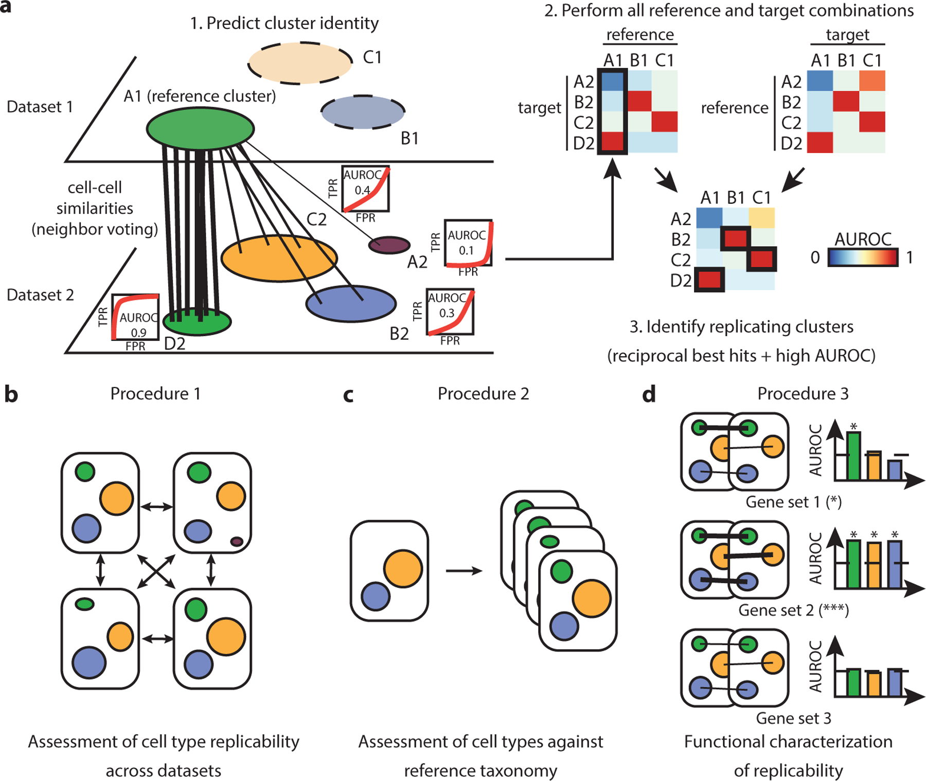
a Schematic of MetaNeighbor. MetaNeighbor uses a cross-dataset neighbor voting framework to compute cell type similarities. Cells from a reference cell type (A1) vote for cells in a target dataset according to their similarity (Spearman correlation). Votes can be summarized at the cell type level as an Area Under the Receiver Operating Characteristic curve (AUROC), reflecting the similarity of the reference and target cell types. Formally, the AUROC is computed for each pair of cluster by setting up the following classification problem: “can cells from the reference cluster (A1) predict which cells belong to the target cluster (e.g., D2)?”, where target cells are ranked according to their average similarity to A1 cells, cells from D2 are treated as positives, and all other cells from the target dataset are treated as negatives. An AUROC of 1 indicates perfect performance (all D2 cells ranked at the top). This procedure is repeated for all possible reference and target combinations: replicating cell types are identified as reciprocal top hits with high average AUROC. For example, D2 was A1’s top hit, reciprocally A1 was D2’s top hit, and the average AUROC of these hits exceeded 0.9. In AUROC graphs, TPR=True Positive Rate, FPR=False Positive Rate. b-d Schematic of the 3 MetaNeighbor procedures. Procedure 1 shows how to assess cell type replicability by considering all possible pairs of reference and target datasets: highly replicating cell types are identified as recurrent reciprocal top hits across datasets. Procedure 2 shows how to pre-train MetaNeighbor on large reference compendia, enabling rapid identification of reference cell types that are present in a given target dataset. Procedure 3 shows how to functionally characterize replicating cell types by identifying functional gene sets (such as Gene Ontology gene sets) that contribute most to replicability.

MetaNeighbor’s framework is flexible and can be adapted to multiple applications. In its supervised mode, it evaluates the replicability of cell types that are thought or known to be matching a priori. If, as is often the case, the cross-dataset cell type matching is unknown, MetaNeighbor also provides an unsupervised mode, which automatically identifies the strongest matching cell types and outputs the corresponding AUROCs. MetaNeighbor can also be used for the functional characterization of replicating cell types, identifying pre-defined gene sets (e.g., from the Gene Ontology or the HUGO Gene Nomenclature Committee) that contribute to cell type identity. Finally, the simplicity and scalability of the statistical framework facilitates the setup of computational control experiments.

To adapt to the emergence of large-scale datasets, which now routinely contain 100,000 cells or more, we improved MetaNeighbor’s implementation to quickly and interactively assess replicability for data compendia containing a high number of cells and independent experiments⁴. Aside from pure speed improvements, we added the possibility to compare a dataset to a pre-trained MetaNeighbor model, which allows the rapid evaluation of newly annotated data against comprehensive consortium data.

Applications of the method

In the original publication, we validated MetaNeighbor’s ability to characterize rare and transcriptionally subtle cell types¹⁵. Across 3 early transcriptomic neuron taxonomies, MetaNeighbor identified 11 strongly replicating interneuron subtypes, along with novel robust marker genes¹⁵. A similar analysis was performed across 7 datasets from the Brain Initiative Cell Census Network (BICCN), sampling from the mouse primary motor cortex using a variety of laboratories, technologies and clustering pipelines⁴. From the BICCN datasets, MetaNeighbor estimated that a majority (60/113) of the newly defined cell types were replicable and that these cell types were robustly identified across both sequencing technologies and clustering pipelines.

To further probe the basis of neuronal cell type identity, MetaNeighbor’s functional characterization identified gene families contributing to interneuron identity¹⁶, as well as conserved and divergent gene families across mouse, human and marmoset^6,17. Applied to a hand-picked selection of cardinal interneurons, MetaNeighbor showed that identity of these cell types could be characterized by gene families related to synaptic communication, which could be further subdivided into 6 broad categories (cell-adhesion molecules, transmitter-modulator receptors, ion channels, signaling proteins, neuropeptides and vesicular release components, transcription factors)¹⁶. Independently, MetaNeighbor was used to highlight conserved expression patterns between mouse and human neurons, showing that replicable cell types shared the same characteristic gene families in the two species¹⁷. These results were confirmed and extended in a cross-species analysis from the BICCN, where a MetaNeighbor analysis showed that the expression of genes relevant to neuron physiology (cadherins, ion channels, glutamate transporters) was preferentially conserved across human and marmoset compared to mouse⁶.

In the future, we believe that MetaNeighbor’s scalability will be further exploited to make accessible large consortium data (by querying pre-trained models) and meta-analyses (by enabling the comparison of large dataset compendia).

Overview of the Protocol

We present 3 procedures that use MetaNeighbor to quantify and characterize cell type replicability. In Procedure 1, we use unsupervised MetaNeighbor to identify replicable cell types across 4 pancreas datasets (Fig. 1b). In Procedure 2, we show how to assess newly annotated cell types against a large reference taxonomy by pre-training a MetaNeighbor model (Fig. 1c). Finally, in Procedure 3, we use supervised MetaNeighbor to investigate the molecular basis of cell type identity by finding functional gene sets that contribute highly to cell type replicability (Fig. 1d). All code blocks can be run in R command line, Rstudio, RMarkdown notebooks or a jupyter notebook with an R kernel.

To illustrate the procedures, we have chosen two data compendia that sample widely across laboratories and technologies. The pancreas compendium is commonly used in dataset integration assessments, samples from 4 different single-cell protocols, resulting in composition variability (e.g., rare epsilon cells are not detected in all datasets). The BICCN compendium is unique with respect to the size of the data (around half a million cells from 9 independent datasets targeting the same brain region), complexity of taxonomy (over a hundred cell types) and wide array of technologies used (single-cell transcriptomics, single-nuclei transcriptomics, single-nuclei methylation and single-nuclei chromatin accessibility).

Comparison with other methods

MetaNeighbor is related to four families of techniques: integrative methods designed to merge multiple datasets, methods for cell type annotation, metrics evaluating the quality of dataset integration, and metrics evaluating clustering robustness.

Integrative methods combine multiple datasets to improve cell type characterization. Mathematically, the rationale of these methods is to find a joint space that maximally preserves shared biological variation and removes all other variation. Popular methods include MNN⁸, Seurat^9,18, LIGER¹⁰, Harmony¹¹, Scanorama¹², and Conos¹³, which have been extensively reviewed^19,20 and benchmarked^21,22. The similarity with MetaNeighbor is the idea that batch effects are effectively attenuated by identifying mutual nearest neighbors. However, the aim is different: in integrative methods, mutual nearest neighbors are used to maximally correct and align datasets, while MetaNeighbor evaluates the similarity of nearest neighbors to quantify the amount of replicable signal. Methods for cell type annotation²³ (annotation of unlabeled cells by comparison with an annotated reference dataset), such as scmap²⁴ or Seurat⁹, are based on the same rationale of nearest neighbors. Again, the key difference with MetaNeighbor is the intent and interpretability: annotation methods output cell type labels, while MetaNeighbor outputs a statistic that lets the user evaluate how much replicable signal there is to begin with, providing complementary information about the expected robustness of these methods.

To evaluate dataset proximity, integration methods use metrics that quantify how successful the integration was. Popular metrics^21,22 include batch mixing metrics, such as kBET²⁵ and LISI¹¹, and cell type conservation metrics, such as ASW and ARI. Batch mixing metrics test whether datasets are well-mixed in the joint dataset space, which is seen as effective attenuation of technical variation. Cell type conservation metrics test whether biological variation is conserved, for example ASW tests whether cell types are well separated in the joint space, ARI checks that cell types obtained by clustering the integrated data are consistent with annotations from the independent data. However, these metrics are used to assess the performance of dataset integration, rather than evaluating the amount of replicable signal. Furthermore, in cases where datasets have limited biological overlap, these mixing metrics can be difficult to interpret, particularly if they are seen as scores that methods try to optimize. By always keeping datasets and annotations independent, MetaNeighbor’s focus is on rapidly identifying where data structure agrees but also differs, i.e. when cell types do not align across datasets or clustering pipelines.

In its design, MetaNeighbor is closest to methods for the validation of sample clustering, where the reproducibility of cluster structure across independent datasets is interpreted as “biological significance”²⁶, and which has been used to evaluate the reproducibility of cancer subtyping from microarray data^26,27. MetaNeighbor extends this framework to single cell genomics data and enables direct interpretation of gene sets whose co-expression drives replicability. Consensus clustering methods, such as SC3²⁸ or scrattch.hicat²⁹, are based on a similar idea, but the focus is on the quantification of robustness to clustering parameters or methods, while MetaNeighbor’s focus is on cross-dataset replicability, which includes variability due to clustering methods, but also lab-specific or conditional variability.

Experimental design

MetaNeighbor’s aim is to accurately estimate cell type replicability by preserving dataset independence. Consequently, we recommend using raw data and, if possible, cell type labels obtained by clustering each dataset independently (such as annotations from the original publication, if external data are used), which will help evaluate the robustness of cell types to the clustering procedure. If MetaNeighbor is run on data or labels that have been obtained through an integrative clustering technique, the user must be aware that dataset independence has been broken. Practically speaking, the integrative approach has a fitting step that will make datasets artificially similar, leading to optimistic replicability estimations. Similarly, even if datasets are truly independent, but MetaNeighbor is run in its unsupervised mode, replicability estimations will be slightly inflated, because the framework will automatically match the closest cell types.

Another problem that prevents accurate replicability estimation is the confounding of technical and biological variation, in the most extreme case when each cell type has been sequenced in a different batch. MetaNeighbor works best when batches are approximately balanced in terms of cell type composition, but can be adapted to confounded experimental designs. For example, MetaNeighbor has been adapted to an extreme case of confounding by replacing cross-dataset validation with simple cross-validation¹⁶. Results remain interpretable biologically but must be interpreted with greater care.

Thanks to its scalability, MetaNeighbor can be used to implement carefully designed control experiments. While we chose to output AUROCs because of its interpretability, its exact understanding depends on dataset composition and varies with cell type rarity and subtlety of transcriptomic differences between cell types. We proposed several control experiments that are simple to implement and help pinpoint how much signal can be expected to be extracted from the datasets under investigation¹⁵.

Expertise needed to implement the protocol

All three procedures are based on running R functions and require familiarity with the RStudio integrated development environment (IDE) or the R command line.

Limitations

Classification problems, and AUROCs in particular, are known to be affected by class imbalance (cell type composition in our case). Overall, MetaNeighbor is robust to such imbalances, but we found that scores can be distorted when class imbalance becomes extreme, in particular when there is no overlap between datasets. Benchmarking and evaluation to explore variability in performance is of continued interest and likely increasing importance if sampled data becomes more targeted. MetaNeighbor can be used to compare transcriptomic and epigenomic data, such as chromatin accessibility and methylation assays, but, in our experience, results are harder to interpret, in particular because there is no consensus on how to map genome-wide measurements with transcriptomic-wide measurements (see “Multi-modal analyses” in the “Anticipated Results” section). For very large datasets, MetaNeighbor can be memory intensive: when comparing several hundred thousand cells, we recommend using compute units or clusters that have a high memory capacity (>50–100Gb).

Materials

Equipment

Hardware

• A personal computer with internet connection and at least 8GB of RAM, ideally 16GB of RAM for Procedure 3.

Software

• RStudio (https://rstudio.com/products/rstudio/download/), Jupyter (https://jupyter.org/install) or R command line with R version 3.6 or higher.

• Key R package: the MetaNeighbor library, available on Github (https://github.com/gillislab/MetaNeighbor/) and Bioconductor version 3.12 or higher (https://doi.org/10.18129/B9.bioc.MetaNeighbor).

• Other R packages: scRNAseq, tidyverse, org.Hs.eg.db and UpSetR, available from Bioconductor (https://www.bioconductor.org/install/) and CRAN (https://cran.rstudio.com/).

Datasets

All procedures are based on published and publicly available datasets:

• Human pancreas datasets, accessed through the R/Bioconductor scRNAseq package (https://doi.org/doi:10.18129/B9.bioc.scRNAseq), which makes available a collection of publicly available single-cell transcriptomics datasets.

• The mouse primary visual cortex dataset, accessed through the scRNAseq package.

• The Brain Initiative Cell Census Network (BICCN) dataset for the mouse primary motor cortex. The full dataset is available on the NeMO archive (https://assets.nemoarchive.org/dat-ch1nqb7), the relevant subset of the dataset is directly available on Figshare (https://doi.org/doi:10.6084/m9.figshare.13020569.v2).

Equipment setup

This section walks through the installation process of MetaNeighbor and the packages used in the protocol. The installation process takes 1–20 minutes, depending on the number of dependencies already available. All code blocks can be run in R command line, Rstudio, RMarkdown notebooks or a jupyter notebook with an R kernel. CRITICAL: the installation process may create conflicts in the notebook environment. We recommend running the installation process in a separate R shell or to restart the Rstudio R environment after the installation has completed and before starting one of the procedures.

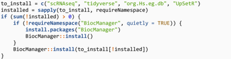
Start by installing the latest MetaNeighbor package from the Gillis lab GitHub page.

Note that the latest stable version of MetaNeighbor is also available through Bioconductor by running BiocManager::install(“MetaNeighbor”). We recommend using the latest development version from Github, as some of the functionalities illustrated in this protocol require Bioconductor version 3.12 or higher to work (only available with R version 4.0 or higher).

?TROUBLESHOOTING

Next, install the following packages, which are not necessary to run MetaNeighbor itself, but are needed to run the protocol.

CRITICAL STEP: Don’t forget to restart the R session at this stage. ?TROUBLESHOOTING

Procedure 1: assessment of cell type replicability with unsupervised MetaNeighbor

CRITICAL Procedure 1 demonstrates how to compute and visualize cell type replicability across 4 human pancreas datasets, detailing how to download and reformat the datasets with the SingleCellExperiment package and how to compute and interpret MetaNeighbor AUROCs.

Creation of a merged SingleCellExperiment dataset (1–2 minutes)

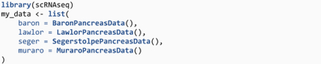
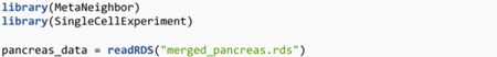
• 1We consider 4 pancreatic datasets along with their independent annotation (from the original publications). MetaNeighbor expects a gene-by-cell matrix encapsulated in a SummarizedExperiment format. We recommend the SingleCellExperiment (SCE) package, an extension of the SummarizedExperiment class designed to efficiently store large single-cell datasets, as it is able to handle sparse matrix formats. Load the pancreas datasets using the scRNAseq package, which provide annotated datasets that are already in the SingleCellExperiment format:

  

  Note that Seurat objects can easily be converted into SingleCellExperiment objects by using the as.SingleCellExperiment function for Seurat v3 objects and Convert(from = seurat_object, to = “sce”) for Seurat v2 objects.

• 2MetaNeighbor’s mergeSCE function can be used to merge multiple SingleCellExperiment objects. Importantly, the output object will be restricted to genes, metadata columns and assays that are common to all datasets. Before using mergeSCE, make sure that gene and metadata information aligns across datasets.

  Start by checking if gene information aligns (stored in the rownames slot of the SCE object):

  

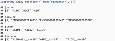
  Two datasets (Baron, Segerstolpe) use gene symbols, one dataset (Muraro) combines symbols with chromosome information (to avoid duplicate gene names) and the last dataset (Lawlor) uses Ensembl identifiers. Here we will convert all gene names to unique gene symbols. Start by converting gene names in the Muraro dataset by using the symbols stored in the rowData slot of the SCE object, and remove all duplicated gene symbols:

  

  Next, convert Ensembl IDs to gene symbols in the Lawlor dataset, removing all IDs with no match and all duplicated symbols:

  

• 3We now turn our attention to metadata, which are stored in the colData slot of the SCE objects. Here, make sure that the column that contains cell type information is labeled identically in all datasets:

  

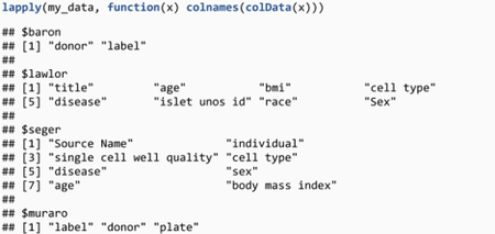
  Two datasets have the cell type information in the “cell type” column, the other two in the “label” column. Add a “cell type” column in the latter two datasets:

  

• 4Last, check that count matrices, stored in the assays slot, have identical names:

  

  

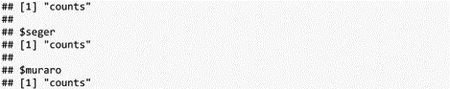
  The count matrices are all stored in an assay named “counts”, no change is needed here.

• 5Now that gene, cell type and count matrix information is aligned across datasets, create a merged dataset using mergeSCE, which takes a list of SCE objects as an input and outputs a single SCE object:

  

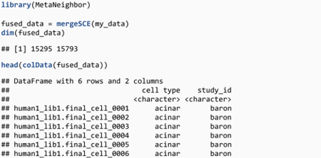
  The new dataset contains 15,295 common genes, 15,793 cells and two metadata columns: a concatenated “cell type” column, and “study_id”, a column created by mergeSCE containing the name of the original studies (corresponding to the names provided in the “my_data” list).

• 6To obtain a cursory overview of cell type composition by study, cross-tabulate cell type annotations by study IDs:

  

  

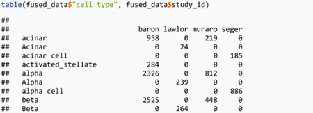
  Most cell types are present in all datasets, so we expect MetaNeighbor to find multiple high confidence matches across datasets. There are slight typographic differences in cell type annotations (e.g., ductal/Ductal), but we recommend keeping the author annotations at this stage. The only procedure that requires identical annotations across datasets is Procedure 3, where we perform functional characterization of replicating cell types.

• 7To avoid having to recreate the merged object, save the R object to a file using R’s RDS format:

  

  PAUSE POINT: the remaining sections of the procedure can be run at a later time in a new R session.

Hierarchical cell type replicability analysis (1 minute)

• 8Start by loading the MetaNeighbor (analysis) and the SingleCellExperiment (data handling) libraries, as well as the previously created pancreas dataset:

  

• 9To perform neighbor voting and identify replicating cell types, MetaNeighbor builds a cell-cell similarity network, which we defined as the Spearman correlation over a user-defined set of genes. We found that we obtained best results by picking genes that are highly variable across datasets, which can be done using the variableGenes function. Select highly variable genes for the pancreas datasets:

  

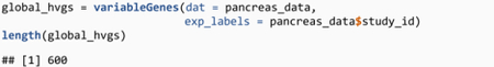
  The function returns a list of 600 genes that were detected as highly variable in each of the 4 datasets. In our experience, we obtained best performance for gene sets ranging from 200 to 1,000 variable genes. In general, using a larger number of datasets selects robustly varying genes, enabling high performance with a smaller number of genes. However, if variableGenes returns a gene set that is too small (in particular when you are comparing a large number of datasets), the number of genes can be increased by setting the “min_recurrence” parameter. For example, by setting “min_recurrence=2”, we keep all genes that are highly variable in at least 2 out of the 4 datasets. Additionally, genes are sorted by relevance in the latest version of MetaNeighbor, so it is always possible to select a smaller number of genes. For example, global_hvgs[1:500] selects the top 500 highly variable genes that are recurrent across all 4 datasets. This option can be used to validate that performance is robust over gene sets of increasing size.

  CRITICAL STEP: Variable genes are MetaNeighbor’s only parameter and must be selected with care (see Anticipated Results).

  ?TROUBLESHOOTING

• 10The merged dataset and a set of biologically meaningful genes is all that is needed to run MetaNeighbor and obtain cell type similarities. Because the dataset is large (> 10k cells), run the fast implementation of MetaNeighbor (“fast_version=TRUE”):

  

  MetaNeighborUS returns a cell-type-by-cell-type matrix containing cell type similarities. Cell type similarities are defined as an Area Under the ROC curve (AUROC), which range between 0 and 1, where 0 indicates low similarity and 1 high similarity. Note that the “fast_version=TRUE” parameter uses a slightly simplified version of MetaNeighbor that is significantly faster and more memory efficient. It should always be used on large datasets (> 10k cells), but can also be run on smaller datasets and yields equivalent results to the original MetaNeighbor algorithm.

  ?TROUBLESHOOTING

• 11For ease of interpretation, visualize AUROCs as a heatmap, where rows and columns are cell types from all the datasets:

  

  In the heatmap (Fig. 2), the color of each square indicates the proximity of a pair of cell types, ranging from blue (low similarity) to red (high similarity). For example, “baron|gamma” (2nd row) is highly similar to “seger|gamma” (3rd column from the right) but very different from “muraro|duct” (middle column). To group similar cell types together, plotHeatmap applies hierarchical clustering on the AUROC matrix. On the heatmap, we see two large red blocks that indicate hierarchical structure in the data, with endocrine cell types clustering together (e.g., alpha, beta, gamma) and non-endocrine cells on the other side (e.g., amacrine, ductal, endothelial). Note that each red block is composed of smaller red blocks, indicating that cell types can be matched at an even higher resolution. The presence of off-diagonal patterns (e.g., “lawlor|Gamma/PP”, “lawlor|Delta”) suggests the presence of doublets or contamination, but the heatmap is dominated by the clear presence of red blocks, which is a strong indicator of replicability.

  In the latest version of MetaNeighbor, we increased the flexibility of heatmaps. plotHeatmap internally relies on gplots::heatmap.2: you can pass any valid heatmap.2 parameter to plotHeatmap, for example the “ColSideColors” parameter can be used to annotate the columns of the heatmap (one color by dataset). Alternatively, the MetaNeighbor::ggPlotHeatmap function returns a customizable ggplot2 object.

  ?TROUBLESHOOTING

• 12To identify pairs of replicable cell types, run the following function:

  

  topHits relies on a simple heuristic: a pair of cell types is replicable if they are reciprocal top hits (they preferentially vote for each other) and the AUROC exceeds a given threshold value (in our experience, 0.9 is a good heuristic value). We find a long list of replicable endocrine cell types (e.g., epsilon, alpha and beta cells) and non-endocrine cell types (e.g. mast, endothelial or acinar cells) (Table 1). This list provides strong evidence that these cell types are robust, as they are identified across all datasets with high AUROC.

• 13In the case where there is a clear structure in the data (endocrine vs non-endocrine here), we can refine AUROCs by splitting the data. AUROCs have a simple interpretation: an AUROC of 0.6 indicates that cells from a given cell type are ranked in front of 60% of other target cells. However, this interpretation is outgroup dependent: because endocrine cells represent ~65% of cells, even an unrelated pair of non-endocrine cell types will have an AUROC > 0.65, because non-endocrine cells will always be ranked in front of endocrine cells.

  By starting with the full datasets, we uncovered the global structure in the data (endocrine vs non-endocrine). However, to evaluate replicability of endocrine cell types and reduce dataset composition effects, we can make the assessment more stringent by restricting the outgroup to close cell types, i.e. by keeping only endocrine subtypes. Split cell types in two by using the splitClusters function and retain only endocrine cell types:

  

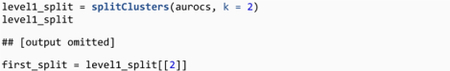
  By outputting “level1_split”, we found that the cell types were nicely split between non-endocrine and endocrine, and that endocrine cell types were in the second element of the list. Note that splitClusters applies a simple hierarchical clustering algorithm to separate cell types, however cell types can be selected manually in more complex scenarios.

• 14Repeat the MetaNeighbor analysis on endocrine cells only. First, subset the data to the endocrine cell types that were previously stored in “first_split”:

  

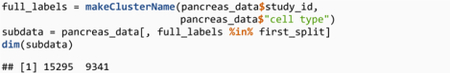
  The new dataset contains the 9341 putative endocrine cells.

• 15To focus on variability that is specific to endocrine cells, re-pick highly variable genes:

  

  ?TROUBLESHOOTING

• 16Finally, recompute cell type similarities and visualize AUROCs:

  

  

  The resulting heatmap (Fig. 3a) illustrates an example of a strong set of replicating cell types: when the assessment becomes more stringent (restriction to closely related cell types), the similarity of replicating cell types remains strong (AUROC~1 for alpha, beta, gamma, delta and epsilon cells) while the cross-cell-type similarity decreases (shift from red to blue, e.g. similarity of alpha and beta cell types has shifted from orange/red in the global heatmap to dark blue in the endocrine heatmap) by virtue of zooming in on a subpart of the dataset.

  ?TROUBLESHOOTING

• 17We can continue to zoom in as long as there are at least two cell types per dataset. Repeat steps 13–16 to split the endocrine cell types:

  

  Here we remove the alpha and beta cells (representing close to 85% of endocrine cells) and validate that, even when restricting to neighboring cell types, there is still a clear distinction between delta, gamma and epsilon cells (AUROC ~ 1, Fig. 3b).

  ?TROUBLESHOOTING

Figure 2. Cell types from 4 pancreas datasets cluster according to their biological similarity.

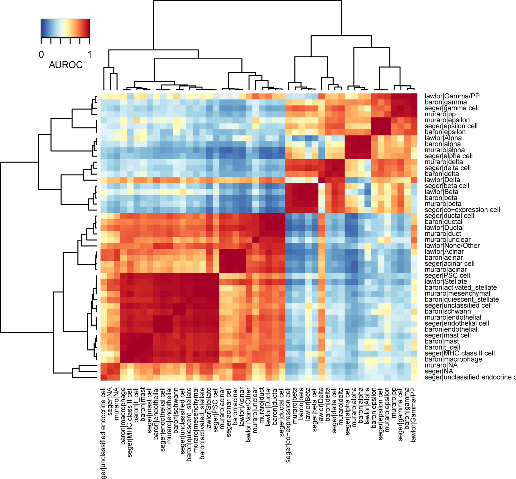
Heatmap based on MetaNeighbor AUROCs. Red indicates high similarity, blue indicates low similarity. By applying hierarchical clustering, replicating cell types group together (dark red squares), biologically related cell types (e.g. endocrine cell types, such as alpha, beta, gamma cells) form secondary groups (large light red squares).

Table 1. Reciprocal top hits with high AUROC identify replicating cell types.

Pairs of cell types that meet the following criteria: reciprocal top hits (the cell types preferentially vote for each other in the cross-dataset voting framework) or average AUROC > 0.9 (average taken by switching reference and target dataset).

Study_ID|Celltype_1	Study_ID|Celltype_2	Mean_AUROC	Match_type
seger|epsilon cell	muraro|epsilon	1.00	Reciprocal_top_hit
seger|epsilon cell	baron|epsilon	1.00	Above_0.9
baron|mast	seger|mast cell	1.00	Reciprocal_top_hit
seger|endothelial cell	muraro|endothelial	1.00	Reciprocal_top_hit
lawlor|Stellate	seger|PSC cell	1.00	Reciprocal_top_hit
baron|macrophage	seger|MHC class II cell	1.00	Reciprocal_top_hit
muraro|endothelial	baron|endothelial	1.00	Above_0.9
lawlor|Stellate	baron|activated_stellate	1.00	Above_0.9
baron|acinar	lawlor|Acinar	1.00	Reciprocal_top_hit
seger|PSC cell	muraro|mesenchymal	1.00	Above_0.9
baron|alpha	lawlor|Alpha	1.00	Reciprocal_top_hit
lawlor|Acinar	seger|acinar cell	1.00	Above_0.9
baron|schwann	seger|unclassified cell	1.00	Reciprocal_top_hit
seger|acinar cell	muraro|acinar	0.99	Above_0.9
lawlor|Beta	seger|beta cell	0.99	Reciprocal_top_hit
baron|ductal	seger|ductal cell	0.99	Reciprocal_top_hit
lawlor|Beta	baron|beta	0.99	Above_0.9
baron|ductal	lawlor|Ductal	0.99	Above_0.9
seger|MHC class II cell	baron|t_cell	0.99	Above_0.9
baron|gamma	lawlor|Gamma/PP	0.99	Reciprocal_top_hit
lawlor|Beta	muraro|beta	0.98	Above_0.9
seger|ductal cell	muraro|duct	0.98	Above_0.9
lawlor|Alpha	muraro|alpha	0.98	Above_0.9
seger|PSC cell	baron|quiescent_stellate	0.98	Above_0.9
lawlor|Gamma/PP	seger|gamma cell	0.98	Above_0.9
seger|delta cell	muraro|delta	0.98	Reciprocal_top_hit
lawlor|Gamma/PP	muraro|pp	0.98	Above_0.9
muraro|alpha	seger|alpha cell	0.98	Above_0.9
muraro|delta	baron|delta	0.96	Above_0.9
baron|beta	seger|co-expression cell	0.95	Above_0.9
seger|ductal cell	muraro|unclear	0.93	Above_0.9
baron|delta	lawlor|Delta	0.92	Above_0.9
baron|ductal	lawlor|None/Other	0.91	Above_0.9

Figure 3. Restricting the 4 pancreas datasets to endocrine subtypes allows for a more stringent replicability assessment.

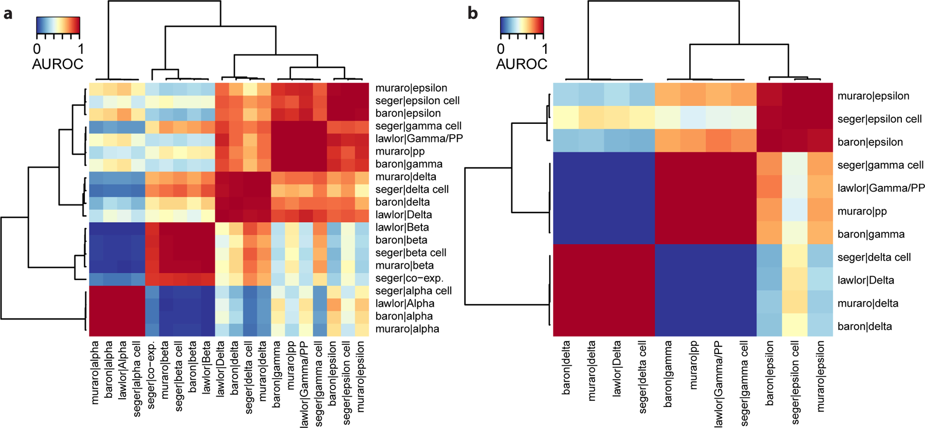
a Heatmap based on MetaNeighbor AUROCs applied to endocrine cell types, where cell types are grouped by applying hierarchical clustering. Red squares represent replicating cell types (alpha, beta, gamma, delta and epsilon cells). b AUROCs can be refined as long as there are two cell types per dataset. Heatmap based on MetaNeighbor AUROCs applied to gamma, delta and epsilon cells, where cell types are grouped by applying hierarchical clustering. Red squares represent replicating cell types (gamma, delta and epsilon cells).

Stringent assessment of replicability with one-vs-best AUROCs (1 minute)

CRITICAL In the previous section, we created progressively more stringent replicability assessments by selecting more and more specific subsets of related cell types. As an alternative, we provide the “one_vs_best” parameter, which offers similar results without having to restrict the dataset manually. In this scoring mode, MetaNeighbor will automatically identify the two closest matching cell types in each target dataset and compute an AUROC based on the voting result for cells from the closest match against cells from the second closest match. Essentially, we are asking how easily a cell type can be distinguished from its closest neighbor.

• 18To obtain one-vs-best AUROCs, run the same command as before with two additional parameters: “one_vs_best = TRUE” and “symmetric_output = FALSE”:

  

  

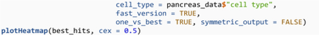
  The interpretation of the heatmap is slightly different compared to one-vs-all AUROCs (Fig. 4). First, since we only compare the two closest cell types, most cell type combinations are not tested (NAs, shown in gray on the heatmap). Second, by setting “symmetric_output=FALSE”, we broke the symmetry of the heatmap: reference cell types are shown as columns and target cell types are shown as rows. Since each cell type is only tested against two cell types in each target dataset (closest and second closest match), we have 8 values per column (2 per dataset).

  This representation helps to rapidly identify a cell type’s closest hits as well as its closest outgroup. For example, ductal cells (2nd red square from the top right) strongly match with each other (one-vs-best AUROC>0.8) and acinar cells are their closest outgroup (blue segments in the same column). The non-symmetric view makes it clear when best hits are not reciprocal. For example, mast cells (first two columns) heavily vote for “lawlor|Stellate” and “muraro|mesenchymal”, but this vote is not reciprocal. This pattern indicates that the mast cell type is missing in the Lawlor and Muraro datasets: because mast cells have no natural match in these datasets, they vote for the next closest cell type (stellate cells). The lack of reciprocity in voting is an important tool to detect imbalances in dataset composition.

  ?TROUBLESHOOTING

• 19When using one-vs-best AUROCs, we recommend extracting replicating cell types as meta-clusters. Cell types are part of the same meta-cluster if they are reciprocal best hits. Note that if cell type A is the reciprocal best hit of B and C, all three cell types are part of the same meta-cluster, even if B and C are not reciprocal best hits. To further filter for strongly replicating cell types, we specify an AUROC threshold (in our experience, 0.7 is a strong one-vs-best AUROC threshold). To extract meta-clusters and summarize the strength of each meta-cluster, run the following functions:

  

  The scoreMetaClusters function provides a good summary of meta-clusters, ordering cell types by the number of datasets in which they replicate, then by average AUROC. We find 12 cell types that have strong support across at least 2 datasets, with 7 cell types replicating across all 4 datasets. 8 cell types are tagged as “outlier”, indicating they had no strong match in any other dataset. These cell types usually contain doublets, low quality cells or contaminated cell types. To rapidly visualize the number of robust cell types, the replicability structure can be summarized as an Upset plot with the plotUpset function (Fig. 5a).

  

  To further investigate the robustness of meta-clusters, they can be visualized as heatmaps (called “cell-type badges”) with the plotMetaClusters function. Because the function generates one heatmap per meta-cluster, save the output to a PDF file to facilitate investigation:

  

  Each badge shows an AUROC heatmap restricted to one specific meta-cluster. These badges help diagnose cases where AUROCs are lower in a specific reference or target dataset. For example, the “muraro|duct” cell type has systematically lower AUROCs, suggesting the presence of contaminating cells in another cell type (probably in the “muraro|unclear” cell type) (Fig. 5b).

• 20The last visualization is an alternative representation of the AUROC heatmap as a graph, which is particularly useful for large datasets. In this graph, top votes (AUROC > 0.5) are shown in gray, while outgroup votes (AUROC < 0.5) are shown in orange. To highlight close calls, we recommend keeping only strong outgroup votes, here with AUROC >= 0.3. To build and plot the cluster graph, run the following functions:

  

  We note that there are several orange edges, indicating that some cell types had two close matches (Fig. 5c). To investigate the origin of these close calls, we can focus on a cluster of interest (coi). Take a closer look at “baron|epsilon”, query its closest neighbors in the graph with extendClusterSet, then zoom in on its subgraph with subsetClusterGraph:

  

  In the “baron|epsilon” case, we find that the epsilon cell type is missing in the Lawlor dataset, so there is no natural match for the Baron epsilon cell type (Fig. 5d). In such cases, votes are frequently non-reciprocal and equally split between two unrelated cell types, here “Lawlor|Gamma/PP” and “Lawlor|Alpha”. In general, the cluster graph can be used to understand how meta-clusters are extracted, why some clusters are tagged as outliers and diagnose problems where the resolution of cell types differs across datasets.

Figure 4. 1-vs-best AUROCs automatically identify each cell type’s closest outgroup.

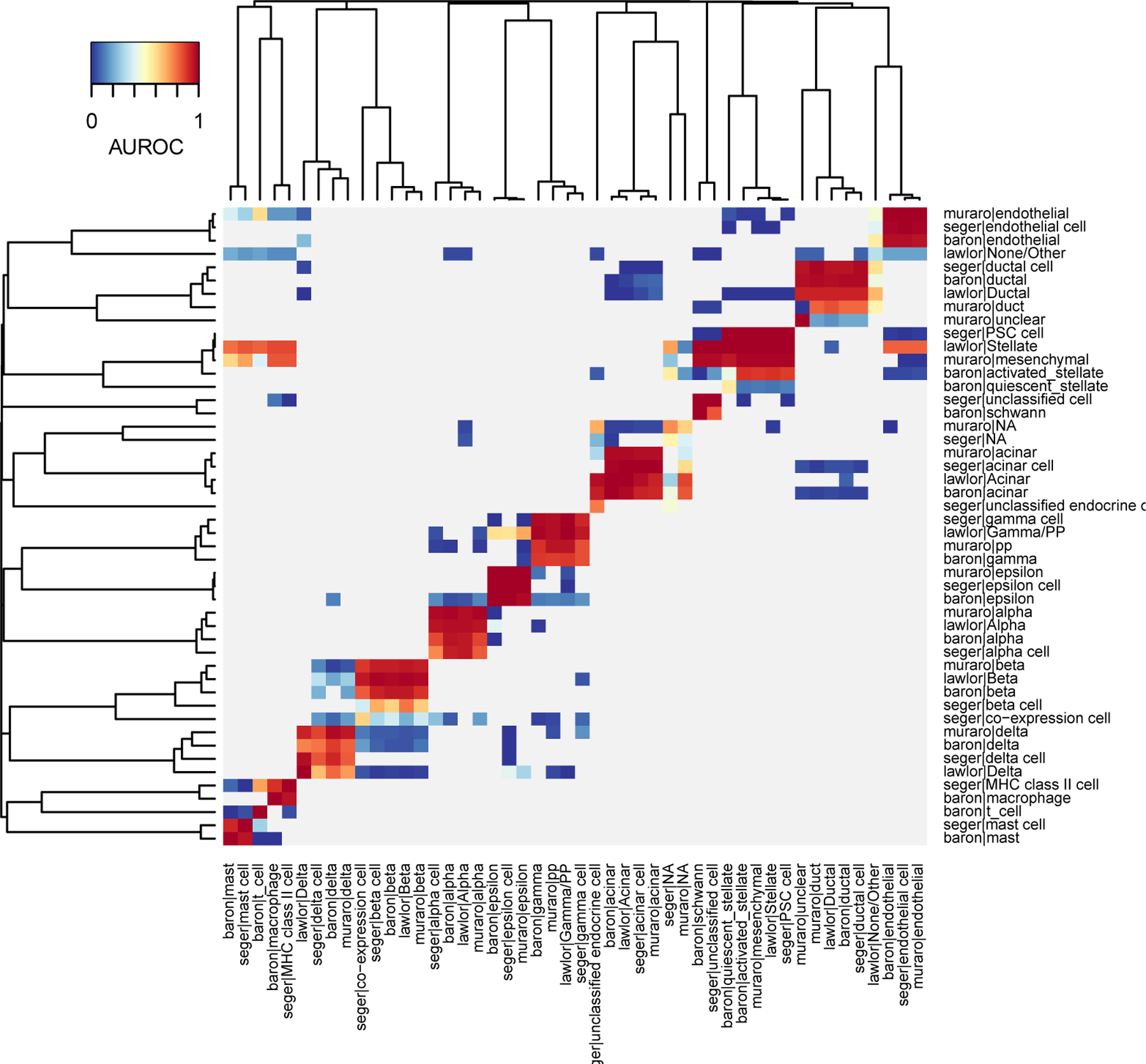
Heatmap based on MetaNeighbor 1-vs-best AUROCs, where cell types are grouped by applying hierarchical clustering. Reference cell types are shown as columns, target cell types are shown as rows. Red values indicate each reference cell type’s best hit, blue values the closest outgroup (one value per target dataset). All other cell type combinations are shown in gray.

Figure 5. Replicating cell types can be extracted as meta-clusters.

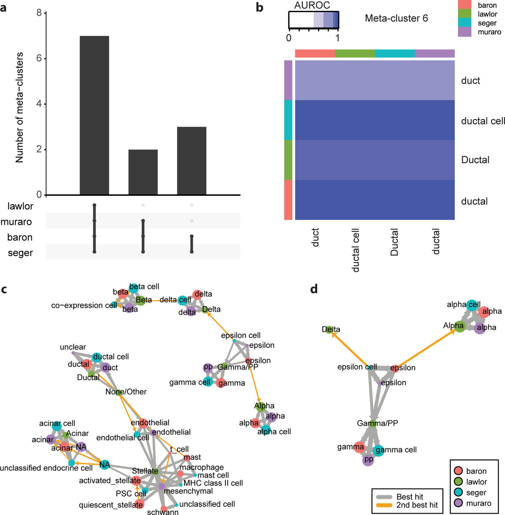
a The Upset plot breaks down cell-type replicability by dataset. Meta-clusters (groups of replicating cell types) are organized according to the datasets in which they replicate. For example, there are two cell types that replicate in the Baron, Muraro and Seger datasets, but are missing in the Lawlor dataset. b “Cell type badges” help identify datasets where cell type replicability is weaker. 1-vs-best AUROC heatmap for meta-cluster corresponding to ductal cells. The cell type is detected across all 4 datasets, but AUROCs are systematically weaker when testing in the Muraro dataset, indicating that the cell type is not as clearly defined in that dataset. c The cluster graph enables the rapid visualization of replicating cell types. Each node of the graph represents a cell type, colored by dataset of origin. Best hits (strong 1-vs-best AUROC) are shown by gray directed edges (oriented from reference cell type toward target cell type). Outgroups are shown by orange directed edges (reference toward target) for 1-vs-best AUROC > 0.3. Ideally replicating cell types form cliques (every pair of a cell type is connected, e.g., alpha cells). d Subsetting the cluster graph enables the investigation of close calls. Same representation as c, centered on the “epsilon” cell type from the Baron dataset, which had two close matches in the Lawlor dataset (“Alpha” and “Gamma/PP”), as the epsilon cell type is missing in the Lawlor dataset.

Procedure 2: Assessing cell type replicability against a pre-trained reference taxonomy

CRITICAL Procedure 2 demonstrates how to assess cell types of a newly annotated dataset against a reference cell type taxonomy. Pre-training a MetaNeighbor model provides a rigorous, fast and simple way to query a large reference dataset and obtain quantitative estimations of the replicability of newly annotated clusters. In Procedure 1, all datasets needed to be loaded simultaneously, which may be prohibitive when large datasets are involved. Pre-training a model enables to load large datasets only once, when the pre-trained model is generated. The pre-trained model only requires a small amount of memory, which makes it easy to share and query, particularly for large atlas taxonomies. In this procedure, we consider the cell type taxonomy established by the Brain Initiative Cell Census Network (BICCN) in the mouse primary motor cortex. The BICCN taxonomy was defined across a compendium of datasets sampling across multiple modalities (transcriptomics and epigenomics); it constitutes one of the richest neuronal resources currently available. When matching against a reference taxonomy, we assume that the reference is of higher resolution than the query dataset, i.e. the query dataset samples the same set or a subset of cells compared to the reference.

Pre-train a reference MetaNeighbor model (1–5 minutes)

• 1Start by loading an already merged SCE object containing the BICCN dataset. The full code for generating the dataset is available on Github³⁰, the dataset can be downloaded directly on FigShare³¹.

  

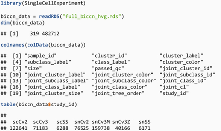
  The BICCN data contains 7 datasets totaling 482,712 cells. There are multiple sets of cell type labels depending on resolution (class, subclass, cluster) or type of labels (independent labels or labels defined from joint clustering). Note that, to reduce memory usage, we have already computed and restricted the dataset to a set of 319 highly variable genes.

• 2Create pre-trained models with the trainModel function, which has identical parameters as the MetaNeighborUS function used in Procedure 1. Here, we choose to focus on two sets of cell types: subclasses from the joint clustering (medium resolution, e.g., Vip interneurons, L2/3 IT excitatory neurons), and clusters from the joint clustering (high resolution, e.g., Chandelier cells). Create and store pre-trained models at the subclass level, then at the cluster level:

  

  

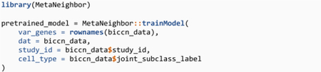
  For simplicity of use, we store the pretrained models to file using the write.table function.

  PAUSE POINT: The remainder of the procedure is independent and can be run in a new R session.

Compare annotations to pre-trained taxonomy (1 minute)

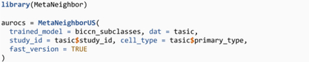
• 3Start by loading the query dataset (Tasic 2016, neurons from mouse primary visual cortex³⁶, available in the scRNAseq package) and the pre-trained subclass and cluster taxonomies:

  

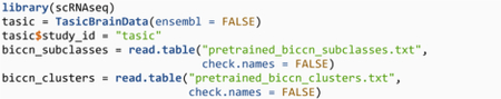
  We add a “study_id” column to the Tasic metadata, as this information will be needed later by MetaNeighbor. Note the “check.names = FALSE” argument when reading a pre-trained model, which is required to preserve the correct formatting of MetaNeighbor cell type names.

• 4To run MetaNeighbor, we use the MetaNeighborUS function but, compared to Procedure 1, we provide a pre-trained model instead of a set of highly variable genes (which are already contained in the pre-trained model). Start by checking if Tasic cell types are consistent with the BICCN subclass resolution:

  

  ?TROUBLESHOOTING

• 5Visualize AUROCs as a rectangular heatmap, with the reference taxonomy cell types as columns and query cell types as rows (Fig. 6a):

  

  As in Procedure 1, we start by looking for evidence of global structure in the dataset. Here we recognize 3 red blocks, which correspond to non-neurons (top left), inhibitory neurons (middle) and excitatory neurons (bottom right). The presence of sub-blocks inside the 3 global blocks suggest that cell types can be matched more finely. For example, inside the inhibitory block, we can recognize sub-blocks corresponding to CGE-derived interneurons (Vip, Sncg and Lamp5 in the BICCN taxonomy) and MGE-derived interneurons (Pvalb and Sst in the BICCN taxonomy).

• 6Refine AUROCs by focusing on inhibitory neurons using the splitTrainClusters and splitTestClusters utility functions to select the relevant cell types:

  

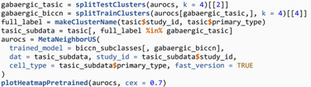
  The heatmap (Fig. 6b) suggests that there is a broad agreement at the subclass level between the BICCN MOp taxonomy and the Tasic 2016 dataset. For example, the Ndnf subtypes, Igtp and Smad3 cell types from the Tasic dataset match with the BICCN Lamp5 subclass.

  ?TROUBLESHOOTING

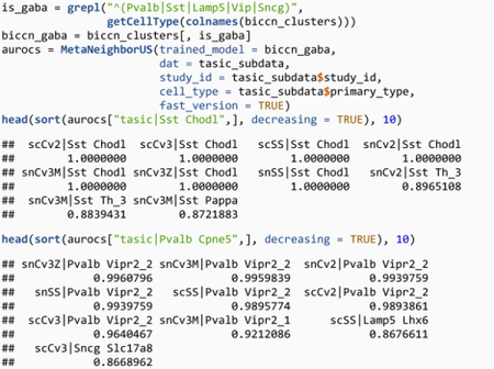
• 7The previous heatmaps suggest that all Tasic cell types can be matched with one BICCN subclass. We now go one step further and ask whether inhibitory cell types correspond to one of the BICCN clusters. Compute and visualize cell type similarity:

  

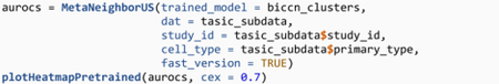
  Here the heatmap is difficult to interpret due to the large number of BICCN cell types (Fig. 7a). Instead, investigate the top hits for each query cell type directly:

  

  

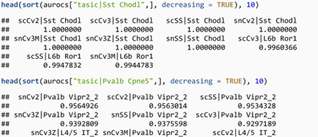
  We note two properties of matching against a pre-trained reference. First, replicable cell types have a clear top match in each of the reference dataset. Sst Chodl (long-projecting interneurons) match to similarly named clusters in the BICCN with an AUROC > 0.9999, Pvalb Cpne5 (Chandelier cells) match with the Pvalb Vipr2_2 cluster with AUROC > 0.93. Second, we have to be beware of false positives. For example, Sst Chodl secondarily matches with the L6b Ror1 cell types with AUROC > 0.98, an excitatory cell type only distantly related with long-projecting interneurons. When we use the pre-trained model, we only compute AUROCs with the BICCN data as the reference data, so we cannot identify reciprocal hits. If we had been able to use “Tasic|Sst Chodl” as the reference cluster, its votes would have gone heavily in favor of the BICCN’s Sst Chodl, making L6b Ror1 a low AUROC match on average. Because of the low dimensionality of gene expression space, we expect false positive hits to occur just by chance (e.g., cell types reusing similar pathways) when a cell type is missing in the query dataset. Here L6b Ror1 (an excitatory type) had no natural match with the Tasic inhibitory cell types and voted for its closest match, long-projecting interneurons.

  There are three alternatives to separate true hits from false positive hits. First, if a cell type is highly replicable, it will have a clear top matching cluster in the reference dataset. Second, if the query dataset is known to be a particular subset of the reference dataset (e.g., inhibitory neurons, as is the case here), we recommend restricting the reference taxonomy to that subset. Third, if the first two solutions don’t yield clear results or cannot be performed, it is possible to go back to reciprocal testing by using the full BICCN dataset instead of the pre-trained reference.

  ?TROUBLESHOOTING

• 8We illustrate the first solution in the case of Chandelier cells (Fig. 7b). Visualize the strength of the best hits by running the following:

  

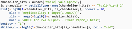
  To illustrate AUROC differences, we chose a logarithmic scaling to reflect that AUROC values do not scale linearly: when AUROCs are close to 1, a difference of 0.05 is substantial. Here, the best matching BICCN cluster (“Pvalb Vipr2_2”) is orders of magnitude better than other clusters, suggesting very strong replicability.

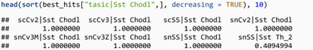
• 9The second solution to avoid false positive hits is to subset the reference to cell types that reflect the composition of the query datasets. Since we are looking at inhibitory neurons, restrict the BICCN taxonomy to inhibitory cell types, whose names all start with “Pvalb”, “Sst”, “Lamp5”, “Vip” or “Sncg”:

  

  Again, we note that there is a significant gap between the best hit and the secondary hit, but now secondary hits are closely related cell types (Sst subtype for Sst Chodl, secondary Chandelier cell type Pvalb Vipr2_1 for Pvalb Cpne5).

  ?TROUBLESHOOTING

• 10To obtain a more stringent mapping between the query cell types and reference cell types, compute one-vs-best AUROC, which will automatically match the best hit against the best secondary hit:

  

  Now the hit structure is much sparser, which helps identify 1:1 and 1:n hits (Fig. 8). The heatmap suggests that most Tasic cell types match with one or several BICCN clusters. Inspect the top hits for 3 cell types from the Tasic dataset:.

  

  

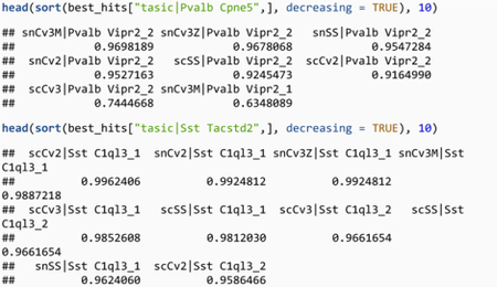
  Using this more stringent assessment, we confirm that Sst Chodl strongly replicates inside the BICCN (one-vs-best AUROC ~ 1, best secondary hit = 0.41), and observe the same for Pvalb Cpne5 (one-vs-best AUROC > 0.74, best secondary hit = 0.63), while for example Sst Tacstd2 corresponds to multiple BICCN subtypes (including Sst C1ql3_1, Sst C1ql3_2, AUROC > 0.95).

Figure 6. Assessment of cell type annotations from the mouse primary visual cortex against reference neuron taxonomy from the primary motor cortex (medium resolution).

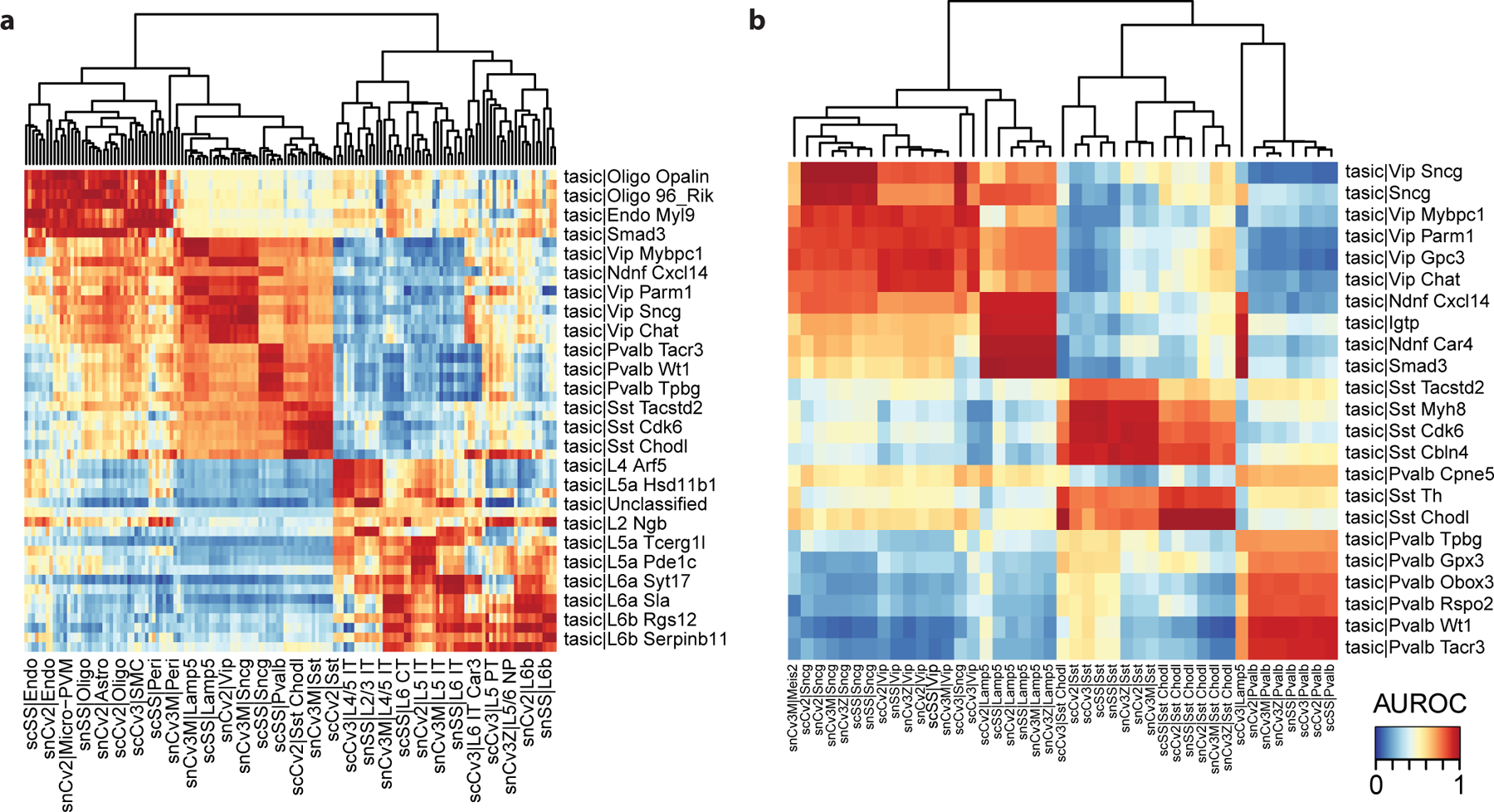
a Heatmap based on MetaNeighbor AUROCs. Reference cell types are shown as columns, query cell types as rows. Reference cell types are grouped by hierarchical clustering, query cell types according to the strongest matching reference cell type. b Assessment of inhibitory cell types from the mouse primary visual cortex against reference inhibitory cell types (medium resolution). Same representation as a. Red rectangles indicate groups of related cell types: Sncg, Vip, Lamp5, Sst and Pvalb inhibitory neurons.

Figure 7. Assessment of inhibitory cell types from the mouse primary visual cortex against reference inhibitory cell types (high resolution).

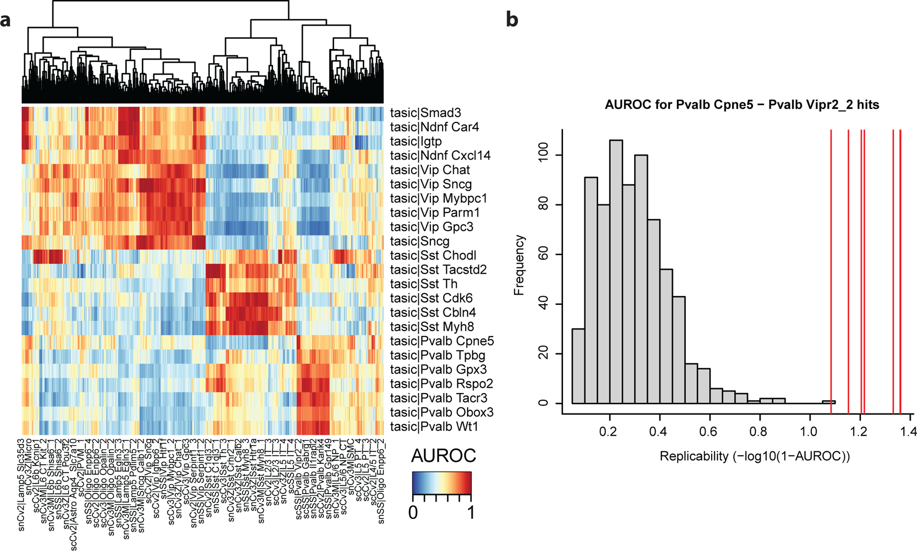
a Heatmap based on MetaNeighbor AUROCs. Reference cell types are shown as columns, query cell types as rows. Global red rectangles indicate good replicability structure, suggesting replicability for Sncg, Vip, Lamp5, Sst and Pvalb inhibitory subtypes. b Distribution of AUROC scores for the “Pvalb Cpne5” cell type from the primary visual cortex (query cell type) against all reference cell types. Best hits (against the “Pvalb Vipr2_2) are shown by red lines, all other hits are shown as a gray background distribution. Replicating cell types have substantially higher AUROC scores than background cell types.

Figure 8. 1-vs-best AUROCs enable rapid identification of 1:1 hits and 1:n hits.

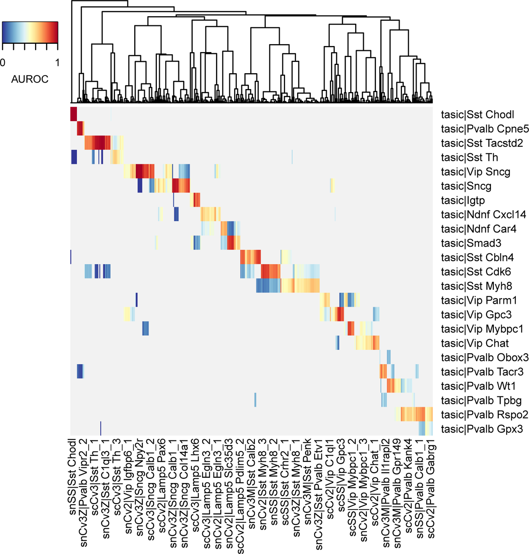
Heatmap is based on MetaNeighbor 1-vs-best AUROCs. Reference cell types are shown as columns, query cell types as rows. In this representation, the best hits are shown in red, the outgroup hit is shown in blue, all other values are gray.

Procedure 3: Functional characterization of replicating clusters

CRITICAL Procedure 3 demonstrates how to characterize functional gene sets contributing to cell type identity. Once replicating cell types have been identified with unsupervised MetaNeighbor (as in Procedures 1 and 2), supervised MetaNeighbor enables the functional interpretation of the biology contributing to each cell type’s identity. In this procedure, we will focus on the characterization of inhibitory neuron subclasses from the mouse primary cortex as provided by the BICCN. The BICCN has shown that subclasses are strongly replicable across datasets and provided marker genes that are specific to each subclass. MetaNeighbor can be used to further quantify which pathways contribute to the subclasses’ unique biological properties.

Creation of biologically relevant gene sets (1 minute)

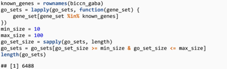
• 1To compute the functional characterization of clusters, we first need an ensemble of gene sets sampling relevant biological pathways. In this procedure we will consider the Gene Ontology (GO) annotations for mouse. The scripts used to build up-to-date gene sets can be found on Github³⁰ and gene sets can be downloaded directly on FigShare³¹. Start by loading the GO sets:

  

  Gene sets are stored as a named list, where each element of the list corresponds to a gene set and contains a vector of gene symbols.

• 2Load the dataset containing inhibitory neurons from the BICCN. The scripts used to build the dataset can be found on Github³⁰ and the dataset can be downloaded on FigShare³¹.

  

• 3Next, restrict the gene sets to genes that are present in the dataset. Then, filter gene sets to keep gene sets of meaningful size: large enough to learn expression profiles (> 10), small enough to represent specific biological functions or processes (< 100):

  

Functional characterization with supervised MetaNeighbor (30–90 minutes)

• 4Once the gene set list is ready, run the supervised MetaNeighbor function. Its inputs are similar to MetaNeighborUS, but it assumes that cell types have already been matched across datasets (i.e., they have identical names). Here we use joint BICCN subclasses, for which names have been normalized across datasets (“Pvalb”, “Sst”, “Sst Chodl”, “Vip”, “Lamp5”, “Sncg”). Note that, because we are testing close to 6,500 gene sets, this step is expected to take a long time for large datasets. We recommend using this function inside a script and always saving results to a file as soon as computations are done by using the write.table function.

  

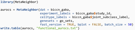
  Later, results can be retrieved with the read.table function:

  

  ?TROUBLESHOOTING

• 5Use the plotBPlot function on the first 100 gene sets to visualize how replicability depends on gene sets (Fig. 9).

  

  In this representation, large segments represent average gene set performance and short segments represent the performance of individual gene sets. We note that most gene sets contribute moderately to replicability (AUROC ~ 0.7), numerous gene sets have a performance close to random (AUROC ~ 0.5 – 0.6) and some gene sets have exceedingly high performance (AUROC > 0.8).

• 6To focus on gene sets that contribute highly to cell type specificity, create a summary table containing, for each gene set, cell type specific AUROCs, average AUROCs across cell types and gene set size:

  

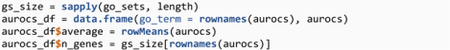
  Then, order gene sets by average AUROC and look at the top scoring gene sets (Table 2).

  

  Without surprise, replicability is mainly driven by gene sets related to neuronal functions that are immediately relevant to the physiology of inhibitory neurons, such as “glutamate receptor signaling pathway”, “regulation of synaptic transmission, glutamatergic”, or “chemical synaptic transmission, postsynaptic”. Note that most of the top scoring gene sets have a large number of genes, as larger sets of genes make it easier to learn generalizable expression profiles.

  To obtain even more specific biological functions, further filter for gene sets that have fewer than 20 genes (Table 3).

  

  Again, the top scoring gene sets are dominated by biological functions immediately relevant to inhibitory neuron physiology, such as “ionotropic glutamate receptor signaling pathway”, “positive regulation of synaptic transmission, GABAergic”, or “GABA-A receptor complex”.

• 7To understand how individual genes contribute to gene set performance, use the plotDotPlot function, which shows the expression of all genes in a gene set of interest, averaged over all datasets (Fig. 10):

  

  

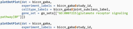
  High scoring gene sets are characterized by the differential usage of genes from a given gene set. For example, when looking at the GABA-A receptor complex composition, Lamp5 preferentially uses the Gabrb2 and Gabrg3 receptors, Pvalb the Gabra1 receptor, and Sst Chodl the Gabra2, Gabrb1 and Gabrg1 receptors (Fig. 10b).

Figure 9. A small fraction of functional gene sets contributes highly to cell type replicability.

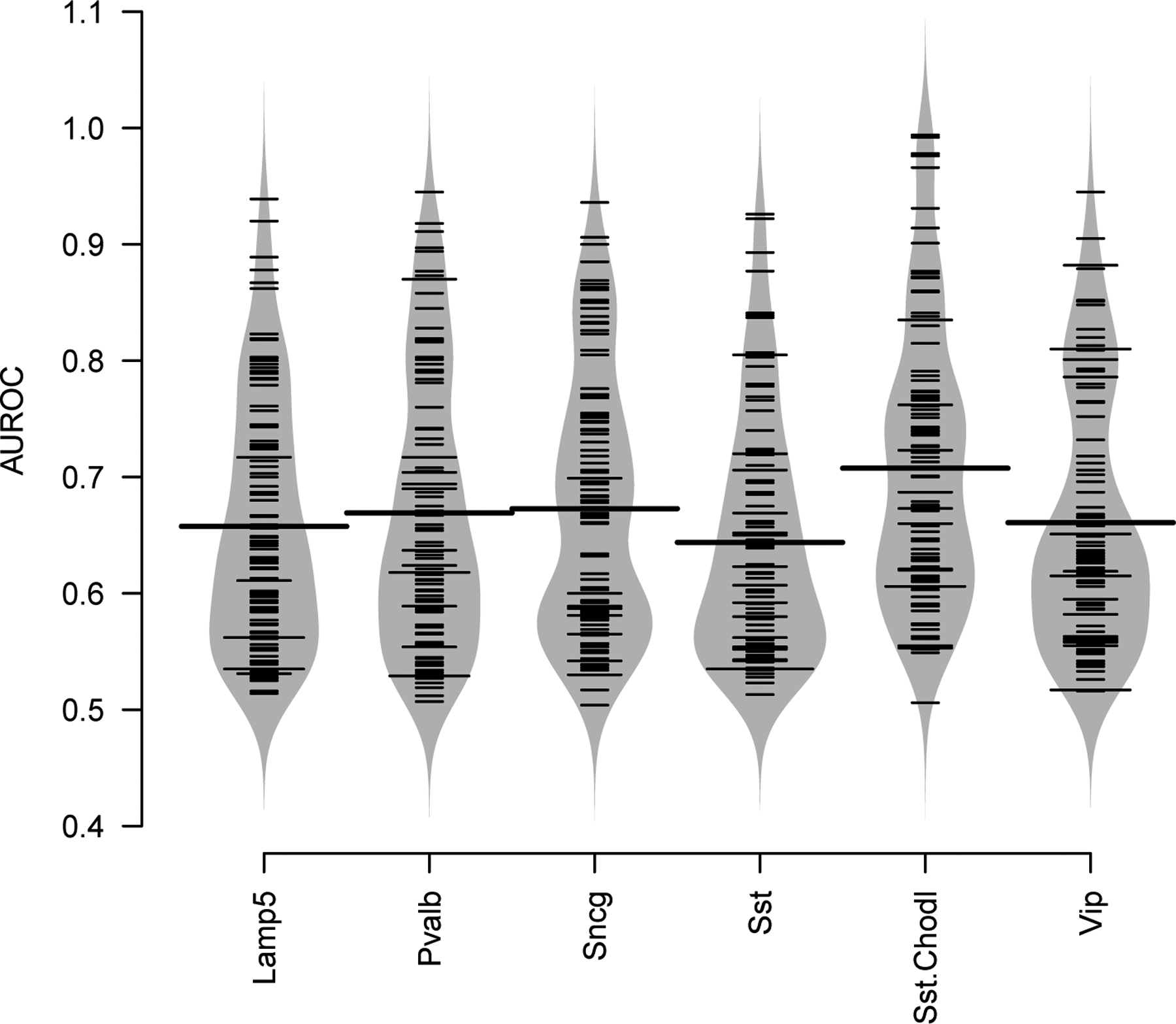
For each cell type, large ticks represent the average AUROC across gene sets. Each smaller tick represents an individual gene set, the envelope is a violin-plot style approximation of the distribution of performance across gene sets.

Table 2. Top 10 gene sets (with fewer than 100 genes) contributing to cell type replicability.

The “go_term” column shows the identifier, name, and sub-ontology (BP=Biological Process, CC=Cellular Component) of the investigated gene set. Columns “Lamp5” to “Vip” show the replicability (average AUROC over cross-dataset-validation folds) for each cell type and gene set combination. The “average” column takes the average across cell types, “n_genes” shows the number of genes in the gene set.

go_term	Lamp5	Pvalb	Sncg	Sst	Sst.Chodl	Vip	average	n_genes
GO:0007215|glutamate receptor signaling pathway|BP	0.97	0.98	0.97	0.98	1.00	0.99	0.98	92
GO:0051966|regulation of synaptic transmission, glutamatergic|BP	0.96	0.97	0.98	0.96	0.99	0.97	0.97	75
GO:0060076|excitatory synapse|CC	0.96	0.97	0.99	0.96	0.99	0.96	0.97	75
GO:0033555|multicellular organismal response to stress|BP	0.95	0.98	0.98	0.95	1.00	0.98	0.97	98
GO:0098839|postsynaptic density membrane|CC	0.92	0.97	0.98	0.98	0.98	0.97	0.97	93
GO:0099565|chemical synaptic transmission, postsynaptic|BP	0.97	0.98	0.97	0.95	0.99	0.96	0.97	91
GO:0008306|associative learning|BP	0.97	0.98	0.96	0.96	0.99	0.95	0.97	100
GO:0099601|regulation of neurotransmitter receptor activity|BP	0.96	0.98	0.96	0.95	0.99	0.98	0.97	61
GO:0060079|excitatory postsynaptic potential|BP	0.97	0.98	0.97	0.95	0.99	0.95	0.97	83
GO:0010771|negative regulation of cell morphogenesis involved in differentiation|BP	0.98	0.98	0.97	0.96	0.99	0.92	0.97	98

Table 3. Top 10 gene sets (with fewer than 20 genes) contributing to cell type replicability.

Same format as Table 2.

go_term	Lamp5	Pvalb	Sncg	Sst	Sst.Chodl	Vip	average	n_genes
GO:0004970|ionotropic glutamate receptor activity|MF	0.90	0.92	0.91	0.96	0.97	0.92	0.93	19
GO:0035235|ionotropic glutamate receptor signaling pathway|BP	0.82	0.82	0.91	0.93	0.94	0.87	0.88	16
GO:0032230|positive regulation of synaptic transmission, GABAergic|BP	0.84	0.86	0.82	0.92	0.98	0.83	0.88	16
GO:0007216|G protein-coupled glutamate receptor signaling pathway|BP	0.89	0.85	0.76	0.92	0.95	0.84	0.87	16
GO:1905874|regulation of postsynaptic density organization|BP	0.83	0.86	0.87	0.90	0.92	0.83	0.87	19
GO:0099150|regulation of postsynaptic specialization assembly|BP	0.83	0.89	0.86	0.91	0.91	0.80	0.87	18
GO:0150052|regulation of postsynapse assembly|BP	0.83	0.89	0.86	0.91	0.91	0.80	0.87	18
GO:0021889|olfactory bulb interneuron differentiation|BP	0.81	0.91	0.82	0.88	0.89	0.86	0.86	15
GO:0070679|inositol 1,4,5 trisphosphate binding|MF	0.92	0.94	0.79	0.81	0.86	0.85	0.86	15
GO:1902711|GABA-A receptor complex|CC	0.82	0.87	0.87	0.80	0.99	0.80	0.86	19

Figure 10. Top scoring gene sets can be broken down into characteristic genes for each cell type.

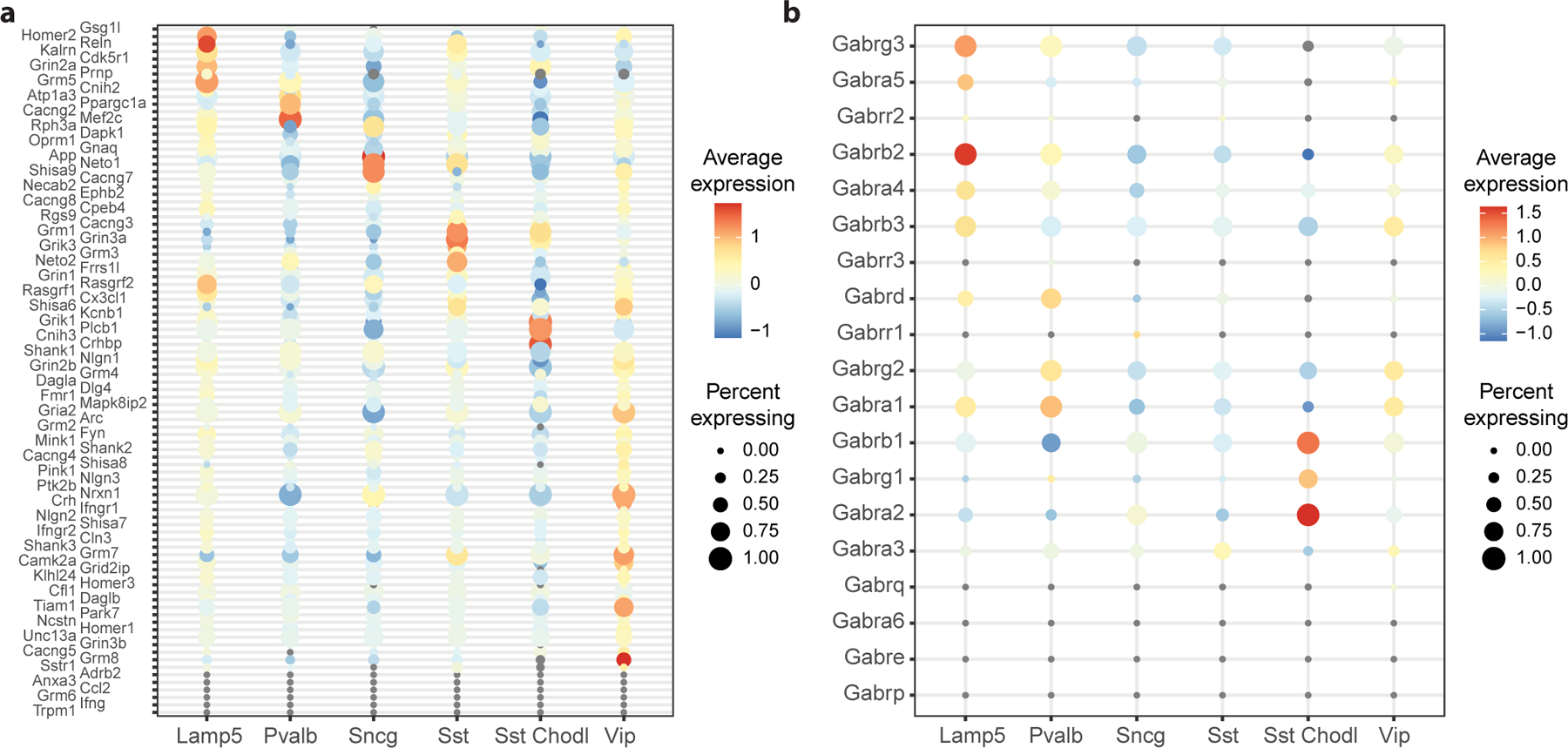
a Dot plot of genes from the “Glutamate receptor signalling pathway” Gene Ontology term, where cell types are shown on the x-axis and genes are shown on the y-axis. For each cell type, the dot size corresponds to the fraction of cells expressing a given gene, the color corresponds to the z-scored average expression level, averaged across datasets. b Same as a, for the “GABA-A receptor complex” Gene Ontology term.

Timing

The expected timing for the procedures is as follows:

• Procedures 1 and 2: 1 to 5 minutes each.

• Procedure 3: 30 to 90 minutes.

The first two procedures (assessment of cell type replicability) can be run interactively: once the data are loaded, every call to MetaNeighbor returns within seconds, which enables looking at the data in different ways, for example by zooming in on different parts of the dataset. In contrast, procedure 3 (functional characterization of replicability) is intended to be run as a script, allowing testing thousands of gene sets and analyzing results within a day.

Note that the exact timing depends on the hardware and software used, notably the amount of memory and the BLAS (Basic Linear Algebra Subprograms) library used. MetaNeighbor relies heavily on matrix operations, leading to large speed-ups when using the Intel MKL (Math Kernel Library) BLAS or openBLAS instead of R’s native BLAS library.

Troubleshooting

Troubleshooting guidance can be found in Table 4.

Table 4.

Troubleshooting table.

Step	Problem	Possible reason	Solution
Equipment Setup	Installation failed: package could not be downloaded.	Running command in the notebook fails because user input is expected.	Run command directly as R command line instead of notebook.
Procedure 1 - Step 9, 15, 17	variableGenes returns “Cholmod error ‘problem too large’”	Matrix is too large to be properly handled.	Downsample datasets with “downsampling_size” parameter or manually downsample datasets.
Procedure 1 - Step 10, 16, 17, 18 Procedure 2 - Step 4, 6, 7, 9, 10 Procedure 3 - Step 4	MetaNeighbor returns “Cholmod error ‘problem too large’”	One of the datasets is too large to be properly handled.	Use smaller gene sets, downsample largest dataset or run on batches of datasets, then combine AUROC matrices.
	MetaNeighbor returns “Error: cannot allocate vector of size XXX Gb”	Legacy MetaNeighbor was used on a large dataset (>10k cells)	Use “fast_version = TRUE”. If this does not solve the problem, see above.
	MetaNeighbor returns rows or columns that contain only NAs.	One dataset contains only one cell type.	This is expected behavior (no outgroup to compare against). Ignore NAs, use “symmetric_output=FALSE” or make sure to keep at least two cell types when subsetting datasets.
Procedure 1 - Step 11, 16, 17, 18	plotHeatmap returns “Error in M + t(M): non-conformable arrays”	plotHeatmap has been applied to non-square AUROC matrix, likely because MetaNeighbor was run on a pre-trained model.	Use plotHeatmapPretrained instead.
	In Rstudio, plotHeatmap causes “Error in plot.new() : figure margins too large”	The default Rstudio resolution is too low to correctly display heatmap.	In the code block options, increase “fig.width” and “fig.height” until resolved.

Anticipated results

Because MetaNeighbor is non-parametric, there is no fine-tuning to be done for any of the procedures presented here. Over time, we have identified two sources of potential error: bad highly variable gene selection and coding or formatting errors, which can be easily diagnosed by looking at AUROC heatmaps. As a rule of thumb, we expect AUROCs to correctly represent global relationships between cell types, contain replicable cell types (dark red squares or rectangles on heatmaps) and generalize across studies. In the examples below, we illustrate the most common places where these errors are found by presenting a side-by-side comparison of correct and problematic code.

Bad gene set selection

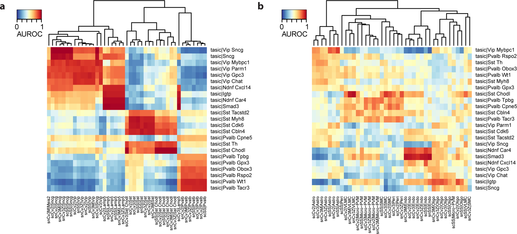
The most common problem is to forget to select a set of highly variable genes, which is expected to dampen the impact of technical variability on neighbor voting (Procedure 1, Steps 9–11). First, we present an example of a correct analysis, where we load the BICCN GABAergic neurons, select highly variable genes, and compute cluster similarities (see Procedure 1 for more details).

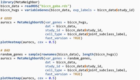
We recognize strong replicability structure, evidenced by the presence of dark red blocks (Fig. 11a). When we repeat the analysis with random genes, the replicability structure is still present, but we recognize two signatures of bad gene set selection: (a) AUROCs are low overall (shift to light red and orange), (b) within red blocks, there is a clear gradient structure (Fig. 11b). In our experience, there are 3 scenarios that lead to bad gene selection: errors in gene symbol conversion, errors when genes are stored as factors in R (that are implicitly converted to numerical values during indexing), and forgetting to select highly variable genes altogether.

Figure 11. Selection of a bad highly variable gene set leads to suboptimal performance and obscures biological signal.

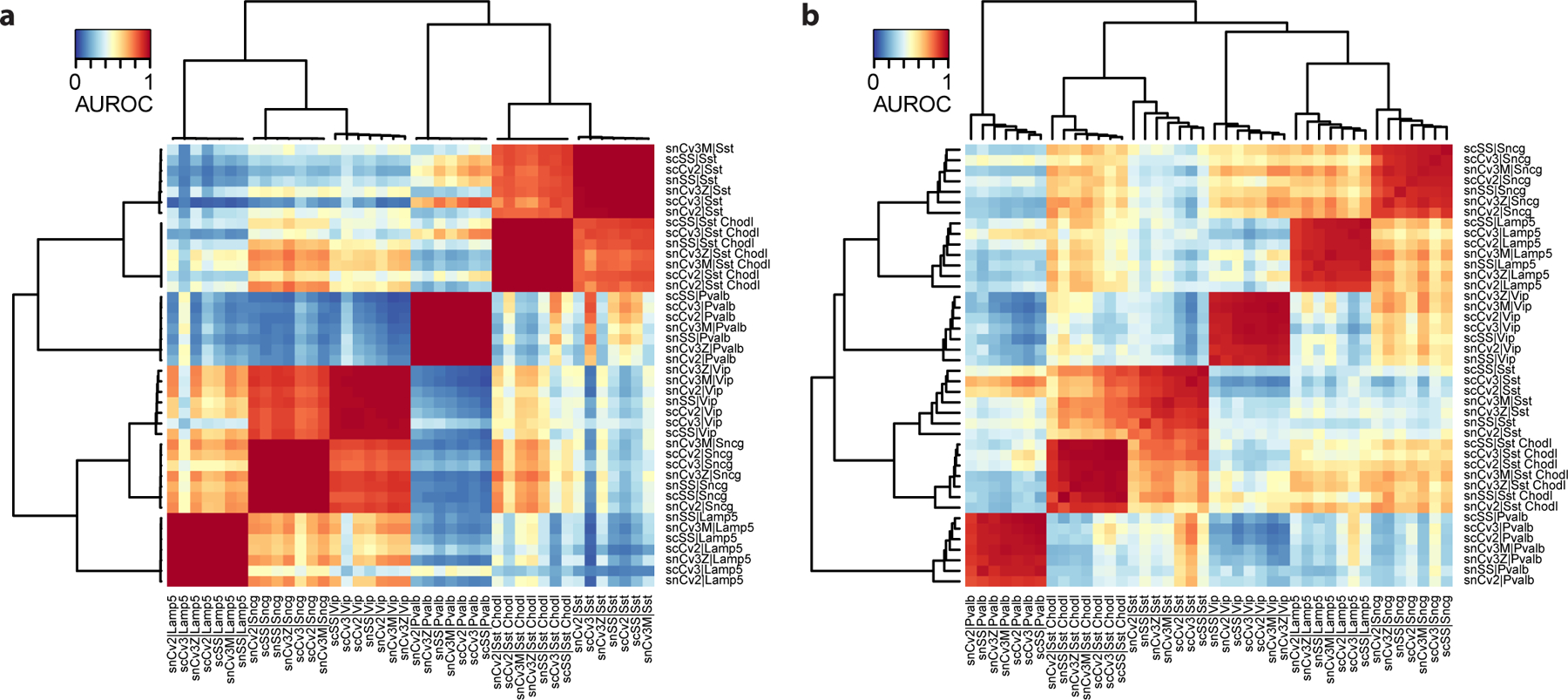
a Anticipated result: AUROC heatmap based on a set of highly variable genes selected by MetaNeighbor. The heatmap has clear replicating clusters (dark red squares) and known secondary biological relationships (e.g., similarity of CGE-derived interneurons Vip, Sncg and Lamp5). b Possible issue: AUROC heatmap based on a set of random genes (same number of genes as the correctly selected highly variable gene set in a). Replicability patterns become weaker: lower performance, gradients within replicating cell types, weaker secondary relationships.

No overlap between datasets

The second problem occurs when there is no overlap between datasets, which can be detected in Procedure 1 at Step 11 or Procedure 2 at Step 5–7. We illustrate this problem with the data from Procedure 2, where we expect all cell types from the Tasic dataset to be present in the pre-trained BICCN model. According to our expectations, all cell types have strong hits with BICCN clusters, and we see a hierarchical structure that is consistent with prior biological knowledge: lighter red blocks corresponding to Medial Ganglionic Eminence (MGE) and Caudal Ganglionic Eminence (CGE)-derived inhibitory neurons (Fig. 12a). We compare with the same block of code, where we “mistakenly” keep non-neurons from the BICCN taxonomy instead of inhibitory neurons. The lack of biological overlap can be deduced from 3 factors (Fig. 12b): (a) low AUROC values overall, (b) almost no strong hits (contrary to expectations), (c) lack of expected hierarchical structure (MGE and CGE derived inhibitory neurons).

Figure 12. Absence of biological overlap between datasets leads to almost random performance and lack of hierarchical cell type structure.

a Anticipated result: AUROC heatmap with inhibitory neuron cell types as query (rows) and inhibitory neuron cell types as reference (columns). b Possible issue: same as a, but with non-neuronal cell types as reference (columns). The heatmap lacks clear replicating clusters (dark red rectangles) and known secondary biological relationships (e.g., similarity of CGE-derived interneurons Vip, Sncg on the query side).

Pretrained MetaNeighbor: bad name formatting

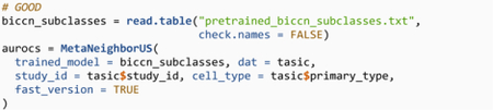
The third problem we have encountered is a mistake that occurs when loading a pre-trained model in Step 3 of Procedure 2 and forgetting to specify “check.names = FALSE”, which is essential to preserve correct formatting of cell type names. Below, we present an example of correct code based on data from Procedure 2. We obtain the expected replicability structure, with evidence of strong hits across all cell types (Fig. 13a, see Procedure 2 for further details and analyses). When we forget “check.names = FALSE”, MetaNeighbor is unable to correctly recognize dataset names and cell type names in the pre-trained model, the similarity computations become meaningless, leading to AUROC values that are essentially 0.5 (Fig. 13b). This problem is easy to diagnose and fix but can be very confusing when it occurs.

Figure 13. Disrupting formatting of cell type names in pre-trained models leads to random performance.

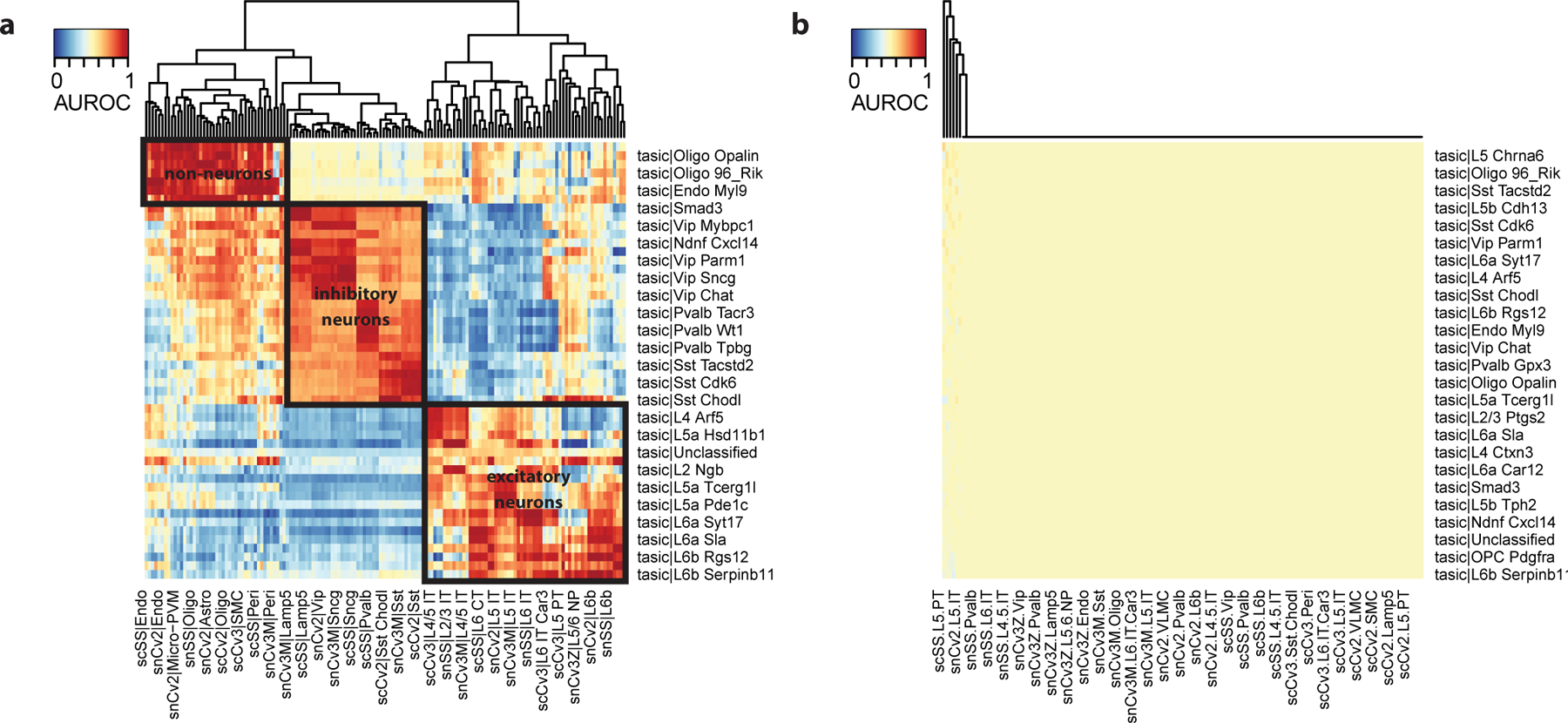
a Anticipated result: AUROC heatmap with cell types from primary visual cortex as query (rows) and cell types from primary motor cortex as reference (columns). The heatmap shows evidence of replicating cell types (dark red rectangles) and global structure (larger rectangles corresponding to non-neurons, excitatory neurons and inhibitory neurons). b Possible issue: same as a, but with incorrect formatting of reference cell types (due to an error while reading the pre-trained model), leading to completely random performance.

Impact of batch effects on cell type matching

The voting scheme used by MetaNeighbor is naturally robust to batch effects, as it relies on identifying nearest neighbors (which are approximately conserved in the presence of batch effects) rather than transcriptional similarity. Because cell type matching is determined based on reciprocal best hits (similar to BLAST), we expect MetaNeighbor results to be robust to a large range of batch effects and recommend using MetaNeighbor on unaligned datasets to obtain more accurate replicability values. As we show here, batch effects mainly affect the range of AUROC values, and should be considered when interpreting heatmaps (Procedure 1 Step 11, Procedure 2 Steps 5–7) and replicability strength (Procedure 1 Step 12, Procedure 2 Steps 8–10, Procedure 3 Steps 5–6).

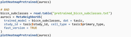
To illustrate the expected drop in AUROC with data quality, we simulated two types of batch effects in the pancreas compendium presented in the protocol: lower sensitivity and higher noise level. To simulate low sensitivity, we downsampled counts in endocrine cells of the Baron dataset and recorded the AUROCs of best hits in the 3 remaining datasets. AUROCs progressively declined, dropping below 0.9 around 250 UMIs per cell (Fig. 14a) and stabilizing around 0.8 for nearly-empty cells. Reciprocal top hits remained perfectly conserved, except for epsilon cells (the rarest cell type), where performance started to degrade around 100 UMIs per cell, which represents exceptionally low sensitivity (Fig. 14b). In the second batch effect simulation, we subset the Baron dataset to highly variable genes, then added gaussian noise with mean 0 and standard deviation f*average UMIs per cell, where f is the “fraction” of noise. We observed a similar pattern to downsampling experiments: AUROC progressively declined, dropping below 0.9 when the noise level reached around 10% of the average count value and progressively declined towards 0.8 (Fig. 14c). Again, reciprocal top hits were perfectly conserved, with a slight degradation for epsilon cells beyond 25% noise (Fig. 14d). In the original MetaNeighbor publication, we further showed that AUROCs are robust to cell type rarity and the presence of closely related cell types¹⁵.

Figure 14. MetaNeighbor results are robust to batch effects.

a Replicability (MetaNeighbor AUROC) of endocrine cell types in the Baron pancreas dataset after downsampling the number of Unique Molecular Identifiers (UMIs) per cell. “original” corresponds to the replicability in the original dataset, without downsampling (~ 5000 UMIs per cell). Line types represent the Highly Variable Gene (HVG) selection strategy: full lines indicate that the initial set of HVG (based on the full dataset) is conserved (“static”), dashed lines indicate that HVG are re-picked after downsampling (“variable”). b Stacked barplot showing the number of reciprocal top hits for each endocrine cell type after downsampling. The height of the bars indicates the number of datasets in which the cell type was found to replicate. c Replicability (MetaNeighbor AUROC) of endocrine cell types in the Baron pancreas dataset after the addition of noise to original counts. d Stacked barplot showing the number of reciprocal top hits for each endocrine cell type after the addition of noise. In all panels, statistics are averaged over 10 independent experiments and colors represent cell types.

In practice, we found that our AUROC guidelines (AUROC > 0.9, 1-vs-best AUROC > 0.7) held on datasets that spanned a wide range of quality and batch effects and should thus apply to most recently generated single cell datasets. For example, the BICCN datasets used in this protocol includes multiple types of batch effects, as it uses a large array of sequencing protocols⁴: differences in sensitivity (2,000 to 6,000 detected genes per cell), differences in cell type composition (L5 ET cells survive better in single nuclei protocols), systematic differences in expression profiles (PCR-amplification bias for Smart-Seq, higher expression of nuclear genes for nuclei protocols). However, if one of the datasets is known to be particularly noisy or low quality, the AUROCs for this dataset can be expected to be lower than the guidelines suggested in this manuscript, but we recommend using AUROC>0.8 and 1-vs-best AUROC>0.6 as a minimum.

Multi-modal analyses

MetaNeighbor can be applied to multi-modal analyses, but requires a gene by cell matrix for all modalities (all steps remain identical to the protocol presented here). In particular, modalities such as chromatin accessibility and methylation data require a mapping of peaks or reads to individual genes. This mapping is currently unclear, as many peaks are related to regulatory elements such as enhancers and cannot be attributed to individual genes, resulting in an important loss of signal. As discussed in the previous section, such losses can be seen as “batch effects” and result in lower AUROC values in some modalities (Procedure 1 Step 11–12, Procedure 2 Steps 5–10, Procedure 3 Steps 5–6).

We illustrate the results of a multi-modal analysis in the BICCN data for the mouse primary motor cortex⁴. The full multi-modal data include the 7 singe-cell and single-nucleus RNA-sequencing (scRNAseq) datasets presented in the protocol, a single-nucleus Assay for Transposase-Accessible Chromatin (ATAC) using sequencing dataset (“atac”) and a single-nucleus methylation dataset (“snmc”). The initial analysis reveals a difference in resolution between modalities: while there is a single cell type for L2/3 IT and L5 IT excitatory neurons in the scRNAseq datasets (at the “subclass” annotation level), there are multiple matching cell types in the ATAC and methylation annotations (Fig. 15a). The presence of clear red blocks (high AUROC with primary match, lower AUROC with secondary match) suggests that, for example, L23.a, L23.b and L23.c in ATACseq all correspond to the L2/3 IT type in scRNAseq. After merging L2/3 IT and L5 IT cell types under a single annotation, we find an excellent mapping between all modalities, resulting in a clear separation of individual cell types (Fig. 15b). Almost all extracted meta-clusters span all 9 datasets (Fig. 15c), with only a handful of cell types missing in one of the other modalities, such as L6b (missing in ATAC), non-neuron subclasses (unannotated in the methylation data) or L6 IT Car3 (missing in several datasets). All modalities share the same range of reciprocal top hits (Fig. 15d), suggesting that the same cell types have been successfully identified in all datasets. However, AUROC values are significantly lower in the ATAC data (Fig. 15e), suggesting that gene-level quantification only imperfectly captures the variability of the modality and a slightly more lenient AUROC threshold may be applied (e.g., AUROC>0.85). Note that MetaNeighbor can also be used for cross-species analyses⁶, and that similar considerations may apply. As more distant species are included in the analyses, expression signatures are expected to diverge, resulting in lower AUROC values overall.

Figure 15. MetaNeighbor finds replicable cell types in a multi-modal dataset of the mouse primary motor cortex.

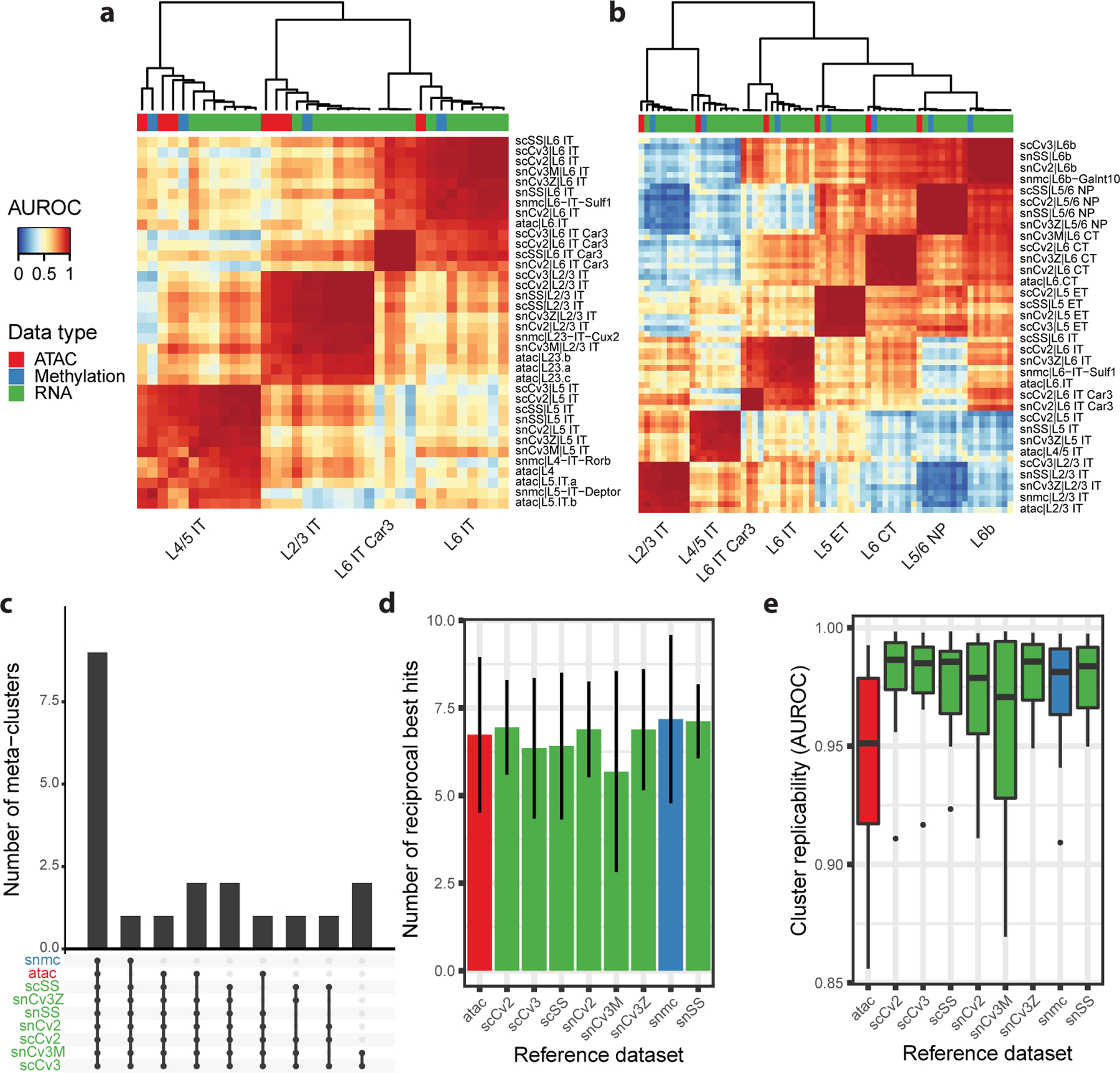
a Heatmap based on MetaNeighbor AUROCs for Intra-Telencephalic (IT) projecting cell types, where cell types are grouped by applying hierarchical clustering. Column annotation colors indicate the sequencing modality (expression, chromatin accessibility or methylation). b Heatmap based on MetaNeighbor AUROCs for excitatory cell types, where cell types are grouped by applying hierarchical clustering. Column annotation colors as in a. c Upset plot showing the number of cell types that replicate across given combinations of datasets (meta-clusters). For example, 9 cell types were found to replicate across all datasets. d Number of reciprocal best hits for each dataset in the primary motor cortex compendium. The height of each bar indicates the average number of hits across cell types, the line indicates the standard deviation. e Boxplot showing the strength of cluster replicability (MetaNeighbor AUROC) across cell types for each dataset in the primary motor cortex compendium. The lower and upper hinges of the boxplots represent the first and third quartile, the central line represents the median, the upper (resp. lower) whisker extends to the largest (resp. smallest) value within 1.5 IQR (Inter-Quartile Range) of the hinge. All points beyond 1.5 IQR are drawn individually.

Generalizable quantification of cell type similarities

In their computation, MetaNeighbor’s AUROCs are directly related to Spearman correlations. More precisely, all computations are based on average Spearman correlations between cells from two cell types, but include an additional prediction step that alleviates batch effects, while keeping an interpretability power that is comparable to correlations (where AUROC = 0 maps to correlation = −1, AUROC = 0.5 maps to correlation = 0, AUROC = 1 maps to correlation = 1).

To appreciate how the additional prediction step enables us to obtain “batch free correlations”, we compare MetaNeighbor’s output (Procedure 1 Step 11, Procedure 2 Steps 5–7) with a more naive similarity output, where we compute the Spearman correlation between cell type centroids (Fig. 16a). Centroid correlations display two desirable patterns: centroids cluster primarily by cell type (then by dataset) and global hierarchical structure is preserved (we can distinguish MGE-derived interneurons vs CGE-derived interneurons). However, batch effects are clearly visible throughout the heatmap. For example, within each cell type, Chromium-based datasets tend to cluster on one side, Smart-Seq-based datasets on the other side. In contrast, for an equivalent computation time, all the “good” patterns (cell types and hierarchical structure) are made pristinely clear with MetaNeighbor AUROCs (Fig. 16b), while technical substructure has been lost: technologies mix well within cell-types, homogenous cell groupings look uniform, and biological relationships between cell types are correctly displayed.

Figure 16. MetaNeighbor AUROCs offer a generalizable and batch-effect-free quantification of cell type similarity.

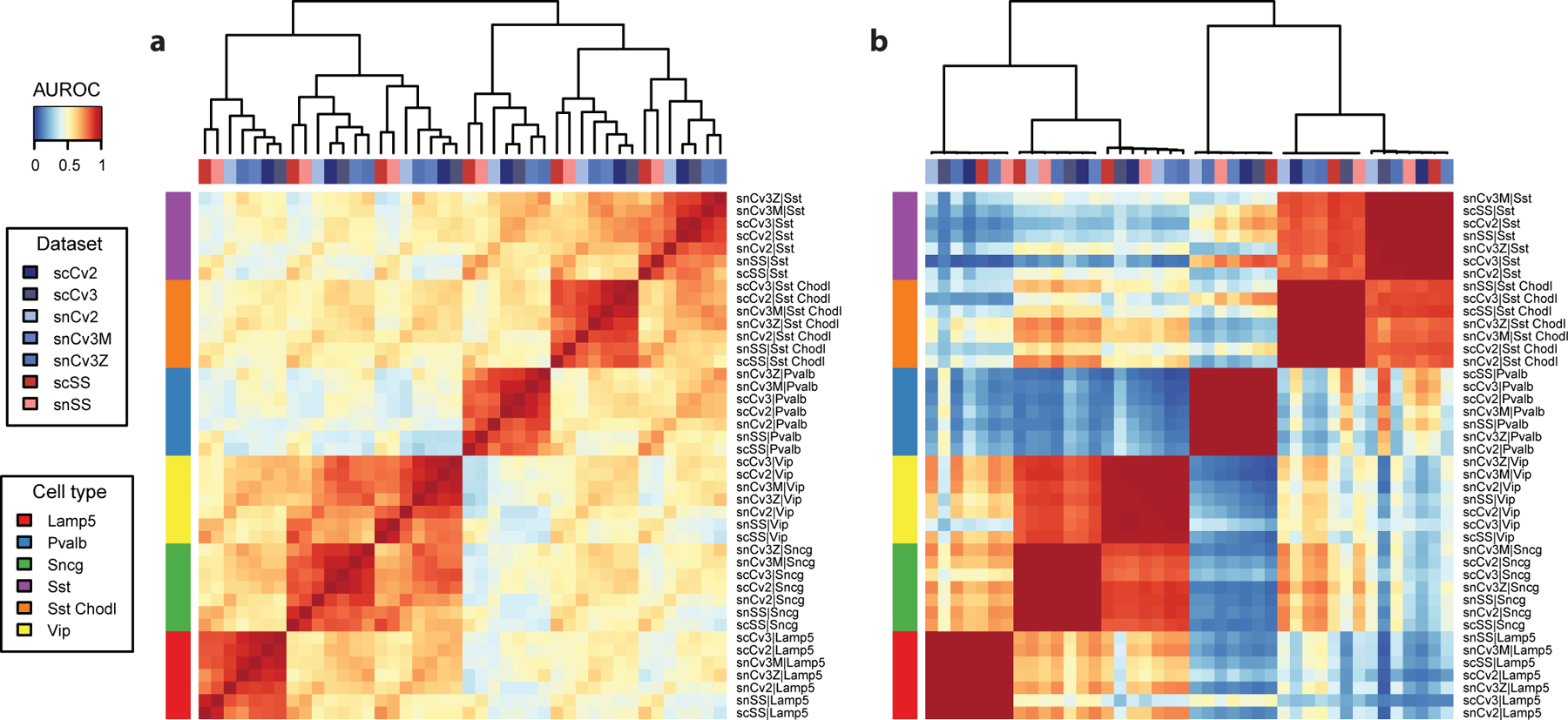
a Possible issue: Spearman correlation of cell type centroids is affected by technical variability. The heatmap shows some evidence of replicating cell types (light red rectangles), but is dominated by batch effects, largely obscuring secondary relationships between cell types. Red colors correspond to datasets using the Smart-Seq technology, blue colors to datasets using the 10x technology, light colors to single nuclei datasets, dark colors to single cell datasets. b Anticipated result: MetaNeighbor AUROCs alleviate most of the concerns seen in a, with clear groups of replicating cell types (dark red squares, AUROC ~ 1) and clear secondary relationships (e.g., similarity of CGE-derived interneurons Vip, Sncg and Lamp5).

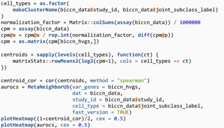
Compared to correlations, AUROCs have one additional “parameter”: the outgroup used for the prediction task. In Procedure 1, we illustrated how the outgroup can be controlled and interpreted. A deviation from AUROC = 1 can thus be interpreted as a combination of two factors: lack of similarity between cell types and choice of outgroup (difficulty of prediction task). If the outgroup is well controlled, AUROC values will generalize across studies and fundamentally indicate the quality of the clustering. For a given cell type in a given background (for example Sst cells in an unbiased sample of primary motor cortex inhibitory neurons), the similarity to Sst cells in another dataset (or any other inhibitory type for that matter) should be in the range of similarity observed within the BICCN.

As a robust alternative to centroid correlations, MetaNeighbor AUROCs can be applied to simple preprocessing tasks, such as identifying and selecting cell types that overlap between datasets before applying a merging framework. However, beyond the purely applicative viewpoint, we believe that MetaNeighbor-style AUROCs are a stepping stone toward a generalizable formalization of cell type similarity.

Data availability

The datasets analyzed in the protocol are all previously published and publicly available:

• Human pancreas datasets: from Baron et al.³² (GEO accession code GSE84133), Lawlor et al.³³ (GEO accession code GSE86473), Muraro et al.³⁴ (GEO accession code GSE85241), and Segerstolpe et al.³⁵ (ArrayExpress accession code E-MTAB-5061). These datasets are accessed through the Bioconductor scRNAseq library in the protocol.

• Mouse primary visual cortex dataset from Tasic et al.³⁶ (GEO accession code GSE71585), accessed through the Bioconductor scRNAseq library.

• The Brain Initiative Cell Census Network (BICCN) dataset for the mouse primary motor cortex from Yao et al.⁴ is available on the NeMO archive (https://assets.nemoarchive.org/dat-ch1nqb7). The subset of the BICCN data necessary to run the protocol is also available on FigShare at https://doi.org/10.6084/m9.figshare.13020569 (R version) and https://doi.org/10.6084/m9.figshare.13034171 (Python version).

References

- 1.Hay SB, Ferchen K, Chetal K, Grimes HL & Salomonis N The Human Cell Atlas bone marrow single-cell interactive web portal. Exp. Hematol 68, 51–61 (2018). [DOI] [PMC free article] [PubMed] [Google Scholar]
- 2.Schaum N et al. Single-cell transcriptomics of 20 mouse organs creates a Tabula Muris. Nature 562, 367–372 (2018). [DOI] [PMC free article] [PubMed] [Google Scholar]
- 3.Almanzar N et al. A single-cell transcriptomic atlas characterizes ageing tissues in the mouse. Nature 583, 590–595 (2020). [DOI] [PMC free article] [PubMed] [Google Scholar]
- 4.Yao Z et al. An integrated transcriptomic and epigenomic atlas of mouse primary motor cortex cell types. bioRxiv 2020.02.29.970558 (2020) doi: 10.1101/2020.02.29.970558. [DOI] [Google Scholar]
- 5.Yao Z et al. A taxonomy of transcriptomic cell types across the isocortex and hippocampal formation. bioRxiv 2020.03.30.015214 (2020) doi: 10.1101/2020.03.30.015214. [DOI] [PMC free article] [PubMed] [Google Scholar]
- 6.Bakken TE et al. Evolution of cellular diversity in primary motor cortex of human, marmoset monkey, and mouse. bioRxiv 2020.03.31.016972 (2020) doi: 10.1101/2020.03.31.016972. [DOI] [Google Scholar]
- 7.Duò A, Robinson MD & Soneson C A systematic performance evaluation of clustering methods for single-cell RNA-seq data. F1000Research 7, 1141 (2018). [DOI] [PMC free article] [PubMed] [Google Scholar]
- 8.Haghverdi L, Lun ATL, Morgan MD & Marioni JC Batch effects in single-cell RNA-sequencing data are corrected by matching mutual nearest neighbors. Nat. Biotechnol 36, 421–427 (2018). [DOI] [PMC free article] [PubMed] [Google Scholar]
- 9.Stuart T et al. Comprehensive Integration of Single-Cell Data. Cell 177, 1888–1902.e21 (2019). [DOI] [PMC free article] [PubMed] [Google Scholar]
- 10.Welch JD et al. Single-Cell Multi-omic Integration Compares and Contrasts Features of Brain Cell Identity. Cell 177, 1873–1887.e17 (2019). [DOI] [PMC free article] [PubMed] [Google Scholar]
- 11.DePasquale EAK et al. cellHarmony: cell-level matching and holistic comparison of single-cell transcriptomes. Nucleic Acids Res. 47, e138–e138 (2019). [DOI] [PMC free article] [PubMed] [Google Scholar]
- 12.Hie B, Bryson B & Berger B Efficient integration of heterogeneous single-cell transcriptomes using Scanorama. Nat. Biotechnol 2019 1 (2019) doi: 10.1038/s41587-019-0113-3. [DOI] [PMC free article] [PubMed] [Google Scholar]
- 13.Barkas N et al. Wiring together large single-cell RNA-seq sample collections. bioRxiv 460246 (2018) doi: 10.1101/460246. [DOI] [Google Scholar]
- 14.Luo C et al. Single nucleus multi-omics links human cortical cell regulatory genome diversity to disease risk variants. bioRxiv 2019.12.11.873398 (2019) doi: 10.1101/2019.12.11.873398. [DOI] [PMC free article] [PubMed] [Google Scholar]
- 15.Crow M, Paul A, Ballouz S, Huang ZJ & Gillis J Characterizing the replicability of cell types defined by single cell RNA-sequencing data using MetaNeighbor. Nat. Commun 9, 884 (2018). [DOI] [PMC free article] [PubMed] [Google Scholar]
- 16.Paul A et al. Transcriptional Architecture of Synaptic Communication Delineates GABAergic Neuron Identity. Cell 171, 522–539.e20 (2017). [DOI] [PMC free article] [PubMed] [Google Scholar]
- 17.Hodge RD et al. Conserved cell types with divergent features in human versus mouse cortex. Nature 573, 61–68 (2019). [DOI] [PMC free article] [PubMed] [Google Scholar]
- 18.Butler A, Hoffman P, Smibert P, Papalexi E & Satija R Integrating single-cell transcriptomic data across different conditions, technologies, and species. Nat. Biotechnol (2018) doi: 10.1038/nbt.4096. [DOI] [PMC free article] [PubMed] [Google Scholar]
- 19.Forcato M, Romano O & Bicciato S Computational methods for the integrative analysis of single-cell data. Brief. Bioinform bbaa042 (2020) doi: 10.1093/bib/bbaa042. [DOI] [PMC free article] [PubMed] [Google Scholar]
- 20.Hie B et al. Computational Methods for Single-Cell RNA Sequencing. Annu. Rev. Biomed. Data Sci 3, null (2020). [Google Scholar]
- 21.Tran HTN et al. A benchmark of batch-effect correction methods for single-cell RNA sequencing data. Genome Biol. 21, 12 (2020). [DOI] [PMC free article] [PubMed] [Google Scholar]
- 22.Luecken MD et al. Benchmarking atlas-level data integration in single-cell genomics. bioRxiv 2020.05.22.111161 (2020) doi: 10.1101/2020.05.22.111161. [DOI] [PMC free article] [PubMed] [Google Scholar]
- 23.Abdelaal T et al. A comparison of automatic cell identification methods for single-cell RNA sequencing data. Genome Biol. 20, 194 (2019). [DOI] [PMC free article] [PubMed] [Google Scholar]
- 24.Kiselev VY, Yiu A & Hemberg M scmap: projection of single-cell RNA-seq data across data sets. Nat. Methods 15, 359–362 (2018). [DOI] [PubMed] [Google Scholar]
- 25.Büttner M, Miao Z, Wolf FA, Teichmann SA & Theis FJ A test metric for assessing single-cell RNA-seq batch correction. Nat. Methods 16, 43–49 (2019). [DOI] [PubMed] [Google Scholar]
- 26.Kapp AV & Tibshirani R Are clusters found in one dataset present in another dataset? Biostatistics 8, 9–31 (2007). [DOI] [PubMed] [Google Scholar]
- 27.Dudoit S, Fridlyand J & Speed TP Comparison of Discrimination Methods for the Classification of Tumors Using Gene Expression Data. J. Am. Stat. Assoc 97, 77–87 (2002). [Google Scholar]
- 28.Kiselev VY et al. SC3: consensus clustering of single-cell RNA-seq data. Nat. Methods 14, 483–486 (2017). [DOI] [PMC free article] [PubMed] [Google Scholar]
- 29.Tasic B et al. Shared and distinct transcriptomic cell types across neocortical areas. Nature 563, 72–78 (2018). [DOI] [PMC free article] [PubMed] [Google Scholar]
- 30.gillislab/MetaNeighbor-Protocol. (gillislab, 2020). [Google Scholar]
- 31.Protocol data (R version). (2020) https://doi.org/doi: 10.6084/m9.figshare.13020569.v2. [DOI] [Google Scholar]
- 32.Baron M et al. A Single-Cell Transcriptomic Map of the Human and Mouse Pancreas Reveals Inter- and Intra-cell Population Structure. Cell Syst. 3, 346–360.e4 (2016). [DOI] [PMC free article] [PubMed] [Google Scholar]
- 33.Lawlor N et al. Single-cell transcriptomes identify human islet cell signatures and reveal cell-type-specific expression changes in type 2 diabetes. Genome Res. 27, 208–222 (2017). [DOI] [PMC free article] [PubMed] [Google Scholar]
- 34.Muraro MJ et al. A Single-Cell Transcriptome Atlas of the Human Pancreas. Cell Syst. 3, 385–394.e3 (2016). [DOI] [PMC free article] [PubMed] [Google Scholar]
- 35.Segerstolpe Å et al. Single-Cell Transcriptome Profiling of Human Pancreatic Islets in Health and Type 2 Diabetes. Cell Metab. 24, 593–607 (2016). [DOI] [PMC free article] [PubMed] [Google Scholar]
- 36.Tasic B et al. Adult mouse cortical cell taxonomy revealed by single cell transcriptomics. Nat. Neurosci 19, 335–346 (2016). [DOI] [PMC free article] [PubMed] [Google Scholar]
Related links
Key references using this protocol
- Crow M et al. Nat Commun 9, 884 (2018): 10.1038/s41467-018-03282-0 [DOI] [PMC free article] [PubMed] [Google Scholar]
- Paul A et al. Cell 171, 522–539.e20 (2017): 10.1016/j.cell.2017.08.032 [DOI] [PMC free article] [PubMed] [Google Scholar]
- Yao Z et al. bioRxiv 2020.02.29.970558 (2020): 10.1101/2020.02.29.970558 [DOI] [Google Scholar]
- Bakken TE et al. bioRxiv 2020.03.31.016972 (2020): 10.1101/2020.03.31.016972 [DOI] [Google Scholar]
Key data used in this protocol
- Baron M et al. Cell Syst. 3, 346–360.e4 (2016): 10.1016/j.cels.2016.08.011 [DOI] [PMC free article] [PubMed] [Google Scholar]
- Lawlor N et al. Genome Res. 27, 208–222 (2017): 10.1101/gr.212720.116 [DOI] [PMC free article] [PubMed] [Google Scholar]
- Muraro MJ et al. Cell Syst. 3, 385–394.e3 (2016): 10.1016/j.cels.2016.09.002 [DOI] [PMC free article] [PubMed] [Google Scholar]
- Segerstolpe Å et al. Cell Metab. 24, 593–607 (2016): 10.1016/j.cmet.2016.08.020 [DOI] [PMC free article] [PubMed] [Google Scholar]
- Tasic B et al. Nat. Neurosci 19, 335–346 (2016): 10.1038/nn.4216 [DOI] [PMC free article] [PubMed] [Google Scholar]
Associated Data
This section collects any data citations, data availability statements, or supplementary materials included in this article.
Data Availability Statement