Improving Phylogenies Based on Average Nucleotide Identity, Incorporating Saturation Correction and Nonparametric Bootstrap Support

Abstract

Whole-genome comparisons based on average nucleotide identities (ANI) and the genome-to-genome distance calculator have risen to prominence in rapidly classifying prokaryotic taxa using whole-genome sequences. Some implementations have even been proposed as a new standard in species classification and have become a common technique for papers describing newly sequenced genomes. However, attempts to apply whole-genome divergence data to the delineation of higher taxonomic units and to phylogenetic inference have had difficulty matching those produced by more complex phylogenetic methods. We present a novel method for generating statistically supported phylogenies of archaeal and bacterial groups using a combined ANI and alignment fraction-based metric. For the test cases to which we applied the developed approach, we obtained results comparable with other methodologies up to at least the family level. The developed method uses nonparametric bootstrapping to gauge support for inferred groups. This method offers the opportunity to make use of whole-genome comparison data, that is already being generated, to quickly produce phylogenies including support for inferred groups. Additionally, the developed ANI methodology can assist the classification of higher taxonomic groups.[Average nucleotide identity (ANI); genome evolution; prokaryotic species delineation; taxonomy.]

DNA–DNA hybridization holds the distinction of being the gold standard for prokaryotic species delineation (Stackebrandt and Goebel 1994). The method is technically challenging and its results at times are poorly reproducible across labs (Grimont et al. 1980; Huss et al. 1983). Consequently, ongoing efforts attempt to supplement or replace DNA–DNA hybridization with in silico methods by taking advantage of the ongoing revolution in genome sequencing (Konstantinidis and Tiedje 2005; Goris et al. 2007; Auch et al. 2010; Colston et al. 2014; Varghese et al. 2015). One of the major approaches has been average nucleotide identity (ANI) (Konstantinidis and Tiedje 2005).

ANI was first proposed in 2005. At the time the method used the average nucleotide identity of shared open reading frames (ORFs) instead of the whole-genome (Konstantinidis and Tiedje 2005). The authors defined a species-level ANI cutoff and examined large disparities in gene content among the strains and species in their data set. A year later, they explored this metric in greater depth and observed that ANI was correlated with the percent of content shared, but that a large amount of genomic nucleotide divergence (1–2%) needed to have occurred before there were major shifts in genome content (Konstantinidis et al. 2006). In 2007, the emphasis shifted from ORFs to the whole genome as the ANI method was adapted to directly compare to DNA–DNA hybridization (Goris et al. 2007). This shift led to the development of programs such as the jSpecies Java application which could perform the Goris method in a local and scalable manner (Richter and Rosselló-Móra 2009). However, the consideration of the varying gene content became de-emphasized with the default exportable output from jSpecies not including any reference to shared content in comparisons. This de-emphasis on gene content is largely irrelevant when comparing closely related organisms due to the correlation between ANI and shared genome content. Yet, this becomes a problem when only fractions of the genomes are shared; this can lead to spurious ANI results.

The problem of shared gene content was examined again in 2015 with the publication of the gANI method (Varghese et al. 2015). This approach explicitly considers the shared gene content and offers two separate delimiters for a species: gANI (global ANI, which was based on the 2005 method), as well as an “Alignment Fraction” (AF), a measure of the proportion of genes shared. While gANI offers an important upgrade to the ANI paradigm it does contain an important limitation. Namely, there is no obvious answer on how to interpret a comparison between two taxa where the ANI is above the threshold and the AF is below, or vice versa, which is a problem given that these metrics are most often used for species delimitation in prokaryotes. It should be noted here that this problem has also been tackled, in part with the Genome-to-Genome Distance Calculator (GGDC) (Henz et al. 2005). The GGDC provides whole-genome measures directly on the same scale as DNA–DNA hybridization, effectively incorporating sequence identity and alignment fraction.

Here we suggest that ANI-derived distance measures can also be used to reconstruct prokaryotic phylogenies that reflect shared ancestry, thus providing a natural extension to group species into genera and families. We introduce a single distance measure from whole-genome data incorporating both the ANI and AF, labeled Total Average Nucleotide Identity (tANI), into the final metric. An advantage of the described method is that it can be applied to high-quality draft genomes prior to annotation and gene clustering. Additional time is saved by using distance-based tree-building methods that are typically faster than maximum-likelihood or Bayesian inference methods. Ignoring phylogenetic information retained in individual gene families, this approach is not impacted by gene transfers that create misleading phylogenetic information—a gene acquired from outside the studied group will lower the alignment fraction, but it will not provide a large signal moving the gene recipient closer to the root of the studied group. Furthermore, including the AF in the calculation of pairwise distances incorporates gene transfers as a process of genome divergence by actively affecting the summed AF’s value, and its subsequent impact on the overall distance measure. We correct pairwise distances for saturation and use bootstrap resampling to assess support. The analyzed test cases illustrate that this approach reliably resolves relationships within genera and families. We also test the methodology on a small group of eukaryotes to investigate the feasibility of this method within that group and find that the approach works well in sampled yeast genomes.

Methods

Genomes Used

The genomes used in this study are either high-quality draft whole-genome assemblies or complete assemblies available via NCBI (Supplementary Table S1 available on Dryad at https://doi.org/10.5061/dryad.jwstqjq85). These genomes were grouped into 4 different data sets that largely correspond to the following groups: Aeromonas, Rhodobacterales, Frankiales, and Aeromonadales (extended with members of the Enterobacteriales). Initially, no completion criterion was used; however, phylogenies built from genomes with very low completion scores (as measured by CheckM; Parks et al. 2015) were questionable at best, and these genomes were thrown out in the early stages of method development. Genomes used in this study are all above 88% completion (sans 1 genome from the Aeromonadales data set) and most are above 98%. Selection initially centered on two groups for which previous phylogenetic and phylogenomic work had been done by us. The first, the Aeromonas data set, encompasses the 56 Aeromonas genomes used in Colston et al. (2014) and represents a genus-level taxonomic unit. Aeromonas is a genus of free-living or host-associated gammaproteobacteria. Many strains cause disease in animals; however, beneficial associations were described in fish and leeches (Gonçalves Pessoa et al. 2019). The delineation and phylogeny of Aeromonas species were revised using whole-genome and multilocus sequence analyses (Colston et al. 2014; Fernández-Bravo and Figueras 2020). This data set was chosen principally on the fact that the Aeromonas are known to undergo large amounts of horizontal gene transfer, which allows them to serve as a control against the influence of such events (Morandi et al. 2005; Silver et al. 2011; Colston et al. 2014; Kloub et al. 2021).

The Rhodobacterales data set encompasses alphaproteobacterial genera used in Collins et al. (2015) and Gromek et al. (2016) plus additional genomes to investigate the monophyletic nature of Loktanella and Ruegeria (Collins et al. 2015; Gromek et al. 2016). This data set provided the opportunity to test the paraphyletic nature of the clades within the group as seen in Collins et al. 2015. This set corresponds closely to a family-level taxonomic unit (exempting the genera: Phenylobacterium, Parvularcula, Maricaulis, Hyphomonas, Hirschia, Caulobacter, Brevundimonas, and Asticcacaulis, which are used as outgroups to root the phylogeny). A third set, aimed at encompassing a broader phylogenetic and taxonomic range, was created by adding all publicly available non-Aeromonas Aeromonadales genomes to a subset of the Aeromonas data set along with taxa outside the order including members of the Enterobacteriales. All together this group is referred to as the Aeromonadales data set, and, as the name implies, it corresponds to an order-level unit. This group provided the opportunity to examine tANI across the order threshold by looking at members of the Enterobacteriales and their relationships to the Aeromonadales. Furthermore, we were able to include previously unknown and unsequenced members of the Aeromonadales in a phylogenetic analysis.

The available genomes from the order Frankiales were formed into another data set (of the same name). The Frankiales, an order of actinobacteria, contain mostly nitrogen-fixing symbionts of pioneer plants (Normand and Fernandez 2021). The group is known for its tremendous variation in genome size and GC-contents (Normand et al. 2007) and was used to test the robustness of the tANI method towards variation of these factors (Nouioui et al. 2016a, 2016b; Tisa et al. 2016; Normand et al. 2018).

Finally, the Yeast data set was built from a small selection of Saccharomyces whole genomes including five separate species (cerevisiae, kudriavzevii, pastorianus, bayanus, and uvarum). The primate data set was similarly built out of whole genomes for several primate species and one mouse whole genome. All whole genomes were sourced from NCBI (see Supplementary Table S6 available on Dryad for accession numbers).

Reference Phylogenies

Reference phylogenies for comparison were obtained or generated for each data set. For Aeromonas, the multilocus sequence alignment (MLSA) and expanded core phylogenies were obtained from Colston et al. (2014). A reference for the Rhodobacterales data set was generated by replicating the method described in Collins et al. (2015) but with added Loktanella and Ruegeria genomes from NCBI. The Aeromonadales reference phylogeny was calculated by following the MLSA methodology described in Colston et al. (2014) for the included genomes (Colston et al. 2014).

The Frankiales reference required the de novo creation of an MLSA scheme in the absence of thorough examples in the literature. Twenty-four single-copy housekeeping genes were selected to form the alignment (Supplementary Table S5 available on Dryad). Nucleotide sequences for each gene were retrieved via BLAST from Frankia casuarinae (Accession: NC_007777.1). BLASTn (v2.6.0) (Altschul et al. 1990) was executed with the gene sequences as the query and the genomes as the target sequence. The coding sequences corresponding to the highest scoring hits (using e-values) for each gene in a singular genome were aligned and concatenated. This was repeated for every genome, generating the MLSA file. IQTree (v1.5.5) was executed with the MLSA file and built the phylogenetic tree with 1000 ultrafast bootstraps (Nguyen et al. 2015; Chernomor et al. 2016; Kalyaanamoorthy et al. 2017; Hoang et al. 2018). IQTree’s ModelFinder arrived at the SCHN05 empirical codon model with empirical codon frequencies (F) and Free Rate (Soubrier et al. 2012) model of rate heterogeneity with nine categories (R5).

ANI and AF Calculation

Our ANI and BLAST methodology differs from Varghese et al. (2015) in two respects. First, we do not limit our search to open reading frames but rather use the full scaffold/contig set of an organism. Second, we fracture the genomes into 1,020 nucleotide fragments in line with previous iterations of ANI calculation (Konstantinidis and Tiedje 2005; Richter and Rosselló-Móra 2009). The fragments from the query genome were each compared to the whole reference genome via BLAST (v2.7.1). BLAST results were filtered based on coverage, percent identity, and e-values (1E4 cutoff), and only the top best hit (of query fragment versus reference genome) was retained per fragment (for more information on thresholds see: Coverage and percent identity cutoffs section). Filtered results were used to calculate the ANI and AF.

ANI is calculated in a similar methodology to that described by Varghese et al. (2015) such that ANI is not simply the sum of best-hit identities over the total number of genes, but is instead described by the formula: ANI (ID%*Length of Alignment)/( (Length of the shorter fragment). Alignment fraction is described as: (Length of the shorter fragment)/(Length of the Query Genome). The ID%, Length of the Alignment, and Length of the shorter fragment terms refer to the individual blast hits from genome–genome comparisons (see above).

The distance (abbreviated Total Average Nucleotide Identity, or tANI) was calculated by using the formula: tANI -ln(AF*ANI). The natural log added to this calculation counteracts saturation for low AF*ANI values.

A perl script which runs the tANI protocol can be found at https://github.com/SeanGosselin/tANI_Matrix. It will produce the distance matrices needed for tree building.

Bootstrap Replicates

After genomes were split into 1020 nucleotide segments, individual 1020 nucleotide segments were chosen randomly with replacement and used to create a new data set of fragments for that genome. This new 1020 fragment data set was then compared against all other genomes using the tANI methodology to create a row on the bootstrapped matrix. This process is then repeated on all genomes to fill out the matrix. This matrix was then used to infer a tree. The process is repeated for the number of bootstraps desired, and then those trees were mapped onto the best tree to provide node support values.

Coverage and Percent Identity Cutoffs

The original percent identity and coverage cutoff values were chosen based on those laid down by Varghese et al. (2015). Cutoff values were tested within the Aeromonas data set. Average distance within the clade was measured over a range of cutoff values (Supplementary Fig. S1 available on Dryad) and multiple potential cutoffs were tested against the jSpecies ANI standard cutoffs of 70% identity and 70% length. We tested various cutoff values’ ability to construct phylogenetic trees compared to more conventional methods and concluded that 70-at-70 produced phylogenies most similar to our reference trees.

Phylogenies from Distances

Tree-building from distance matrices was accomplished using the R packages Ape and Phangorn (Paradis et al. 2004; Schliep 2011). The balanced minimum evolution algorithm as implemented in the FastME function of APE was used to generate phylogenies for each distance matrix (Desper and Gascuel 2002). Parameters used were: nni TRUE, spr TRUE, tbr TRUE. A “best tree” was calculated from the point estimate values (the initial calculated distance matrix in tANI) and a collection of bootstrap topologies from the resampled matrices. Support values were mapped onto the best tree using the function plotBS in Phangorn (Schliep 2011). The R script used to create the phylogenies from our distance matrices is also available: https://github.com/SeanGosselin/tANI_Matrix.

Split graphs were constructed from the distance matrices using Splitstree4 (Huson and Bryant 2006) and were included to provide an assessment on how tree-like or tree compatible our distance matrices are. Graphs were built using a NeighborNet distance transformation, ordinary least squares variance, and a lambda fraction of 1.

To evaluate our bootstraps, tree certainty scores were calculated using the IC/TC score calculation algorithm implemented in RAxML v8 (Salichos et al. 2014; Stamatakis 2014). Tree distances were calculated using the R package Ape (Paradis et al. 2004) and the treedist function of Phangorn (Schliep 2011).

Receiver Operating Characteristic Curve Analysis

A receiver operating characteristic (ROC) curve was used to determine the optimal species cutoff for a single genome-to-genome distance calculation. Genomes from the sets of Aeromonadales and Rhodobacterales listed in the genome table were compiled and matrices of both the distance and raw jSpecies ANI were compiled from the set. The jSpecies ANI values were used to delimit species from the genomes selected. Each comparison was assigned a 1 if the comparison met the species cutoff, and a 0 if it did not according to jSpecies cutoffs (Richter and Rosselló-Móra 2009). This list of 1’s and 0’s represents the true state.

True states and distance values were then compiled into a two-column data set. The R package pROC (Robin et al. 2011) allowed us to create a curve from the data and then determine the best cutoff values for the given set of data such that true negatives and true positives based on the cutoff value were maximized using methodology previously described (Youden 1950).

Average Amino Acid (AAI) Identity

AAI values for Figure 1B were all calculated using the CompareM software package (Parks 2021). Specifically, the aai_wf, and blastp options were used such that they were comparable to the blast-based tANI. Mean AAI values were extracted using in-house R scripts and plotted against the corresponding patristic distance.

Figure 1.

tANI distance value as a function of uncorrected jSpecies ANI value (a). This plot comprises individual genome-genome comparisons from both the Aeromonadales and Rhodobacterales data sets, resulting in a data set of 6195 comparisons. This “tornado” configuration illustrates that jSpecies ANI deviates from a linear relationship as the ANI values drop below 85%. This saturation is a function of declining AF values and sequence substitutions. To further illustrate the point tANI, 1-ANI*AF, 1-ANI, ln(AAI), and 1-AAI were compared using the Frankiales data set (b). Distance values for all genome-genome comparisons were plotted on the Y axis while the corresponding patristic distance (derived from the Frankiales MLSA phylogeny) between the two leaf nodes for that comparison was plotted on the X.

Results

Necessity of Saturation Correction and AF Incorporation

ANI values and the programs that calculate them were not designed with the intent of phylogenetic reconstruction. Consequently, the basic methodology works well within the confines of species delineation; however, the ANI values (or the corresponding sequence divergence) become prone to saturation and lose information when one attempts to compare more divergent taxa. To illustrate this, we took two of our data sets, the Rhodobacterales and the Aeromonadales (Table 1) (see Supplementary Table S01 available on Dryad for a detailed description of the data sets) and compared the ANI values calculated from JSpecies (Richter and Rosselló-Móra 2009) to our tANI method (Fig. 1a).

Table 1.

Abridged data set descriptions.

Data set	Composition	Remarks
Aeromonas	Drawn from Colston, Fullmer et al. 2014. Only has Aeromonas genomes.	Chosen as these genomes already had MLSA and core genome phylogenetic trees constructed, allowing for us to more easily compare our method to these.
Aeromonadales	Composed of several Aeromonas genomes, the remaining available Aeromonadales outside of the Aeromonas, and several Enterobacterales which served as an outgroup.	With genomes from two separate orders, this data set provides opportunity to explore outer limits of the method in regards to taxonomic range.
Rhodobacterales	Consists of Rhodobacterales genomes with a leaning towards the genera Leisingera, Loktanella, and Ruegeria.	Chosen for familiarity and for previously made MLSA for a subset of the taxa which provided an easy route for expansion.
Frankiales	Consists of a selection of publicly available Frankiales genomes.	Selected for the variety of genome sizes and GC content present within the Order, allowing us to check for biases.

Based on dominant taxa in the data set.

A more comprehensive breakdown of the data set is available in Supplementary material available on Dryad.

As genome comparisons move away from the within-species scale that ANI was designed for (Konstantinidis and Tiedje 2005) the noise in the jSpecies ANI result becomes considerable. In extreme cases, the jSpecies ANI value for a comparison can border on the species cutoffs despite incorporating only a small fraction of the genomes. An example of this occurs in the Aeromonadales data set. Aeromonas bivalvium CECT 7113T is found to have jSpecies ANI values around 94% when compared to Aeromonas media CECT 4232T; however, the AF has a value of only 0.527 (far below the expected species cutoff). The effects of small alignment fraction and no correction for saturation is further illustrated in the topology of a distance tree inferred from uncorrected jSpecies ANI values (Fig. 2). These results from the Aeromonadales data set clearly demonstrate the effect of saturation on phylogenetic reconstruction beyond the most closely related of taxa. Through incorporation of AF into the pairwise distance and correcting for saturation, the tANI method ameliorates the issues described above. This is demonstrated by a comparison of tANI to 1-ANI, 1-ANI*AF, and the closely related AAI metrics, and plotting them against the patristic distance between corresponding nodes on the Frankiales MLSA phylogeny (Fig. 1b). The 1-ANI measure rapidly enters into saturation as the patristic distance between tips increases; however, the 1-ANI*AF measure performs better, discerning more information across phylogenetic distance. This is shown especially clearly when the ANI*AF metric is log transformed; the new tANI metric ends up being largely linear with respect to phylogenetic distance. Furthermore, it is clear that although AAI competes very well against ANI alone, it does not perform as well as tANI across longer phylogenetic distances (for a paneled version of 1b, with different axes see Supplementary Fig. S2 available on Dryad). Using jSpecies ANI with the MUMmer algorithm, the saturation effects appear even earlier (Kurtz et al. 2004; Richter and Rosselló-Móra 2009). We want to emphasize that our comparison with uncorrected ANI values should not be seen as a criticism of the original ANI methods, rather we use the comparison to illustrate the importance of considering AF and saturation in case ANI is used to infer shared ancestry.

Figure 2.

FastME phylogenies of the same Aeromonadales data set. a) The phylogeny inferred from jSpecies ANI values, converted to the uncorrected distances (100-%ANI) depicted on the scale bar. The highlighting on A reflects the location of members from the Aeromonas genus within the data set. b) The phylogeny on the right is created from the same data set using the tANI methodology before using FastME. All Aeromonas members are highlighted to illustrate their placement as a single clade. The scale bar depicts length of the branches in tANI distance.

Genome Size and GC Content Do Not Create a Detectable Bias

Since our distance measure is based on the whole genome, differences in genomic traits, such as size and GC-content, could bias the results of the calculations and introduce artifacts into the final phylogeny and their support values. To test this, we developed a data set using the order Frankiales (Table 1), composed primarily of the genus Frankia. This group has high variance in genome size ( 4 Mb to 11 Mb) and considerable range of GC-contents ( 60% to 75%) which made it an ideal test case.

The tANI-based distance tree for the Frankiales (Fig. 3b) set was very similar to the MLSA-derived (multilocus sequence alignment) reference phylogeny (Fig. 3a) (see the Accuracy of the tANI methods compared to multi-gene methods section for a more detailed analysis). Mapping the size of the genome onto the tANI phylogeny showed no pattern of clustering by genome size (Supplementary Fig. S3a available on Dryad). While some groups cluster with similar sizes (e.g., the F. coriariae and F. alni clades), they match the MLSA topology and do not consistently group with only similar-sized genomes. Mapping the GC-content onto the tANI phylogeny produced a similar result (Supplementary Fig. S3b available on Dryad), with no obvious patterns of GC-content bias.

Figure 3.

Phylogenies of the Frankiales data set using two different methodologies. a) The tANI derived phylogeny (left) compared against b) the MLSA phylogeny (right). See Materials and Methods for details on the methods used phylogenetic reconstruction. Scale bars depict tANI distance (a) and substitutions per site (b).

Bootstrap Confidence Sets for tANI and Core Genome ML Analyses are Similar

To provide support values for our distance-based phylogenies, our script creates a set of nonparametric bootstrapped distance matrices (see material and methods for details). Internode certainty (IC) scores were calculated to assess the statistical uncertainty of the trees derived from nonparametric bootstrapping (in the following labeled as “support sets”). IC scores were calculated by mapping statistical support sets against reference trees (the tree derived from the original data without bootstrapping) as implemented in RAxML v8.1 (Salichos et al. 2014; Stamatakis 2014). IC represents a quantification of the level of disagreement in a support set for a particular node in a phylogeny; a higher score indicates less disagreement between topologies. The tree certainty average (TCA) value is the average of IC values across the entire tree, representing an assessment of overall conflict between the support set and reference phylogeny (Salichos et al. 2014). The Aeromonas data set (Table 1) was used as a test case as it offers an expanded core phylogeny in addition to the MLSA, allowing a comparison between different whole-genome methods. Comparing support data sets against the best tree calculated using the same method, the TCA for the Aeromonas tANI phylogeny was 0.86, 0.87 for the expanded core genome phylogeny, and 0.65 for the MLSA phylogeny. Comparing between approaches (MLSA, tANI, Mashtree) results in positive TCAs, that is the trees agree with one another more than they disagree; however, the scores are below 0.4, with the exception of tANI and core genomes based analyses for the Aeromonas data set, which resulted in TCAs of 0.61 (Supplementary Table S2 available on Dryad). To further compare our bootstrap method to other approaches, we calculated the Robinson–Foulds distances within each of the support sets from the MLSA and tANI method and analyzed the pairwise distances using principal coordinate analysis (PCoA) (Fig. 4). The PCoA plot shows that the statistical support sets for both data sets colocalize with one another; indicating that the support sets from the different methods represent similar tree space.

Figure 4.

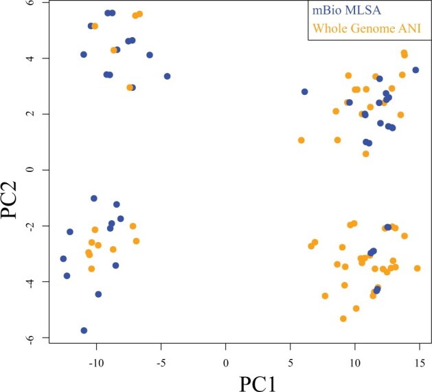
PCoA plot of the distance between trees from bootstrap samples calculated from the Aeromonas core genome, and tANI methods. The samples from the tANI method are listed in the key as Whole Genome ANI, and the Aeromonas core genome bootstraps are in the key as mBio MLSA. The support sets overlap in every cluster, suggesting that the two methods capture similar topologies.

Accuracy of the tANI Methods Compared to Multigene Methods

For the Aeromonas test data set, differences between the extended core phylogeny and the tANI derived phylogeny are the placements of Aeromonas veronii AMC34 and the Aeromonas allosaccharophila clade (Fig. 5). Aeromonas veronii AMC 34 is still placed within the extended A. veronii, Aeromonas sobria, and A. allosaccharophila clade using the tANI method, but tANI disagrees on the specific location, and places AMC 34 sister to the A. veronii group, instead of sister to the entire clade. This placement as sister to the veronii group shifts the placement of the A. allosaccharophila and A. sobria strains especially in regard to the placement of Aeromonas fluviasis and Aeromonas australiensis. However, AMC 34’s placement is poorly supported in the tANI-based analysis. Deeper clades within the tANI phylogeny match those of the extended core phylogeny and are highly supported.

Figure 5.

Comparison of Aeromonas phylogenies reconstructed using different methodologies. a) The Extended Core Phylogeny, inferred using Approximate Maximum-likelihood (Colston et al. 2014), and b) the tANI methodology, inferred using Fast Minimum Evolution. Keys for node support apply to the tree directly to the right of the key. Arrows point to the location of Aeromonas veronii AMC 34. Scale bars depict substitutions per site (a) and tANI distance (b).

The phylogenies produced by the extended core MLSA and tANI for the Frankiales data set also had few differences (Fig. 3). Principal among these was the divergence of clades 2 and 3 since tANI and MLSA disagree over whether clade 2 or clade 3 split off first. There is further disagreement on the placement of individual taxa primarily within clade 2 (see the placement of Frankia sp. Discariae BCU 110501, Frankia spCgIS1, and Frankia spEAN1pec). However, aside from these minor disagreements within the clades, and differing levels of confidence (see bootstrap support, especially within clade 5), these two methods largely reproduce the same phylogeny.

Comparing different methods for the Rhodobacterales data set yielded more complex results (Supplementary Fig. S4 available on Dryad). Both the tANI and the housekeeping gene-based MLSA phylogenies have low levels of support for the internal branches of most of the phylogeny, and disagree on the placement of the genera Ruegeria, Loktanella, Roseobacter, and the several other singletons. The tANI and MLSA trees also disagree on the placement of Loktanella, with the tANI grouping it as one paraphyletic clade broken up by internal nodes and one small monphyletic group, whereas the MLSA method places Loktanella into two separate monophyletic groups. In both cases the same species of Loktanella are grouped together in the smaller monophyletic clades; however, the order of species in the larger clades is more disorganized. tANI and MLSA trees both agree on keeping the Caulobacterales a monophyletic clade, and keep the Leisingera genus together, both with high support. Within Leisingera there is minor disagreement on the placement of the individual strains, but they are largely kept in the same branching pattern. The Ruegeria groupings are also kept intact across the two trees. Further comparison of the tANI-based Rhodobacterales phylogeny against other methods (see Mashtree section below) implies the large amount of internal disagreement is intrinsic to the data set and will require more detailed analysis to untangle. Additional visual confirmation for the results described above is provided by the split graphs created for each of the data sets (see Supplementary Figs. S5–S8 available on Dryad).

Comparison of tANI Method with Mashtree

Genome-based phylogenies have been in the literature for some time. As such, it is appropriate to compare our methodology with other available whole-genome methods and assess our methodology’s strengths and weaknesses. To this end, we first compare our method to Mashtree (Katz et al. 2019), which is an extension of the Mash kmer-calculation (Ondov et al. 2016).

For the Aeromonas data set, Mashtree had only minor disagreements with our method (Supplementary Fig. S9a available on Dryad). For example, MashTree moved the placement of A. media, and shuffled members within the salmonicida and A. aquatica groups. This pattern generally repeats itself in the Rhodobacterales data set (Supplementary Fig. S9b available on Dryad). Mashtree also kept Leisingera, Rhodobacter and the major Ruegeria clade together in a similar fashion to the tANI phylogeny. Additionally, the MashTree phylogeny generally agrees with the branching patterns the tANI phylogeny proposes, while deviating at nodes of low support in the tANI and MSLA based phylogenies. However, Mashtree did separate Loktanella into a number of monophyletic clades. Comparing the Mashtree topology with support sets from tANI, MLSA, and core genome analyses gave results similar to the other TCA values comparing between methods (Supplementary Table S02 available on Dryad).

Also relevant, the updated Genome BLAST Distance Phylogeny (GBDP) software (Meier-Kolthoff et al. 2013), which uses the Genome-to-Genome Distance Calculator (GGDC), has recently been used as part of several studies (García-López et al. 2019; Thorell et al. 2019). The only standalone option implementing GBDP we are aware of is a legacy beta version (http://www.auch-edv.de/GBDP) which does not incorporate the most recent improvements. While this version of GBDP performed well within many genera, it presented strong disagreement within others and across higher taxonomic ranks (Fullmer 2018).

This Novel Extension of ANI Matches Older Methodologies

Since tANI is based off a measure intended for species delimitation, we wanted to see if it maintained this original purpose while also being able to produce phylogenies. To determine the species cutoff based on a single genome-to-genome distance calculation we used a receiver operating characteristic (ROC) curve analysis. Working on the union of the Aeromonas and Rhodobacterales data sets, the ROC estimates a distance cutoff of 0.315, at a specificity (true negative rate) of 99.984 and sensitivity (true positive rate) of 99.200 against the accepted species nomenclature (Fig. 6a). Examination of the ROCs for the constituent data sets reveals that the genera within the two data sets are not equally easy to classify (Fig. 6b,c). However, when taxa in the Rhodobacterales set are reclassified along the lines suggested in the MLSA phylogeny (see Supplementary Table S3 available on Dryad), the genera curve improves in sensitivity from 80% to 99% while maintaining the same specificity (Fig. 6d).

Figure 6.

Receiver operating characteristic curves reporting the sensitivity and specificity of the tANI at discriminating species relationships. Plots show a) the union of the Aeromonas and Rhodobacterales data sets against accepted nomenclature (specificity of 99.98%, and sensitivity of 99.20%), b) the Aeromonas data set (specificity of 96.68%, and sensitivity of 97.97%), c) the Rhodobacterales data set (specificity of 83.78%, and sensitivity of 80.09%), d) the Rhodobacterales data set after reclassifying taxa (specificity of 83.31% and sensitivity of 99.13%).

Novel tANI Method Offers the Ability to Delimit Deeper Taxonomic Ranks

One added benefit from our use of broader taxonomic samplings in some of our data sets is the opportunity to test our distance measure against ANI and GGDC species cutoffs. When the distances for every pair-wise comparison from the Aeromonadales and the Rhodobacterales sets were plotted and filtered for taxa suspected of misclassification (see Supplementary Fig. S10 available on Dryad for a version using NCBI classifications), a series of recognizable peaks for each taxonomic rank were observed (Supplementary Fig. S10 available on Dryad). Most of the peaks were well defined; however, order and class levels coincide and lack a point of separation. The ROCs were used to provide statistical evidence for these observations. At the genus level, the Aeromonadales (Supplementary Fig. S11 available on Dryad) and Rhodobacterales sets (Supplementary Fig. S11b available on Dryad) have similar distance cutoffs (3.3 and 3.4, respectively) and varied but generally high specificities (96.7% and 83.3%) and sensitivities (98.0% and 99.1%). At the family level, the combined data sets returned a cutoff of 4.57 and maintained specificity of 90.7% and sensitivity of 86.5% (Supplementary Fig. S11c available on Dryad). At the order level, the combined data sets fell off to 4.42 cutoff, 94.2% specificity, and 71.44% sensitivity, suggesting the method loses a significant portion of its discriminatory power at this taxonomic rank (Supplementary Fig. S11d available on Dryad). It should be noted that these values are likely to be highly data set specific.

Misclassified Taxa

A number of taxa in our data sets appear to be misclassified under incorrect genus, family, order, and species labels (Supplementary Table S3 available on Dryad). These taxa fall into groups for which phylogenetic analyses also support their misclassification. The ROC determined cutoffs also supported that these taxa are outside of their assigned group. These taxa were reclassified into novel groups along their phylogenetic lines for the purpose of our taxonomic rank cut-off analyses (Supplementary Table S4 available on Dryad). Our tANI metric cutoff agreed with these decisions, and when redoing the ROC analyses with these changes improved the sensitivities and specificities of those cutoffs. There are three specific higher-order classifications to which this applies: Loktanella, Ruegeria, and Succinivibrionaceae. Additionally, several species-level classifications may need to be revised, specifically those mentioned in Supplementary Table S3 available on Dryad.

Tests on Eukaryotic Genomes

We also ran brief tests on two eukaryotic data sets to test the feasibility of using the method outside of prokaryotes (For data set descriptions see Supplementary Table S06 available on Dryad). The first data set, built from whole genomes from one mouse and four primate species, provided inconclusive results. Due to the size of the genomes in question, and the constraint of computational resources available, these runs failed. Analysis of the data set constructed from members of the Saccharomyces resulted in consistent distance measures regardless of which genome was the query or database, and the phylogenetic results were in line with our expectations for genus-level comparisons (Supplementary Fig. S13 available on Dryad).

Discussion

Success of Tree-Building

The tANI method has demonstrated the capacity to match more sophisticated techniques. tANI trees consistently showed comparable levels of conflict to reference phylogenies and matched the level of confidence displayed by other methods such as MLSA when examining the data sets used within this paper. The tANI methodology performed well at the species, genus, family, and order levels; the relationships observed in the reference trees held true in our tANI trees. Furthermore, TCA tests have shown that our bootstrapping methodology is no less or more certain than the uncertainty that other support methods provide (Fig. 4). These phylogenies and associated tests have provided evidence to demonstrate the suitability for using ANI to infer phylogenies to at least the order level and likely into higher ranks. The implemented bootstrap support values provide a means to assess if genomes that are too divergent are included in an analysis. Furthermore, the use of this method in other studies has shown its promise to infer phylogenies for archaeal species (Feng et al. 2021).

tANI Is Not Overwhelmed by Biases

The core of this work is predicated on the assumption that the genome as a whole conveys a large amount of relevant information about the history of the organism. This assumption is broadly comparable to those made in using genomic content information to infer phylogeny and is subject to many of the same critiques (Wolf et al. 2002). There are two primary issues to consider.

First, in light of potentially rampant horizontal gene transfer (HGT), how much of a cell’s genome will reflect a history of cell divisions rather than a composite of signals from the organism’s recombination partners? Fortunately, in many instances HGT and shared ancestry reinforce one another (Andam and Gogarten 2011; Pace et al. 2012). How much this applies to deeper taxonomic ranks, however, is, unfortunately, not certain. It is possible that the flows of gene-sharing that unite and divide such close relatives as Escherichia and Salmonella may not behave in the same way with more distant relationships. For deep divergences a genome-based approach may fail because of highways of gene sharing (Beiko et al. 2005); however, regarding the evolution within orders, gene transfer can be considered as one process contributing to the gradual divergence of genomes (Andam and Gogarten 2011) and contributes to tANI-based distances. This gradual divergence is reflected in a smaller alignment fraction in case of transfers that add a new gene to the recipient genome, and in decreased nucleotide identity in the case that the transfer results in the replacement of a homologous. Our analyses of the Frankiales genomes (Supplementary Fig. S3 available on Dryad) show that even in case of large differences in genome size due to deletion, duplication, and gene transfer the tANI-based genome distances capture the same phylogenetic signal that is retained in genes that are present in all the analyzed genomes.

In general, the tANI-based approaches for within-order phylogenies compare well with those obtained through genome core and MLSA analyses. The extent to which the noted differences reflect lower resolution and certainty for the tANI-based distances in between genera comparisons, or the stronger impact of gene transfer events on sequence-based methods remains to be determined. Different combinations of core genes can strongly support contradicting phylogenies (Rangel et al. 2019), suggesting that phylogenies from concatenated aligned sequences should not automatically be considered more reliable.

Misclassified Taxa

Results from our methods on the Rhodobacterales data set show that there is a clear separation of the Loktanella and Ruegeria genera into multiple separate clades; however, Loktanella is more fragmented (Supplementary Fig. S4 available on Dryad). The conclusion that these classifications should be redescribed is supported by results from previous literature on Ruegeria. While some studies supported a monophyletic clade (Vandecandelaere et al. 2008; Park and Yoon 2012), these studies lack many of the taxa currently available, and the consistent nonmonophyletic nature observed in our study has been duplicated in other recent studies with similar species sampling (Collins et al. 2015; Wirth and Whitman 2018). Loktanella may also require a revisit, as previous literature did not have the taxon sampling more modern studies now provide (Van Trappen et al. 2004; Moon et al. 2010; Lee 2012; Tsubouchi et al. 2013) and even in these older studies there were hints of paraphyly within the group (especially in the phylogeny from Lee 2012). This suggests that our results (Supplementary Fig. S4 available on Dryad) may be more reflective of the actual phylogeny. Newer studies of the genus and the larger groups to which they belong have included higher taxon sampling in their phylogenetic analyses, which provide support for this nonmonophyletic interpretation of the genus (Collins et al. 2015; Wirth and Whitman 2018).

The Aeromonadales data set suggests that the higher-order classification of Succinivibrionaceae within the order may also be up for reconsideration (Fig. 2). Members of the family Succinivibrionaceae are extremely distant from the rest of the Aeromonadales order, with distance values reaching saturation. These values are so large that they commonly dwarfed the distance values calculated between other members of Aeromonadales and the distant members of Gammaproteobacteria (mostly members of Enterobacteriaceae). The individual Succinivibrionaceae may be grouping together as the result of long-branch attraction, though it is difficult to assess the family in higher detail, as there are few sequences publicly available. In addition, the original classification of Aeromonadales did not include the family Succinivibrionaceae (Martin-Carnahan and Joseph 2005) and no further analyses were reported that confirmed they should be included. This classification was seemingly the result of one 16S rRNA study (Hippe et al. 1999) and no further phylogenetic analyses appear to back this claim.

Deeper Taxonomic Ranks

In the same sense that ANI and GGDC have been used to delimit species (and in the case of GGDC strains), we examined if tANI distances could provide a first indication to discriminate between genus, family, and order relationships much like previous work has done with ANI and AF separately (Barco et al. 2020). Clearly, grouping in higher taxonomic levels should be based on phylogenetic analyses; however, distance values can provide a first indication, especially in cases of poor taxon sampling. While our test sets are not exhaustive, the results were promising. Using an optimal cut-off level (Youden 1950) genus assignments were achieved at a rate of 10% false positives and false negatives at 1%. At family level, the false positives remained roughly unchanged, but the false negatives increased to 14%. As with previous iterations of ANI, different groups will require specific considerations outside of a one-cutoff-fits-all mold, as is evident given slight variances in optimal cutoffs for the different data sets. Barco et al. (2020) find similar AF and ANI values for the demarcation of genera in different bacterial and archaeal families; however, before applying the cutoffs determined in our study to groups outside of Proteobacteria, one should determine what the optimal cutoff for that group is with taxa whose relationship has been phylogenetically predetermined.

We began the development of the tANI approach analyzing within genus relations between bacteria. At this level of relatedness, most of the phylogenetic information between strains and sibling species is present in nucleotide substitutions that do not change the sequence of an encoded protein. A further advantage of directly using nucleotide sequences is that the developed tANI approach does not depend on the accuracy of gene calling. We found that the tANI approach works well at the family level (tANI 4.6) and for most relationships within orders. However, with tANI values above this point, the inferred phylogenies become more uncertain as reflected in the low bootstrap support values for phylogenies at these and higher levels.

The use of amino acid sequences rather than nucleotide sequences has the potential to further extend the reach of this approach towards phylum-level relationships. However, the use of amino acid sequences is accompanied by loss of resolution at the within-genus level. Furthermore, the genomes’ histories are a network formed from individual genes (or rather stretches of DNA; Chan et al. 2009). In our test cases, we have no reason to assume that highways of gene sharing (Beiko et al. 2005) have created signals that group organisms less related by vertical descent together. When studying the relationships of organism within the same genus, family or order, gene transfers that originate from organism outside the group under study will lead to increased distance of the recipient from other members of the group, that is, gene acquisition from organisms outside the group under study is one process by which genomes diverge. However, when organisms belonging to different classes or phyla are included in an analysis highways of gene sharing can have major impact (for examples see Zhaxybayeva et al. 2009; Caro-Quintero et al. 2021) making it impossible to reconstruct the likely history of organismal evolution from a single distance value.

Eukaryotic Tests

Our exploratory analysis of eukaryotic genomes gave promising results for Saccharomyces, although more work needs to be done to test for biases and other concerns. However, implementing the method for selected test sets of multicellular eukaryotes failed. The computational resources, in conjunction with the developed software, were inappropriate to handle the larger eukaryotic genomes. Future development of more memory-conservative programs may extend the method to typical eukaryotic genomes.

Conclusions

We have identified a valuable extension to the comparative analysis of high-quality whole-genome data that are being routinely generated by researchers. The ability to produce viable and statistically supported phylogenies in this manner offers the possibility for researchers to save time on what would otherwise be more complex and time-consuming phylogenomic techniques. For within-family analyses, the phylogenies generated via the tANI method are robust and match the confidence and accuracy of current popular techniques and other whole-genome metrics. The discrimination power of the tANI method falls off when different families from the same order are included. Furthermore, the possibility that the tANI method can provide preliminary evidence to help differentiate deeper taxonomic relationships offers the potential that it may be able to assist or provide evidence in favor of classification schemes going forward. Finally, many researchers are already producing information that is key to the described methodology and can be easily transitioned for use in the tANI method. The tANI distance-based method and sequence-based methods (MLSA and core gene concatenations) have different sensitivity towards artifacts created through gene transfer from outside the group under analysis. We recommend the inclusion of tANI-based phylogenies as one of the tools to infer within-family relationships; however, we caution users from using the method on low-quality draft genomes, or on genomes whose lowest shared phylogenetic grouping is the class, as there is a drop in accuracy for both cases.

Supplementary Material

Data available from the Dryad Digital Repository: https://doi.org/10.5061/dryad.jwstqjq85.

Funding

This work was supported in part through grants from the NSF [#1616514, PI, Mukul Bansal and #1716046 to J.P.G.].

References

- Altschul S.F., Gish W., Miller W., Myers E.W., Lipman D.J.. 1990. Basic local alignment search tool. J. Mol. Biol. 215:403–410. [DOI] [PubMed] [Google Scholar]
- Andam C.P., Gogarten J.P.. 2011. Biased gene transfer in microbial evolution. Nat. Rev. Microbiol. 9:543–555. [DOI] [PubMed] [Google Scholar]
- Auch A.F., von Jan M., Klenk H.-P., Göker M.. 2010. Digital DNA-DNA hybridization for microbial species delineation by means of genome-to-genome sequence comparison. Stand. Genomic Sci. 2:117–134. [DOI] [PMC free article] [PubMed] [Google Scholar]
- Barco R.A., Garrity G.M., Scott J.J., Amend J.P., Nealson K.H., Emerson D.. 2020. A genus definition for bacteria and archaea based on a standard genome relatedness index. mBio. 11:e02475–19. [DOI] [PMC free article] [PubMed] [Google Scholar]
- Beiko R.G., Harlow T.J., Ragan M.A.. 2005. Highways of gene sharing in prokaryotes. Proc. Natl. Acad. Sci. USA 102:14332–14337. [DOI] [PMC free article] [PubMed] [Google Scholar]
- Caro-Quintero A., Ritalahti K.M., Cusick K.D., Löffler F.E., Konstantinidis K.T.. 2012. The chimeric genome of Sphaerochaeta: nonspiral spirochetes that break with the prevalent dogma in spirochete biology. mBio. 3:e00025–12. [DOI] [PMC free article] [PubMed] [Google Scholar]
- Chan C.X., Darling A.E., Beiko R.G., Ragan M.A.. 2009. Are Protein domains modules of lateral genetic transfer? PLoS One 4:e4524. [DOI] [PMC free article] [PubMed] [Google Scholar]
- Chernomor O., von Haeseler A., Minh B.Q.. 2016. Terrace aware data structure for phylogenomic inference from supermatrices. Syst. Biol. 65:997–1008. [DOI] [PMC free article] [PubMed] [Google Scholar]
- Collins A.J., Fullmer M.S., Gogarten J.P., Nyholm S.V.. 2015. Comparative genomics of Roseobacter clade bacteria isolated from the accessory nidamental gland of Euprymna scolopes. Front. Microbiol. 6:123. [DOI] [PMC free article] [PubMed] [Google Scholar]
- Colston S.M., Fullmer M.S., Beka L., Lamy B., Gogarten J.P., Graf J.. 2014. Bioinformatic genome comparisons for taxonomic and phylogenetic assignments using aeromonas as a test case. mBio 5:e02136-14. [DOI] [PMC free article] [PubMed] [Google Scholar]
- Desper R., Gascuel O.. 2002. Fast and accurate phylogeny reconstruction algorithms based on the minimum-evolution principle. J. Comput. Biol. 9:687–705. [DOI] [PubMed] [Google Scholar]
- Feng Y., Neri U., Gosselin S., Louyakis A.S., Papke R.T., Gophna U., Gogarten J.P.. 2021. The evolutionary origins of extreme halophilic Archaeal lineages, Genome Biol. Evol. doi: 10.1093/gbe/evab166. [DOI] [PMC free article] [PubMed] [Google Scholar]
- Fernández-Bravo A., Figueras M.J.. 2020. An update on the genus aeromonas: taxonomy, epidemiology, and pathogenicity. Microorganisms 8:129. [DOI] [PMC free article] [PubMed] [Google Scholar]
- García-López M., Meier-Kolthoff J.P., Tindall B.J., Gronow S., Woyke T., Kyrpides N.C., Hahnke R.L., Göker M.. 2019. Analysis of 1,000 type-strain genomes improves taxonomic classification of bacteroidetes. Front. Microbiol. 10:2083. [DOI] [PMC free article] [PubMed] [Google Scholar]
- Gonçalves Pessoa R.B., de Oliveira W.F., Marques D.S.C., Dos Santos Correia M.T., de Carvalho E.V.M.M., Coelho L.C.B.B.. 2019. The genus Aeromonas: a general approach. Microb. Pathog. 130:81–94. [DOI] [PubMed] [Google Scholar]
- Goris J., Konstantinidis K.T., Klappenbach J.A., Coenye T., Vandamme P., Tiedje J.M.. 2007. DNA–DNA hybridization values and their relationship to whole-genome sequence similarities. Int. J. Syst. Evol. Microbiol. 57:81–91. [DOI] [PubMed] [Google Scholar]
- Grimont P.A.D., Popoff M.Y., Grimont F., Coynault C., Lemelin M.. 1980. Reproducibility and correlation study of three deoxyribonucleic acid hybridization procedures. Curr. Microbiol. 4:325–330. [Google Scholar]
- Gromek S.M., Suria A.M., Fullmer M.S., Garcia J.L., Gogarten J.P., Nyholm S.V., Balunas M.J.. 2016. Leisingera sp. JC1, a bacterial isolate from hawaiian bobtail squid eggs, produces indigoidine and differentially inhibits vibrios. Front. Microbiol. 7. [DOI] [PMC free article] [PubMed] [Google Scholar]
- Henz S.R., Huson D.H., Auch A.F., Nieselt-Struwe K., Schuster S.C.. 2005. Whole-genome prokaryotic phylogeny. Bioinformatics 21:2329–2335. [DOI] [PubMed] [Google Scholar]
- Hippe H., Hagelstein A., Kramer I., Swiderski J., Stackebrandt E.. 1999. Phylogenetic analysis of Formivibrio citricus, Propionivibrio dicarboxylicus, Anaerobiospirillum thomasii, Succinimonas amylolytica and Succinivibrio dextrinosolvens and proposal of Succinivibrionaceae fam. nov. Int. J. Syst. Bacteriol. 49 Pt 2:779–782. [DOI] [PubMed] [Google Scholar]
- Hoang D.T., Chernomor O., von Haeseler A., Minh B.Q., Vinh L.S.. 2018. UFBoot2: improving the ultrafast bootstrap approximation. Mol. Biol. Evol. 35:518–522. [DOI] [PMC free article] [PubMed] [Google Scholar]
- Huson D.H., Bryant D.. 2006. Application of phylogenetic networks in evolutionary studies. Mol. Biol. Evol. 23:254–267. [DOI] [PubMed] [Google Scholar]
- Huss V.A.R., Festl H., Schleifer K.H.. 1983. Studies on the spectrophotometric determination of DNA hybridization from renaturation rates. Syst. Appl. Microbiol. 4:184–192. [DOI] [PubMed] [Google Scholar]
- Kalyaanamoorthy S., Minh B.Q., Wong T.K.F., von Haeseler A., Jermiin L.S.. 2017. ModelFinder: fast model selection for accurate phylogenetic estimates. Nat. Methods. 14:587–589. [DOI] [PMC free article] [PubMed] [Google Scholar]
- Katz L., Griswold T., Morrison S., Caravas J., Zhang S., Bakker H., Deng X., Carleton H.. 2019. Mashtree: a rapid comparison of whole genome sequence files. J. Open Source Softw. 4:1762. [DOI] [PMC free article] [PubMed] [Google Scholar]
- Kloub L., Gosselin S., Fullmer M., Graf J., Gogarten J.P., Bansal M.S.. 2021. Systematic detection of large-scale multigene horizontal transfer in prokaryotes. Mol. Biol. Evol. 38:2639–2659. [DOI] [PMC free article] [PubMed] [Google Scholar]
- Konstantinidis K.T., Ramette A., Tiedje J.M.. 2006. The bacterial species definition in the genomic era. Philos. Trans. R. Soc. B Biol. Sci. 361:1929–1940. [DOI] [PMC free article] [PubMed] [Google Scholar]
- Konstantinidis K.T., Tiedje J.M.. 2005. Genomic insights that advance the species definition for prokaryotes. Proc. Natl. Acad. Sci. USA 102:2567–2572. [DOI] [PMC free article] [PubMed] [Google Scholar]
- Kurtz S., Phillippy A., Delcher A.L., Smoot M., Shumway M., Antonescu C., Salzberg S.L.. 2004. Versatile and open software for comparing large genomes. Genome Biol. 5:R12. [DOI] [PMC free article] [PubMed] [Google Scholar]
- Lee S.D. 2012. Loktanella tamlensis sp. nov., isolated from seawater. Int. J. Syst. Evol. Microbiol. 62:586–590. [DOI] [PubMed] [Google Scholar]
- Martin-Carnahan A., Joseph S.W.. 2005. Aeromonadalesord. nov. In: Brenner D.J., Krieg N.R., Staley J.T., Garrity G.M., Boone D.R., De Vos P., Goodfellow M., Rainey F.A., Schleifer K.-H., editors. Bergey’s Manual®of systematic bacteriology: volume two the proteobacteria Part B the gammaproteobacteria. Boston, MA: Springer. p. 556–587. [Google Scholar]
- Meier-Kolthoff J.P., Auch A.F., Klenk H.-P., Göker M.. 2013. Genome sequence-based species delimitation with confidence intervals and improved distance functions. BMC Bioinformatics 14:60. [DOI] [PMC free article] [PubMed] [Google Scholar]
- Moon Y.G., Seo S.H., Lee S.D., Heo M.S.. 2010. Loktanella pyoseonensis sp. nov., isolated from beach sand, and emended description of the genus Loktanella. Int. J. Syst. Evol. Microbiol. 60:785–789. [DOI] [PubMed] [Google Scholar]
- Morandi A., Zhaxybayeva O., Gogarten J.P., Graf J.. 2005. Evolutionary and diagnostic implications of intragenomic heterogeneity in the 16S rRNA gene in Aeromonas strains. J. Bacteriol. 187:6561–6564. [DOI] [PMC free article] [PubMed] [Google Scholar]
- Nguyen L.-T., Schmidt H.A., von Haeseler A., Minh B.Q.. 2015. IQ-TREE: a fast and effective stochastic algorithm for estimating maximum-likelihood phylogenies. Mol. Biol. Evol. 32:268–274. [DOI] [PMC free article] [PubMed] [Google Scholar]
- Normand P., Fernandez M.P.. 2021. Frankiales. In: Trujillo M.E., Dedysh S., DeVos P., Hedlund B., Kämpfer P., Rainey F.A., Whitman W.B., editors. Bergey’s manual of systematics of archaea and bacteria. doi: 10.1002/9781118960608.obm00010.pub2. [DOI] [Google Scholar]
- Normand P., Lapierre P., Tisa L.S., Gogarten J.P., Alloisio N., Bagnarol E., Bassi C.A., Berry A.M., Bickhart D.M., Choisne N., Couloux A., Cournoyer B., Cruveiller S., Daubin V., Demange N., Francino M.P., Goltsman E., Huang Y., Kopp O.R., Labarre L., Lapidus A., Lavire C., Marechal J., Martinez M., Mastronunzio J.E., Mullin B.C., Niemann J., Pujic P., Rawnsley T., Rouy Z., Schenowitz C., Sellstedt A., Tavares F., Tomkins J.P., Vallenet D., Valverde C., Wall L.G., Wang Y., Medigue C., Benson D.R.. 2007. Genome characteristics of facultatively symbiotic Frankia sp. strains reflect host range and host plant biogeography. Genome Res. 17:7–15. [DOI] [PMC free article] [PubMed] [Google Scholar]
- Ondov B.D., Treangen T.J., Melsted P., Mallonee A.B., Bergman N.H., Koren S., Phillippy A.M.. 2016. Mash: fast genome and metagenome distance estimation using MinHash. Genome Biol. 17:132. [DOI] [PMC free article] [PubMed] [Google Scholar]
- Pace N.R., Sapp J., Goldenfeld N.. 2012. Phylogeny and beyond: Scientific, historical, and conceptual significance of the first tree of life. Proc. Natl. Acad. Sci. USA 109:1011–1018. [DOI] [PMC free article] [PubMed] [Google Scholar]
- Paradis E., Claude J., Strimmer K.. 2004. APE: analyses of phylogenetics and evolution in R language. Bioinformatics 20:289–290. [DOI] [PubMed] [Google Scholar]
- Park S., Yoon J.-H.. 2012. Ruegeria arenilitoris sp. nov., isolated from the seashore sand around a seaweed farm. Antonie Van Leeuwenhoek 102:581–589. [DOI] [PubMed] [Google Scholar]
- Parks D. 2021. CompareM: a toolbox for comparative genomics. Available from: https://github.com/dparks1134/CompareM. [Google Scholar]
- Parks D.H., Imelfort M., Skennerton C.T., Hugenholtz P., Tyson G.W.. 2015. CheckM: assessing the quality of microbial genomes recovered from isolates, single cells, and metagenomes. Genome Res. 25:1043–1055. [DOI] [PMC free article] [PubMed] [Google Scholar]
- Rangel L.T., Marden J., Colston S., Setubal J.C., Graf J., Gogarten J.P.. 2019. Identification and characterization of putative Aeromonas spp. T3SS effectors. PLoS One 14:e0214035. [DOI] [PMC free article] [PubMed] [Google Scholar]
- Richter M., Rosselló-Móra R.. 2009. Shifting the genomic gold standard for the prokaryotic species definition. Proc. Natl. Acad. Sci. USA 106:19126–19131. [DOI] [PMC free article] [PubMed] [Google Scholar]
-
Robin X., Turck N., Hainard A., Tiberti N., Lisacek F., Sanchez J.-C., Müller M..
2011. pROC: an open-source package for R and S
to analyze and compare ROC curves. BMC Bioinformatics 12:77. [DOI] [PMC free article] [PubMed] [Google Scholar]
- Salichos L., Stamatakis A., Rokas A.. 2014. Novel information theory-based measures for quantifying incongruence among phylogenetic trees. Mol. Biol. Evol. 31:1261–1271. [DOI] [PubMed] [Google Scholar]
- Schliep K.P. 2011. phangorn: phylogenetic analysis in R. Bioinformatics 27:592–593. [DOI] [PMC free article] [PubMed] [Google Scholar]
- Silver A.C., Williams D., Faucher J., Horneman A.J., Gogarten J.P., Graf J.. 2011. Complex evolutionary history of the Aeromonas veronii group revealed by host interaction and DNA sequence data. PLoS One 6:e16751. [DOI] [PMC free article] [PubMed] [Google Scholar]
- Soubrier J., Steel M., Lee M.S.Y., Der Sarkissian C., Guindon S., Ho S.Y.W., Cooper A.. 2012. The influence of rate heterogeneity among sites on the time dependence of molecular rates. Mol. Biol. Evol. 29:3345–3358. [DOI] [PubMed] [Google Scholar]
- Stackebrandt E., Goebel B.M.. 1994. Taxonomic note: a place for DNA-DNA reassociation and 16S rRNA sequence analysis in the present species definition in bacteriology. Int. J. Syst. Evol. Microbiol. 44:846–849. [Google Scholar]
- Stamatakis A. 2014. RAxML version 8: a tool for phylogenetic analysis and post-analysis of large phylogenies. Bioinformatics 30:1312–1313. [DOI] [PMC free article] [PubMed] [Google Scholar]
- Thorell K., Meier-Kolthoff J.P., Sjöling Å., Martín-Rodríguez A.J.. 2019. Whole-genome sequencing redefines shewanella taxonomy. Front. Microbiol. 10:1861. [DOI] [PMC free article] [PubMed] [Google Scholar]
- Tsubouchi T., Shimane Y., Mori K., Miyazaki M., Tame A., Uematsu K., Maruyama T., Hatada Y.. 2013. Loktanella cinnabarina sp. nov., isolated from a deep subseafloor sediment, and emended description of the genus Loktanella. Int. J. Syst. Evol. Microbiol. 63:1390–1395. [DOI] [PubMed] [Google Scholar]
- Van Trappen S., Mergaert J., Swings J.. 2004. Loktanella salsilacus gen. nov., sp. nov., Loktanella fryxellensis sp. nov. and Loktanella vestfoldensis sp. nov., new members of the Rhodobacter group, isolated from microbial mats in Antarctic lakes. Int. J. Syst. Evol. Microbiol. 54:1263–1269. [DOI] [PubMed] [Google Scholar]
- Vandecandelaere I., Nercessian O., Segaert E., Achouak W., Faimali M., Vandamme P.. 2008. Ruegeria scottomollicae sp. nov., isolated from a marine electroactive biofilm. Int. J. Syst. Evol. Microbiol. 58:2726–2733. [DOI] [PubMed] [Google Scholar]
- Varghese N.J., Mukherjee S., Ivanova N., Konstantinidis K.T., Mavrommatis K., Kyrpides N.C., Pati A.. 2015. Microbial species delineation using whole genome sequences. Nucleic Acids Res. 43:6761–6771. [DOI] [PMC free article] [PubMed] [Google Scholar]
- Wirth J.S., Whitman W.B.. 2018. Phylogenomic analyses of a clade within the roseobacter group suggest taxonomic reassignments of species of the genera Aestuariivita, Citreicella, Loktanella, Nautella, Pelagibaca, Ruegeria, Thalassobius, Thiobacimonas and Tropicibacter, and the proposal of six novel genera. Int. J. Syst. Evol. Microbiol. 68:2393–2411. [DOI] [PubMed] [Google Scholar]
- Wolf Y.I., Rogozin I.B., Grishin N.V., Koonin E.V.. 2002. Genome trees and the tree of life. Trends Genet. TIG. 18:472–479. [DOI] [PubMed] [Google Scholar]
- Youden W.J. 1950. Index for rating diagnostic tests. Cancer 3:32–35. [DOI] [PubMed] [Google Scholar]
- Zhaxybayeva O., Swithers K.S., Lapierre P., Fournier G.P., Bickhart D.M., DeBoy R.T., Nelson K.E., Nesbø C.L., Doolittle W.F., Gogarten J.P., Noll K.M.. 2009. On the chimeric nature, thermophilic origin, and phylogenetic placement of the Thermotogales. Proc. Natl. Acad. Sci. USA 106:5865–5870. [DOI] [PMC free article] [PubMed] [Google Scholar]