Exploring palatal and dental shape variation with 3D shape analysis and geometric deep learning

Abstract

Objectives:

Palatal shape contains a lot of information that is of clinical interest. Moreover, palatal shape analysis can be used to guide or evaluate orthodontic treatments. A statistical shape model (SSM) is a tool that, by means of dimensionality reduction, aims at compactly modeling the variance of complex shapes for efficient analysis. In this report, we evaluate several competing approaches to constructing SSMs for the human palate.

Setting and Sample Population:

This study used a sample comprising digitized 3D maxillary dental casts from 1,324 individuals.

Materials and methods:

Principal component analysis (PCA) and autoencoders (AE) are popular approaches to construct SSMs. PCA is a dimension reduction technique that provides a compact description of shapes by uncorrelated variables. AEs are situated in the field of deep learning and provide a non-linear framework for dimension reduction. This work introduces the singular autoencoder (SAE), a hybrid approach that combines the most important properties of PCA and AEs. We assess the performance of the SAE using standard evaluation tools for SSMs, including accuracy, generalization, and specificity.

Results:

We found that the SAE obtains equivalent results to PCA and AEs for all evaluation metrics. SAE scores were found to be uncorrelated and provided an optimally compact representation of the shapes.

Conclusion:

We conclude that the SAE is a promising tool for 3D palatal shape analysis, which effectively combines the power of PCA with the flexibility of deep learning. This opens future AI driven applications of shape analysis in orthodontics and other related clinical disciplines.

1 ∣. INTRODUCTION

Palatal shape varies significantly among individuals and is related with a wide range of factors of interest to orthodontists, including breathing pattern¹ and occlusion.² Moreover, there is an evidence that palatal shape is related to facial pattern.^3,4 Clinically, the objective evaluation of palate shape has the potential to aid in the evaluation and outcome prediction for orthodontic/dentofacial orthopaedic procedures such as maxillary expansion and those involving tooth extractions.^5-8

While the palate has a complex structure, most studies on palatal shape rely on a limited number of measures. Commonly used examples are palatal surface area,^1,5 palatal volume^1,6,7 and depth⁸ or linear and angular measurements between landmarks placed at specific anatomical positions. Such approaches, however, fail to describe the palate in its full complexity and result in loss of information. Additionally, the computation of these measurements often requires an expert observer to manually record or annotate a set of landmarks on all shapes. This is a labour-intensive task that is subjected to inter- and intra-observer error.

Thanks to recent advancements in imaging technologies, we are now able to capture dense representations of three-dimensional shapes, but the use of a restricted amount of shape measures neglects the information available in these highly detailed images. Statistical shape models (SSMs) offer a solution to this problem, since they allow for a compact description of dense shape representations and their variations in a population sample.⁹ SSMs reduce the dimensionality of shape data by describing each shape as a combination of a mean shape and a small number of variables. These variables capture possible geometric variation within a given data set. Moreover, SSMs have a generative power: By changing the variables, new shape instances that are plausible within the given population can be created. Various studies have proven the efficacy of SSMs in clinical settings including implant design and treatment planning.^9-12 Traditionally, SSMs model shape variation by principal component analysis (PCA) of a set of training shapes. PCA decomposes the complete 3D shape variation data into uncorrelated variables, each representing an individual's position along a complex linear transformation of the shape. The variables are constructed in such a way that as much variance as possible is represented by the smallest number of variables possible, resulting in an optimally compact representation. Two major applications of SSMs are biological shape (or morphometric) analysis and active shape models. In the first instance, SSMs provide a succinct representation of the complete shape of individuals as a set of uncorrelated variables suitable for multivariate statistical analysis and comparisons. Examples employing SSMs in this way are association studies between palatal shape and facial patterns,^3,4 and analysis of human teeth in archaeological research.¹³ In the second instance, SSMs act as a probability or prior model of what constitutes normal shape variation and have been used, for example, to infer the most plausible missing portions of tooth surfaces.¹⁴

The past decade has seen rapid advances in deep learning methodologies. These have been successfully implemented in a wide variety of image-based applications including face recognition and image segmentation. While most other machine learning approaches rely on predefined and often handcrafted features (eg edge detection in images), the success of deep learning and convolutional neural networks (CNNs), in particular, mainly stems from their ability to learn meaningful features for a given task by itself. CNNs can learn to extract the important information from images given only the training data and a suitable loss definition for the task at hand. Furthermore, the non-linear nature of neural networks allows them to model more complex functions than traditional approaches. Neural networks have a kind of universality, meaning that for any continuous target function, there exists a network that can accurately approximate it.^15,16 In 2006, Hinton et al¹⁷ described an autoencoder (AE) network as a non-linear generalization of PCA. AE networks consist of two main parts: an encoder and a decoder. The encoder compresses the data into a small number of variables and the decoder aims to reconstruct the original data from that compact representation. One advantage of using an AE, in contrast with PCA, for data compression is that it does not assume linearity. It could, for example, capture the non-linear change of palatal dimensions at different stages of dentition.¹⁸ In further contrast to PCA, an AE can easily be expanded to perform additional or more complex tasks (eg breathing pattern classification). However, an important disadvantage of using an AE is that, opposed to PCA, the resulting variables are not necessarily uncorrelated. Therefore, it remains uncertain to what extent an AE can serve as a non-linear generalization of PCA in applications such as biological shape analysis and active shape models.

In this work, it is hypothesized that we can use CNN-based learning to create SSMs of the palatal and dental shape with similar performance and properties as PCA. Therefore, we compare the performance of PCA-based and AE-based SSMs for three-dimensional dental casts. We analyse their ability to compress and reconstruct both seen and unseen 3D shapes; and test their ability to generate synthetic shapes from the constructed lower dimensional spaces. To address the lack of orthogonality in AE networks, we also introduce and evaluate a new AE-based SSM that combines the orthogonality property of PCA with the non-linearity and flexibility of AE-based encoding.

2 ∣. MATERIALS AND METHODS

2.1 ∣. Data

2.1.1 ∣. Subjects

Dental scans were collected in the context of the Pittsburgh Orofacial Cleft (POFC) study. POFC Study participants were sampled under the University of Pittsburgh Institutional Review Board approved protocol (IRB FWAS00006790, approval # STUDY19080127). POFC aimed at collecting data of subjects with cleft lip and/or palate, their unaffected biological relatives, and demographically matched unrelated normal controls. This study excludes individuals with clefts and includes only controls and unaffected relatives with permanent dentition, which leaves unique dental scans of 1,324 Individuals. The sample comprised 535 men (40%) and 789 women (60%). All participants were aged between 10 and 80 years at the time of collection (median = 27.9 years, IQR = 14.7 years). It was a heterogeneous sample with self-reported ethnicity grouped in the following categories: White (47%), Black (32%), Asian (10%) and other, mixed or unknown (11%).

2.1.2 ∣. Image acquisition and pre-processing

The shape of the palate was obtained by scanning maxillary dental casts using a 3D laser scanner (3Shape). This resulted in a representation of the surface as a ‘mesh’, that is, a cloud of 3D point coordinates that are interconnected by edges to define the surface. Co-incident points were removed using a custom-written routine in MATLAB. Subsequently, a spatially dense surface registration was performed using the MeshMonk toolbox¹⁹ (Supplementary Material. 1): First, five distinct landmarks, positioned at the canines, first molars and at the palatal midline between the first molars, were indicated on each cast. These landmarks were used to obtain a rough alignment of the shapes with a template cast consisting of 8915 quasi-landmarks. Next, the template was non-rigidly and iteratively reformed to fit the shapes’ surfaces. Finally, generalized Procrustes analysis was performed to remove any differences in position, orientation and scale.²⁰ This is a standard operation in biological shape analysis that is performed prior to dimension reduction of shapes represented by landmark coordinates in either 2D or 3D. All shapes were scaled to unit size to remove size variation, but to preserve interpretability we recorded the average scaling factor, which was used to transform all results back to mm. After the generalized Procrustes analysis, the data were organized in a three-dimensional data tensor with dimensions N, referring to the number of shapes; 8915, representing the quasi-landmarks; and 3, for the x-, y-, and z-coordinates of each landmark. To increase the size of the data set, mirrored images of the shapes were constructed by changing the sign of the x-coordinate of each landmark and subjected to the same non-rigid surface registration as the original cast. The mirrored images were added to the data set, resulting in a total of 2648 dental images. Data were randomly split into a training (N = 2,028), a validation (N = 224) and a test (N = 396) set for the construction and evaluation of the models. Mirrored images of the same individuals were paired and sorted in the same set.

2.2 ∣. Shape models

This section introduces three approaches for dimensionality reduction of 3D shapes, which can be used to obtain SSMs representing normal shape variation. Additional details on the training strategy for each of the models can be found in Supplementary Material. 2.

2.2.1 ∣. Principal component analysis

Principal component (PC) analysis recodes complex and correlated variation in landmark coordinates into a relatively small number of uncorrelated variables is called scores. Each variable represents variation on a dimension of shape variation (a PC). PCs do not necessarily correspond to verbal descriptions but, loosely speaking, a dimension of shape variation might be the transformation from a wide to a thin dental arch (Figure 1). We accomplish this by a singular value decomposition (SVD) of the mean-centred data matrix X. The SVD is defined as X=UΣV^T where Σ is a diagonal matrix containing the singular values s, and U and V contain the left and right singular vectors, respectively. The right singular vectors in V are the PCs. These are weights on each quasi-landmark coordinate, specifying a linear transformation of the average shape. The variance along the i^th PC is:

$${\sigma }_i^2=\frac{s_i^2}{n-1}$$

where n is the number of rows in X. Together the PCs and variances conveniently parameterize normal-range shape variation. PCs with a large variance capture large aspects of shape variation and code a lot of information about the data, while PCs with small variance carry little or noisy information about the data and can often be discarded with no significant information loss. Scores of the training data are given by UΣ, while unseen data Y can be scored by multiplication with V (Figure 2A). Thereby, any shape characterized by the same landmarks, seen (training data) or unseen (test data), can be described as a vector of uncorrelated scores α_i and can be reconstructed as the sum of the average shape $\overline{X}$ and a linear combination of principal components²¹:

$$X=\overline{X}+\sum _{i=1}^d{\alpha }_i{v}_i$$

where v_i is the i^th singular vector and α_i is the corresponding score.

FIGURE 1.

Visualization of the shape variance captured in the dimension that explains the most variance for each type of model. The shown shape variation ranges from μ-3*σ (left) to μ+3*σ (middle), where μ and σ are the mean and standard deviation along the dimension of interest, respectively. The right column displays a colourmap showing the difference between the first two columns expressed in mm. We observe that both the PCA and SAE models are able to capture a lot of shape variance in a single dimension. For the AE model on the other hand, the maximum amount of variance explained by a single dimension is much smaller

FIGURE 2.

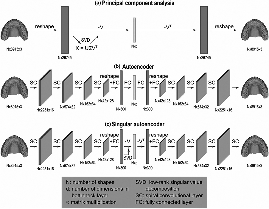
Model architecture for (A) principal component analysis, (B) an autoencoder network, and (C) a singular autoencoder network. Each model compresses 3D dental scans to a lower dimensional space of d dimensions. The principal component model is based on a low-rank singular value decomposition applied to a reshaped representation of the 3D shape data. Reconstruction of the original shape data is obtained by the inverse operation. The encoder of the autoencoder network consists of four spiral convolutional layers, followed by two fully connected layers. The decoder architecture is mirrored to the encoder architecture. The encoder of the singular autoencoder contains four spiral convolutional layers followed by one fully connected layer and a low-rank singular value decomposition. The decoder is symmetric to the encoder

2.2.2 ∣. Autoencoder

Autoencoders (AEs), like PCA, aimed to encode data into a relatively small number of scores and then reconstruct the original data from that representation. An AE consists of two main parts: the encoder that performs the compression of the data, and the decoder, that reconstructs the original data given in the output of the encoder. Typically, the decoder has a symmetric structure to the encoder, though this is not required. The shapes in our data set are represented as three-dimensional, triangulated surface meshes. This is a fundamentally different representation to the 2D and 3D volumetric images on which CNNs were first developed. To generalize the approaches to 3D mesh data, we draw on techniques of ‘geometric deep learning’.²²

Figure 2B shows the structure of the autoencoder network. The first four layers of the encoder are spiral convolutional layers in which the size of the image (number of points) is reduced. Each spiral convolutional layer consists of a spiral convolution operator followed by an exponential linear unit activation and a mesh simplification step. Spiral convolutions^23,24 are filters that are applied to each point of the image and extract important features analogous to the grid-based convolutional operators in traditional CNNs. The filters are designed as spirals starting at a centre point and proceeding outwards from a random adjacent point, in a spiral (Figure 3A). The mesh simplification step reduces the image size according to a fixed mesh simplification scheme estimated prior to building the network. The simplification scheme (Figure 3B) was defined by performing four iterations of quadric edge collapse on the template in MeshLab software.²⁵ The four spiral convolutional layers consist of 16, 32, 64, and 128 learned filters, respectively. Afterwards, two fully connected layers are added to compress the data even further to the desired number of scores. As usual, the decoder is symmetric to the encoder and, thus, consist of two fully connected layers, followed by four spiral convolutional layers. The encoder and decoder were trained simultaneously by submitting shapes of the training set to the network, computing the reconstruction error, and updating the network using the backpropagation algorithm.²⁶

FIGURE 3.

A, Example of the construction of a spiral filter. B, Four consecutive mesh simplification steps, ranging from a mesh consisting of 8915 points to a mesh comprising 42 points

2.2.3 ∣. Singular autoencoder

In this work, we propose the singular autoencoder (SAE) in which we combine the simplicity of the past (PCA) with the power of the present (AE). The aim was to preserve important properties of PCA, that is, the uncorrelatedness of the resulting scores and optimal distribution of variance across dimensions, with the extra power of AEs that can model non-linearity and can be optimized to perform additional tasks. The SAE (Figure 2C) has the same structure as the AE introduced in the previous section, except for the last layer of the encoder and the first layer of the decoder, which are replaced by a low-rank singular value decomposition²⁷ to ensure decorrelated scores.

2.3 ∣. Evaluation metrics

The models were submitted to a set of standard evaluation metrics for SSMs²⁸: (i) accuracy, which represents the models’ ability to correctly reconstruct training samples after compression; (ii) generalization, which represents the model's ability to correctly reconstruct unseen test samples; and (iii) specificity, which represents the model's ability to generate realistic new shapes. Additionally, we investigated the orthogonality of the constructed spaces. To preserve interpretability of each metric, prior to calculating the shape differences shapes were scaled back to the mean size of all dental casts.

2.3.1 ∣. Accuracy

The accuracy is defined as the mean absolute error (MAE) or the absolute difference between corresponding points of the original input shape x_i and the reconstructed output shape x′_i, averaged over all training samples:

$$A=\frac{1}{N_{train}}\sum _{i=1}^{N_{train}}\mid x_i-x_i^{\prime }\mid ,\forall x_i\in trainset$$

The accuracy of a model describes its compression power, or, in other words, its ability to efficiently capture shape variation in a compact representation for a given number of dimensions.

2.3.2 ∣. Generalization

The generalization is especially important when the model will be applied to new data sets in addition to the original training set, since it describes the model's capability to capture shape variance in unseen, or non-training, data. It is computed as the MAE for all shapes from the test set:

$$G=\frac{1}{N_{test}}\sum _{i=1}^{N_{test}}\mid x_i-x_i^{\prime }\mid ,\forall x_i\in testset$$

2.3.3 ∣. Specificity

The specificity of a model was evaluated by generating a large number N_spec (= 10000) of random synthetic shapes and validating whether they are realistic. Since realistic shapes are expected to be similar to existing shapes, the specificity is defined as the MAE between the generated shapes and their most similar shape from the training data:

$$S=\frac{1}{N_{spec}}\sum _{i=1}^{N_{spec}}\mid x_i^m-x_i^{\prime }\mid ,$$

Where x_i^m represents the most similar shape from the training data to the generated shape x′_i:

$$x_i^m\leftarrow \underset{x_j\in \text{train set}}{\text{argmin}}\mid x_j-x_i^{\prime }\mid$$

Synthetic shapes were generated by randomly sampling and reconstructing from the lower dimensional space. Samples were drawn from a multivariate normal distribution specified by the mean and covariance matrix of the scores.

In addition to the specificity, we assessed the variance of the synthetic samples as the average Euclidean distance between each of the synthetic samples and the average shape $\overline{x}$:

$$V=\frac{1}{N_{spec}}\sum _{i=1}^{N_{spec}}\mid \overline{x}-x_i^{\prime }\mid .$$

2.3.4 ∣. Uncorrelatedness of the scores

An important attribute of PCA is that the resulting scores are uncorrelated. This is useful in multivariate statistics since it guarantees an invertible covariance matrix, which is essential to many statistical operations. In active shape models it means that the fitted shape can be varied along each dimension of shape variation independently. We assessed this by plotting the covariance matrix of the scores. If scores are uncorrelated, the off-diagonal elements of the covariation matrix are zero. Additionally, we assessed the invertibility of the covariance matrix by calculating its determinant. A determinant equal to zero indicates that the inverse does not exist. To exclude differences in variance of the scores produced by different methods, we calculated the determinant of the column-normalized covariance matrix, that is, the correlation matrix.

2.4 ∣. Experiments

We compared the three models at different dimensionalities by computing the evaluation metrics, retaining different numbers of scores describing the shape of each individual cast. Each model type was trained to generate 176 scores. Starting from the initial 176 scores, the dimensions with the smallest amount of variance were dropped one by one by setting the scores along those dimensions to zero before reconstructing or synthesizing the shape. For the AE and the SAE this performance may not be the same as if the model was trained for a smaller dimensionality explicitly. Training these networks for each dimensionality explicitly is too expensive so we performed point-checks at dimensionality 50, 94 and 176. These corresponded to an explained variance of 90%, 95% and 98% in the PCA model, respectively.

3 ∣. RESULTS

3.1 ∣. Model evaluation metrics

Figure 4 shows the evaluation metrics for each model type for dimensionality ranging from 1-176. Markers indicate the evaluation metric calculated when the model was trained explicitly at that dimensionality. Table 1 shows the values corresponding to these markers and Supplementary Material. 3 plots the results for individual samples. SAE shows equal performance to PCA on all metrics and better performance compared to the AE. PCA always explains the most linear variation possible for a given number of dimensions. Therefore, its accuracy typically reflects good base performance for other models to be compared to. Equivalent accuracy between SAE and PCA indicates that SAE can compress variation into a small number of variables with equal efficiency. Equivalent generalization indicates that SAE learns important variation, as opposed to noise, with equal efficiency. Furthermore, the generalization error is approximately equal to the accuracy, indicating that the models are not overfitted. Equivalent specificity indicates that SAE and PCA generate equally realistic shapes that can be encountered in real life, while equivalent variance indicates that SAE parameterizes the range of normal shape variation as accurately as PCA. A statistical comparison of the different models is provided in Supplementary Material. 4.

FIGURE 4.

Mean accuracy, generalization, specificity and variance for a diminishing number of dimensions taken into account. The dots indicate the performance for models that are optimized to compress the data to that number of dimensions (d = 176, d = 94, and d = 50) specifically. This performance is approximately the same for all model types

TABLE 1.

Results for the accuracy, generalization, specificity, variance (mean ± standard deviation) and determinant of the correlation matrix for three different model types

		Accuracy [MM]	Generalization [MM]	Specificity [MM]	Variance [MM]	Determinant
50 dims.	PCA	226E-01 ± 533E-02	242E-01 ± 768E-02	552E-01 ± 601E-02	7,03E-01 ± 1,51E-01	1000E+00
	AE	220E-01 ± 559E-02	240E-01 ± 815E-02	544E-01 ± 595E-02	6,94E-01 ± 151E-01	2970E-07
	SAE	224E-01 ± 603E-02	2,40E-01 ± 8,21E-02	544E-01 ± 598E-02	696E-01 ± 153E-01	9995E-01
94 dims.	PCA	162E-01 ± 335E-02	179E-01 ± 587E-02	580E-01 ± 595E-02	727E-01 ± 150E-01	1000E+00
	AE	159E-01 ± 382E-02	179E-01 ± 610E-02	571E-01 ± 587E-02	719E-01 ± 148E-01	1,124E-17
	SAE	161E-01 ± 393E-02	179E-01 ± 14E-02	571E-01 ± 571E-02	717E-01 ± 145E-01	9998E-01
176 dims.	PCA	104E-01 ± 177E-02	122E-01 ± 424E-02	595E-01 ± 574E-02	740E-01 ± 147E-01	1000E+00
	AE	110E-01 ± 244E-02	130E-01 ± 469E-02	588E-01 ± 569E-02	733E-01 ± 147E-01	1426E-99
	SAE	104E-01 ± 230E-02	124E-01 ± 451E-02	589E-01 ± 568E-02	734E-01 ± 144E-01	1000E+00

Note: For each type of model, three models with different amounts of compression are constructed and evaluated. The constructed lower dimensional spaces consist of 50, 94 or 176 dimensions (dims.).

3.2 ∣. Uncorrelatedness of the scores

The covariance matrix of the 50-dimensional embedding space for each type of model is shown in Figure 5. It is observed that the covariance matrices for the PCA and SAE models show very similar behaviour, displaying large values on the diagonal and values that are zero elsewhere. Furthermore, the variance, which we find on the diagonal, is distributed over the different dimensions in such a way that for any given number of dimensions, the explained amount of variance is maximized. On the other hand, the covariance matrix for the AE model is less structured. While the largest values are still situated on the diagonal, there is also a lot of correlation between different dimensions. Moreover, the amount of variance present in each dimension is distributed more evenly over the dimensions. This is supported by the shape variance explained by the dimension with the largest variance, as depicted in Figure 1. This figure illustrates that both the PCA and SAE models can capture a lot of shape variation in a single dimension.

FIGURE 5.

Covariance matrix of the scores for the 50-dimensional spaces constructed by the different types of models. The off-diagonal elements of the covariance matrix display the correlation between the scores along different dimensions. The elements on the diagonal show the amount of variance captured by each of the dimensions. Dark (blue) values indicate low (co)variance and light (yellow) values indicate high (co)variance

4 ∣. DISCUSSION

SSMs are a useful tool in biological shape analysis as they allow for a comprehensive yet computationally efficient comparison of complex shapes. Effective SSMs are expected to generate compact representations that efficiently capture shape variation. Two common approaches are PCA and AEs. PCA is a traditional approach that compactly parameterizes normal variation on independent dimensions. AEs lie in the field of deep learning, offering non-linearity and adaptability. In this study, we introduce a novel model type, the SAE, which aims to combine the most important properties of PCA and AEs.

Results show that the SAE achieves competitive performance in terms of accuracy, generalization, specificity, and variance. This indicates that the SAE captures normal variation as accurately as PCA and AEs. An important finding was that there are no significant differences in generalization power between different models. In this instance, this means that neural network-based models, which are typically data-hungry and prone to overfitting, handle unseen data equally well as PCA, which is known to be applicable to smaller data sets. With the rise of large-scale 3D databases, this opens the possibility to construct publicly available models which can be used to score unseen data samples.

PCA generates uncorrelated scores that code variation on independent aspects of shape variation. This ability to represent shape variation as uncorrelated scores supports statistical comparisons of groups (eg sexual dimorphism in palatal shape) in two ways: firstly, uncorrelated variables ensure an invertible covariance matrix, essential to many statistical tests; secondly, scores along independent dimensions can be manipulated separately, which provides stability for active shape models.¹⁴ Moreover, PCA maximizes the variation explained for any given number of dimensions. This offers the ability to generate a large model and subsequently reduce the number of dimensions, which can help in defining a suitable dimensionality and eliminates the need to retrain smaller models. These properties of PCA are not present in regular AE networks, where there is correlation between scores on different dimensions and scores on each dimension represent a relatively small amount of shape variance. As a consequence, training for a specific dimensionality is warranted for the AE. This is disadvantageous since pre-defining the required dimensionality is a challenging and ad hoc task which heavily depends on the intended application. Even though multiple techniques to find the optimal dimensionality exist, they often rely on the ordered eigenvalues produced by PCA and are not applicable to regular AEs. Well-known techniques are, for example Horn's parallel analysis,²⁹ Kaiser criterion,³⁰ a scree plot,³¹ or retaining a certain percentage of variance explained. The last technique was used to get an initial dimensionality approximation for the different models in this work. Furthermore, the determinant of the covariance matrix for the AE is close to zero, indicating that the inverse does not exist or is unstable. In contrast to the AE, our SAE model represents shape variation as compactly as PCA on uncorrelated dimensions.

The main value of neural networks for shape analysis lies in the fact that they can model non-linearity and offer a lot of flexibility to adapt the model. While the assumption of linearity in PCA does not have a significant impact in this study, it may limit performance for more diverse data sets or for problems that are known to have a non-linear nature, such as the modelling of growth trajectories.^18,32 Furthermore, neural networks can be extended to perform additional or more complex tasks. For instance, models can be trained to optimize the lower dimensional space for classification problems, or conditional variables, such as sex and age, can be incorporated to impose more biological relevance onto the structure of the space. Moreover, they can be adapted to accept other types of input data. The networks in this work are constructed to benefit from the fact that all shapes are represented by the same mesh structure. As a result, all models in this work depend heavily on the success of the data pre-processing and none of them are able to handle dental scans without full permanent dentition. However, alternative convolutional operators exist that are designed to accept non-uniform input data. Therefore, geometric deep-learning techniques not needing this homology, for example, PointNet++,³³ are more promising towards the future for larger data sets with missing data and teeth, or data sets comprising different stages of dentition. This is an important advantage of the neural network-based models over PCA, which is inherently dependent on the homologous representation of data.

5 ∣. CONCLUSIONS

This study introduced new concepts from AI and deep learning into the context of biological shape analysis and active shape models on 3D dental casts. We introduced the SAE, a novel approach which combines important properties from traditional PCA with techniques from deep learning, that is, AE networks. An SAE model was subjected to a set of evaluation metrics to assess its ability to compress and reconstruct seen and unseen data samples and to generate new, synthetic shapes. Results confirm that the SAE reaches comparable performance to traditional approaches and combines the most important properties of both PCA and AE networks, and thus might be a useful tool for shape analysis in the future. This study was limited to shapes that underwent an elaborate pre-processing pipeline; further research might explore the possibility to adapt the neural networks to accept unprocessed data. Moreover, further work can be aimed at the construction of publicly available models, which can be used to score smaller data sets.

DATA AVAILABILITY STATEMENT

The data that support the findings of this study were collected in the context of the Pittsburgh Orofacial Cleft (POFC) study and are not publicly available at this time. Code for constructing and using models, and resulting models are available at https://gitlab.kuleuven.be/u0123700/singular_autoencoder. Other underlying code for the data pre-processing is available as part of MATLAB software, available through MathWorks (https://www.mathworks.com), and from https://github.com/TheWebMonks/meshmonk.

REFERENCES

- 1.Lione R, Franchi L, Huanca Ghislanzoni LT, Primozic J, Buongiorno M, Cozza P. Palatal surface and volume in mouth-breathing subjects evaluated with three-dimensional analysis of digital dental casts—a controlled study. Eur J Orthod. 2015;37(1):101–104. [DOI] [PubMed] [Google Scholar]
- 2.Saadeh ME, Haddad RV, Ghafari JG. Morphometric analysis of palatal rugae in different malocclusions. J Orofac Orthop. 2021;82(2):111–120. [DOI] [PubMed] [Google Scholar]
- 3.Parcha E, Bitsanis E, Halazonetis DJ. Morphometric covariation between palatal shape and skeletal pattern in children and adolescents: a cross-sectional study. Eur J Orthod. 2017;39(4):377–385. 10.1093/ejo/cjw063 [DOI] [PubMed] [Google Scholar]
- 4.Paoloni V, Lione R, Farisco F, Halazonetis DJ, Franchi L, Cozza P. Morphometric covariation between palatal shape and skeletal pattern in Class II growing subjects. Eur J Orthod. 2017;39(4):371–376. 10.1093/ejo/cjx014 [DOI] [PubMed] [Google Scholar]
- 5.Heiser W, Niederwanger A, Bancher B, Bittermann G, Neunteufel N, Kulmer S. Three-dimensional dental arch and palatal form changes after extraction and nonextraction treatment. Part 1. Arch length and area. Am J Orthod Dentofacial Orthop. 2004;126(1):71–81. 10.1016/j.ajodo.2003.05.015 [DOI] [PubMed] [Google Scholar]
- 6.Krneta B, Zhurov A, Richmond S, Ovsenik M. Diagnosis of Class III malocclusion in 7- to 8-year-old children—a 3D evaluation. Eur J Orthod. 2015;37(4):379–385. [DOI] [PubMed] [Google Scholar]
- 7.Primožič J, Ovsenik M, Richmond S, Kau CH, Zhurov A. Early crossbite correction: a three-dimensional evaluation. Eur J Orthod. 2009;31(4):352–356. [DOI] [PubMed] [Google Scholar]
- 8.Matsuyama Y, Motoyoshi M, Tsurumachi N, Shimizu N. Effects of palate depth, modified arm shape, and anchor screw on rapid maxillary expansion: a finite element analysis. Eur J Orthod. 2015;37(2):188–193. 10.1093/ejo/cju033 [DOI] [PubMed] [Google Scholar]
- 9.Ambellan F, Lamecker H, von Tycowicz C, Zachow S. Statistical shape models: understanding and mastering variation in anatomy. In: Rea PM, ed. Biomedical Visualisation. Vol 1156. Advances in Experimental Medicine and Biology. Springer International Publishing; 2019:67–84. 10.1007/978-3-030-19385-0_5 [DOI] [PubMed] [Google Scholar]
- 10.Gielis WP, Weinans H, Welsing PMJ, et al. An automated work-flow based on hip shape improves personalized risk prediction for hip osteoarthritis in the CHECK study. Osteoarthritis Cartilage. 2020;28(1):62–70. 10.1016/j.joca.2019.09.005 [DOI] [PubMed] [Google Scholar]
- 11.Verhaegen F, Meynen A, Matthews H, Claes P, Debeer P, Scheys L. Determination of pre-arthropathy scapular anatomy with a statistical shape model: part I—rotator cuff tear arthropathy. J Shoulder Elbow Surg. 2021;30(5):1095–1106. 10.1016/j.jse.2020.07.043 [DOI] [PubMed] [Google Scholar]
- 12.Audenaert EA, Duquesne K, De Roeck J, et al. Ischiofemoral impingement: the evolutionary cost of pelvic obstetric adaptation. J Hip Preserv Surg. Published online February 8, 2021:1–11. 10.1093/jhps/hnab004 [DOI] [PMC free article] [PubMed] [Google Scholar]
- 13.Woods C, Fernee C, Browne M, Zakrzewski S, Dickinson A. The potential of statistical shape modelling for geometric morphometric analysis of human teeth in archaeological research. PLoS One. 2017;12(12):e0186754. 10.1371/journal.pone.0186754 [DOI] [PMC free article] [PubMed] [Google Scholar]
- 14.Buchaillard S, Ong S, Payan Y, Foong K. 3D statistical models for tooth surface reconstruction. Comput Biol Med. 2007;37:1461–1471. 10.1016/j.compbiomed.2007.01.003 [DOI] [PubMed] [Google Scholar]
- 15.Nielsen MA. Neural networks and deep learning. Published online 2015. Accessed May 10, 2021. http://neuralnetworksanddeeplearning.com
- 16.Zhou D-X. Universality of deep convolutional neural networks. Appl Comput Harmon Anal. 2020;48(2):787–794. 10.1016/j.acha.2019.06.004 [DOI] [Google Scholar]
- 17.Hinton GE. Reducing the dimensionality of data with neural networks. Science. 2006;313(5786):504–507. 10.1126/science.1127647 [DOI] [PubMed] [Google Scholar]
- 18.Eslami Amirabadi G, Golshah A, Derakhshan S, Khandan S, Saeidipour M, Nikkerdar N. Palatal dimensions at different stages of dentition in 5 to 18-year-old Iranian children and adolescent with normal occlusion. BMC Oral Health. 2018;18(1):87. 10.1186/s12903-018-0538-y [DOI] [PMC free article] [PubMed] [Google Scholar]
- 19.White JD, Ortega-Castrillón A, Matthews H, et al. MeshMonk: open-source large-scale intensive 3D phenotyping. Sci Rep. 2019;9(1):1–11. 10.1038/s41598-019-42533-y [DOI] [PMC free article] [PubMed] [Google Scholar]
- 20.Claes P, Walters M, Clement J. Improved facial outcome assessment using a 3D anthropometric mask. Int J Oral Maxillofac Surg. 2012;41(3):324–330. 10.1016/j.ijom.2011.10.019 [DOI] [PubMed] [Google Scholar]
- 21.Blanz V, Vetter T. A Morphable Model for the Synthesis of 3D Faces. In: Proceedings of the 26th Annual Conference on Computer Graphics and Interactive Techniques -SIGGRAPH ’99. ACM Press; 1999:187–194. 10.1145/311535.311556 [DOI] [Google Scholar]
- 22.Bronstein MM, Bruna J, LeCun Y, Szlam A, Vandergheynst P. Geometric deep learning: going beyond Euclidean data. IEEE Signal Process Mag. 2017;34(4):18–42. 10.1109/MSP.2017.2693418 [DOI] [Google Scholar]
- 23.Lim I, Dielen A, Campen M, Kobbelt L. A Simple Approach to Intrinsic Correspondence Learning on Unstructured 3D Meshes. In: Proceedings of the European Conference on Computer Vision (ECCV). Springer; 2018:349–362. 10.1007/978-3-030-11015-4_26 [DOI] [Google Scholar]
- 24.Gong S, Chen L, Bronstein M, Zafeiriou S. SpiralNet++: A Fast and Highly Efficient Mesh Convolution Operator. In: 2019 IEEE/CVF International Conference on Computer Vision Workshop (ICCVW). IEEE; 2019:4141–4148. 10.1109/ICCVW.2019.00509 [DOI] [Google Scholar]
- 25.Cignoni P, Callieri M, Corsini M, Dellepiane M, Ganovelli F, Ranzuglia G. MeshLab: an open-source mesh processing tool. In: Scarano V, Chiara RD, Erra U, eds. Eurographics Italian Chapter Conference. The Eurographics Association; 2008. 10.2312/LocalChapterEvents/ItalChap/ItalianChapConf2008/129-136 [DOI] [Google Scholar]
- 26.Kelley HJ. Gradient theory of optimal flight paths. Ars Journal. 1960;30(10):947–954. [Google Scholar]
- 27.Halko N, Martinsson PG, Tropp JA. Finding structure with randomness: probabilistic algorithms for constructing approximate matrix decompositions. SIAM Rev. 2011;53(2):217–288. 10.1137/090771806 [DOI] [Google Scholar]
- 28.Audenaert E, Pattyn C, Steenackers G, De J, Vandermeulen D, Claes P. Statistical shape modelling of skeletal anatomy for sex discrimination: their training size, sexual dimorphism and asymmetry. Front Bioeng Biotechnol. 2019;7:302. [DOI] [PMC free article] [PubMed] [Google Scholar]
- 29.Horn JL. A rationale and test for the number of factors in factor analysis. Psychometrika. 1965;30:179–185. 10.1007/BF02289447 [DOI] [PubMed] [Google Scholar]
- 30.Kaiser HF. The application of electronic computers to factor analysis. Educ Psychol Meas. 1960;20(1):141–151. 10.1177/001316446002000116 [DOI] [Google Scholar]
- 31.Cattell RB. The scree test for the number of factors. Multivariate Behav Res. 1966;1(2):245–276. 10.1207/s15327906mbr0102_10 [DOI] [PubMed] [Google Scholar]
- 32.Matthews HS, Penington AJ, Hardiman R, et al. Modelling 3D craniofacial growth trajectories for population comparison and classification illustrated using sex-differences. Sci Rep. 2018;8(1):1–11. 10.1038/s41598-018-22752-5 [DOI] [PMC free article] [PubMed] [Google Scholar]
- 33.Ge L, Cai Y, Weng J, Yuan J. Hand PointNet: 3D Hand Pose Estimation Using Point Sets. IEEE/CVF Conference on Computer Vision and Pattern Recognition; 2018:8417–8426. 10.1109/CVPR.2018.00878 [DOI] [Google Scholar]
Associated Data
This section collects any data citations, data availability statements, or supplementary materials included in this article.
Supplementary Materials