Abstract
Climate changes are top biodiversity shapers, both during the past and future. Mapping the most climatic stable and unstable zones on Earth could improve our understanding of biodiversity distribution and evolution. Here, we present a set of maps based on a global scale, high resolution (ca. 5 km) new Climate Stability Index (CSI). The CSI considers bioclimatic variables for two different time ranges: (1) from Pliocene (3.3 Ma) to the present (CSI-past map set), using 12 time periods of PaleoClim representing warm and cold cycles; and (2) from present to the year 2100 (CSI-future), using nine general circulation models of climate change of four periods available from WorldClim. We calculated standard deviation of the variables and selected an uncorrelated set for summing, normalizing and obtaining the CSI maps. Our approach is useful for fields such as biogeography, earth sciences, agriculture, or sociology. However, CSI is an index that can be re-calculated according to particular criteria and objectives (e.g. temperature variables); maps are, therefore, customizable to every user.
Subject terms: Projection and prediction, Biogeography
| Measurement(s) | climate stability index |
| Technology Type(s) | general circulation models of climate change |
| Factor Type(s) | temporal interval |
| Sample Characteristic - Environment | climate system • climate change |
| Sample Characteristic - Location | global |
Machine-accessible metadata file describing the reported data: 10.6084/m9.figshare.19050569
Background & Summary
Long-term climatic variation has had an enormous impact on the evolution of biodiversity, including humans. Climatic instability linked to the Pleistocene glacial/interglacial cycles has caused active diversification1–3. In contrast, regions with relatively stable climates have often acted either as “museums” (places of persistence)4,5 or both as “museums” and “cradles”6,7. In addition, recent global warming is causing even deeper changes in biodiversity in a very short space of time. Increases of temperature in just a few decades might produce large regional species turnover by increasing extinction rates and large migrations8, and also by loss of phylogenetic diversity (= evolutionary potential)9.
Identifying areas with high climatic stability is of enormous interest. Delimiting past trends of stability and mapping them can help to shed light into evolutionary processes that shaped current biota, including human evolution. They may also be helpful in designing new protected areas (PAs) and prioritizing or redesigning the existing ones10, following the demand of incorporating evolutionary processes into conservation planning11. Mapping climatic stability for the future can be even more important, as climate patterns are predicted to change dramatically during this century, including the occurrence of extreme weather events8,12. Such mapping may have, thus, implications on economy and human health; e.g., when selecting new arable lands or new human settlements that will be needed as a consequence of the predicted large-scale migrations8.
Attempts to cartography climate stability are not new. The only ones that offer data at a global scale are StableClim13 and the “map of climate stability”14 (hereinafter “MCS”), which are projections of climate variation, the former from 21,000 BP (LGM or Last Glacial Maximum) to 2100 CE13, and the latter from 21,000 BP to 100 BP14. StableClim offers estimates of climate stability on an ideal time-scale (every 100 years) for surveying the eco-evolutionary impacts of short-term climate shifts13, but it shares with MCS three limitations14: (1) coverage of only ca. 21,000 years, which hinders their utility for explaining the role of climate stability in evolution and speciation that take thousands or millions of years; (2) spatial resolution is insufficient (2.5° grid, ca. 278 km at the equator), which does not allow one to correlate climatic stability with population data on both local and regional scales; and (3) they use one or two variables (mean monthly temperatures13 or mean monthly temperatures and precipitations14) that may not be the key ones for a given case of study; for example, distribution patterns of bees in South Africa are highly dependent on seasonality and not on mean rainfall values15.
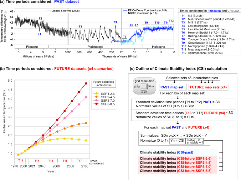
Thanks to the recent publication of PaleoClim16, a free-access database of paleoclimate layers at 2.5 arc-min (~5 km) grid resolution that includes data much older than the LGM, we are presenting a new set of maps that are based on a new Climatic Stability Index (CSI). Given the markedly different speed of inferred climatic changes (see above), we divide the sets of maps into two: CSI-past and CSI-future. CSI-past is based on the 12 time periods (listed in Fig. 1a) included in PaleoClim16, which span from 3.3 Ma (Pliocene) to present. CSI-future uses the average values of nine general circulation models (GCMs) along four time intervals until 2100 (Fig. 1b), available in WorldClim17. CSI-future offers maps of climate stability for four Shared Socioeconomic Pathways (SSP18; Fig. 1b) that will be used to produce the IPCC Sixth Assessment Report on climate change. Variables for CSI calculation (Table 1) include annual averages (e.g. annual mean temperature), extremes (e.g. minimum temperature of coldest month), and seasonality (e.g. annual range in temperatures). CSI-past takes into account 14 bioclimatic variables, while CSI-future uses five more.
Fig. 1.
General overview of time periods considered to calculate the Climate Stability Index (CSI) for past and future map sets and graphical illustration of index generation. (a) Time periods used to estimate the CSI-past and from which paleoclimate data have been taken (from PaleoClim16 database, which includes two map sets from CHELSA25), represented by a Pliocene to Holocene temperature reconstruction modified from https://en.wikipedia.org/wiki/Geologic_temperature_record. Temperature reconstruction showed in a black line derived from Lisiecki and Raymo26. (b) Time periods and four Shared Socioeconomic Pathways (SSPs: SSP1-2.6, SSP2-4.5, SSP3-7.0, and SSP5-8.5) considered to estimate CSI-future using climate data from WorldClim17, modified from Gidden et al.27. (c) Schematic representation of the methodology employed to calculate the CSI for each map set.
Table 1.
Bioclimatic variables used to generate the Climate Stability Index (CSI) maps.
| Variable | Unit | Map set (source) | Included in CSI maps |
|---|---|---|---|
| Bio1: Annual mean temperature | °C | Past (PaleoClim) | Past |
| Future (WorldClim v2) | Future (SSP3) | ||
| Bio2: Mean diurnal range (Mean of monthly (max. temp. - min. temp.)) | °C | Future (WorldClim v2) | Future (SSP1, SSP2, SSP3, SSP5) |
| Bio3: Isothermality (bio2/bio7) (×100) | dls | Future (WorldClim v2) | Future (SSP1, SSP2, SSP3, SSP5) |
| Bio4: Temperature seasonality (standard deviation ×100) | °C | Past (PaleoClim) | Past |
| Future (WorldClim v2) | |||
| Bio5: Max. temperature of warmest month | °C | Future (WorldClim v2) | Future (SSP3) |
| Bio6: Min. temperature of coldest month | °C | Future (WorldClim v2) | Future (SSP1, SSP2) |
| Bio7: Temperature annual range (bio5-bio6) | °C | Future (WorldClim v2) | Future (SSP1, SSP5) |
| Bio8: Mean temperature of wettest quarter | °C | Past (PaleoClim) | Future (SSP1, SSP2, SSP3, SSP5) |
| Future (WorldClim v2) | |||
| Bio9: Mean temperature of driest quarter | °C | Past (PaleoClim) | Past |
| Future (WorldClim v2) | Future (SSP1, SSP2, SSP3, SSP5) | ||
| Bio10: Mean temperature of warmest quarter | °C | Past (PaleoClim) | Future (SSP1, SSP2, SSP5) |
| Future (WorldClim v2) | |||
| Bio11: Mean temperature of coldest quarter | °C | Past (PaleoClim) | Past |
| Future (WorldClim v2) | |||
| Bio12: Annual precipitation | mm | Past (PaleoClim) | Past |
| Future (WorldClim v2) | Future (SSP1, SSP3, SSP5) | ||
| Bio13: Precipitation of wettest month | mm | Past (PaleoClim) | Past |
| Future (WorldClim v2) | Future (SSP3, SSP5) | ||
| Bio14: Precipitation of driest month | mm | Past (PaleoClim) | Past |
| Future (WorldClim v2) | Future (SSP1) | ||
| Bio15: Precipitation seasonality (coefficient of variation) | dls | Past (PaleoClim) | Past |
| Future (WorldClim v2) | Future (SSP1, SSP2, SSP3, SSP5) | ||
| Bio16: Precipitation of wettest quarter | mm | Past (PaleoClim) | Future (SSP2) |
| Future (WorldClim v2) | |||
| Bio17: Precipitation of driest quarter | mm | Past (PaleoClim) | Future (SSP2, SSP3, SSP5) |
| Future (WorldClim v2) | |||
| Bio18: Precipitation of warmest quarter | mm | Past (PaleoClim) | Past |
| Future (WorldClim v2) | Future (SSP1, SSP2, SSP3, SSP5) | ||
| Bio19: Precipitation of coldest quarter | mm | Past (PaleoClim) | Past |
| Future (WorldClim v2) | Future (SSP1, SSP2, SSP3, SSP5) |
For each variable we include the following information: the units, whether they are included in a climate map set (and source from where it can be downloaded), and whether they have been taken into account to calculate the CSI. Note that bio2, bio3, bio5, bio6 and bio7 were not included for the calculation of CSI-past as these variables are not available in PaleoClim database16 for T1 (M2, Pliocene, ca. 3.3 Ma), T2 (mid-Pliocene warm period, Pliocene, 3.205 Ma), and T3 (MIS19, Pleistocene, ca. 787 ka). Unit abbreviations: °C (Celsius), mm (millimetres), dls (dimensionless).
In spite of the limitation of using only 12 time periods as a basis for inferring the long-term climatic stability (with only three older to 0.12 Ma), the much wider time interval, the variety of measures (means, peaks, and intra-year variability) and the finer resolution (ca. 5 km) makes our proposal a very versatile tool with a wide array of applications. With both CSI-past and CSI-future we offer maps of climatic stability adhering to FAIR principles19, adaptable to every user and circumstance: they are very easy to use and the variables to estimate the climate stability can be selected at the user’s discretion.
Methods
A workflow for the calculation of CSI is presented in Fig. 1c. For all the analyses, we used the R v. 4.0.3 software environment20 implemented in RStudio v. 1.4.1103. The scripts used for each methodological step are available at the Figshare repository21. After data download from primary sources (PaleoClim and WorldClim), specifically for the CSI-future map set we performed an initial step aimed to obtain individual bioclimatic variables for each future time period for the four SSPs (Fig. 1b). To achieve this, the median values of nine GCMs were calculated in functions compiled in raster R package22 for each individual bioclimatic variable (see a few exceptions of number of GCMs used in Table 2).
Table 2.
General circulation models (GCM) used to construct the future map sets.
| 2021–2040 | ||||
|---|---|---|---|---|
| GCM | SSP1-2.6 | SSP2-4.5 | SSP3-7.0 | SSP5-8.5 |
| BCC-CSM2-MR | ✓ | ✓ | ✓ | ✓ |
| CNRM-CM6-1 | ✓ | ✓ | ✓ | ✓ |
| CNRM-ESM2-1 | ✓ | ✓ | ✓ | ✓ |
| CanESM5 | ✓ | ✓ | ✓ | ✓ |
| GFDL-ESM4 | ✓ | NA | ✓ | NA |
| IPSL-CM6A-LR | ✓ | NA | ✓ | ✓ |
| MIROC-ES2L | ✓ | ✓ | ✓ | ✓ |
| MIROC6 | ✓ | ✓ | ✓ | ✓ |
| MRI-ESM2-0 | ✓ | ✓ | ✓ | NA |
| 2041–2060 | ||||
| GCM | SSP1-2.6 | SSP2-4.5 | SSP3-7.0 | SSP5-8.5 |
| BCC-CSM2-MR | ✓ | ✓ | ✓ | ✓ |
| CNRM-CM6-1 | ✓ | ✓ | ✓ | ✓ |
| CNRM-ESM2-1 | ✓ | ✓ | ✓ | ✓ |
| CanESM5 | ✓ | ✓ | ✓ | ✓ |
| GFDL-ESM4 | ✓ | NA | ✓ | NA |
| IPSL-CM6A-LR | ✓ | ✓ | ✓ | ✓ |
| MIROC-ES2L | ✓ | ✓ | ✓ | ✓ |
| MIROC6 | ✓ | ✓ | ✓ | ✓ |
| MRI-ESM2-0 | ✓ | ✓ | ✓ | ✓ |
| 2061–2080 | ||||
| GCM | SSP1-2.6 | SSP2-4.5 | SSP3-7.0 | SSP5-8.5 |
| BCC-CSM2-MR | ✓ | ✓ | ✓ | ✓ |
| CNRM-CM6-1 | ✓ | ✓ | ✓ | ✓ |
| CNRM-ESM2-1 | ✓ | ✓ | ✓ | ✓ |
| CanESM5 | ✓ | ✓ | ✓ | ✓ |
| GFDL-ESM4 | ✓ | NA | ✓ | NA |
| IPSL-CM6A-LR | ✓ | ✓ | ✓ | ✓ |
| MIROC-ES2L | ✓ | ✓ | ✓ | ✓ |
| MIROC6 | ✓ | ✓ | ✓ | ✓ |
| MRI-ESM2-0 | ✓ | ✓ | ✓ | ✓ |
| 2081–2100 | ||||
| GCM | SSP1-2.6 | SSP2-4.5 | SSP3-7.0 | SSP5-8.5 |
| BCC-CSM2-MR | ✓ | ✓ | ✓ | ✓ |
| CNRM-CM6-1 | ✓ | ✓ | ✓ | ✓ |
| CNRM-ESM2-1 | ✓ | ✓ | ✓ | ✓ |
| CanESM5 | ✓ | ✓ | ✓ | ✓ |
| GFDL-ESM4 | ✓ | NA | ✓ | NA |
| IPSL-CM6A-LR | ✓ | ✓ | ✓ | ✓ |
| MIROC-ES2L | ✓ | ✓ | ✓ | ✓ |
| MIROC6 | ✓ | ✓ | ✓ | ✓ |
| MRI-ESM2-0 | ✓ | ✓ | ✓ | ✓ |
Those GCM marked with “NA” correspond to non-available models in WorldClim17 database, and thus not used for the calculation of means and medians.
The standard deviation (SD) was estimated as a measure of the amount of variation or dispersion along time series, from which the resulting output maps showed the places where climate conditions remained constant or variable across the temporal periods considered (Fig. 1a,b). The SD, as a way to identify stable/unstable climatic areas, was previously used in other climatic or evolutionary studies4,14. To compute the SD output rasters, we applied the mosaic function setting “fun = sd” from raster R package, calculating the SD for each pixel in the 12 time period rasters for CSI-past and five times for CSI-future, independently for each variable. The mosaic function was also used for the range calculation, with “fun = min” and “fun = max” to obtain the minimum and maximum values of input rasters, respectively, with a further step for subtracting maximum to minimum values.
Specifically, for CSI-past, as it includes several time periods with sea-level dropping below the present level (T1, T3, T5, T6, T7, T8, T9; Fig. 1a), we applied a mask of the current land surface, i.e. taking the T12 (Anthropocene) as a template. With this additional step, we were able to remove those pixels (grid cells) currently under the sea but that were once emerged. Most of these pixels, however, were only emerged during the LGM (ca. 21 ka), thus having values for bioclimatic variables for just a single time period (instead of the 12 routinely used for the variability estimation). The inclusion of these areas would result in highly climatically stable regions (low SD values; Supplementary Fig. 1), but this would be an obviously biased result. In contrast, we did not remove those areas affected by the sea-level rising periods, as only three periods contained “NoData” values (T2, T4, T10; Fig. 1a). However, to take this fact into consideration, we created a raster file in which these areas submerged during warm periods are indicated (see Supplementary Fig. 1). Finally, for both CSI-past and CSI-future, the resulting SD values were normalized to values between 0 and 1, with 0 representing completely stable areas and 1 the most unstable ones.
The next step was focused on the selection of a relatively uncorrelated set of variables for each map set. We used the removeCollinearity function from virtualspecies R package23 that estimates the correlation value among pairs of variables from a given number of random sample points (10,000 in present case) according to a given method (Pearson for the present case) and a threshold of statistic selected (r > 0.8 as a cut-off value). The function removeCollinearity returns a list of uncorrelated variables according to the settings specified, randomly selecting just one variable from groups of correlated ones (see Table 1 for a complete list of variables used for each map set). As we compiled estimates of variability independently for each variable and map set (e.g. SD bio1 past, SD bio2 past, etc.), each user can define his own CSI, selecting the more interesting variables according to the case of study.
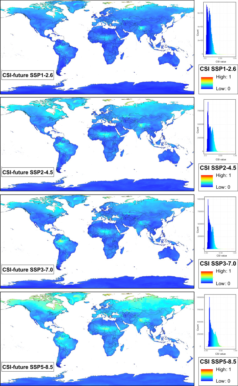
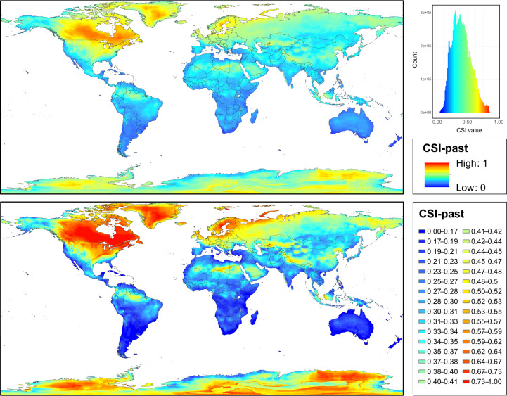
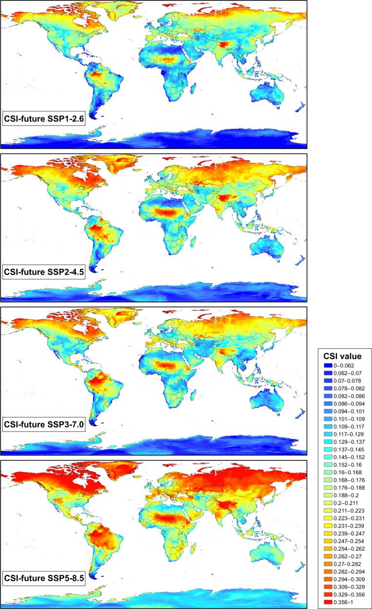
The final CSI maps were obtained by summing the SD values of the variables selected and the subsequent outputs normalized (0 to 1) (Figs. 2–4). Histogram plots were represented with ggplot2 R package24 and maps were exported with ArcGIS v.10.2.2 (Esri, Redlands, California, USA 2014). The histograms were computed for these final CSI maps, which represent the frequency and distribution of CSI values. We presented the final CSI maps with two different colour ramp schemes with ArcGIS. The first consisted of defining equal interval breaks from 0 to 1. The second was based on defining 32 categories with different value breaks for past and future map sets according to the value frequency shown by the histogram plot, i.e. the category with the highest CSI values (no. 32) was 0.71–1 in the past map set and 0.356–1 in the future map set.
Fig. 3.
Maps of Climate Stability Index (CSI) values for the future conditions (Shared Socioeconomic Pathways: SSP1-2.6, SSP2-4.5, SSP3-7.0, and SSP5-8.5) from present (1970–2000) to future (2100), at 2.5 arc-min grid resolution. Colours range from blue for low standard deviation (SD) values, which represents areas with low climatic fluctuations (i.e, low values of CSI) from present to future, to red for high SD values, which shows areas where high climatic fluctuations would have taken place (i.e., high values of CSI). The colour ramp shows equal interval breaks. The histogram with frequency and distribution of CSI values is also shown for each future scenario.
Fig. 2.
Maps of Climate Stability Index (CSI) values for the past map set from Pliocene (3.3 Ma) to present (1979–2013), at 2.5 arc-min grid resolution. Colours range from blue for low standard deviation (SD) values, which represents areas with low climatic fluctuations (i.e, low values of CSI) during the period Pliocene–present, to red for high SD values, which shows areas where high climatic fluctuations would have taken place (i.e., high values of CSI). On the upper map, the colour ramp shows equal interval breaks. The histogram with frequency and distribution of CSI values is also shown. On the lower map, the colour ramp has been manually adjusted to a defined set of break values (see details in the text).
Fig. 4.
Maps of Climate Stability Index (CSI) values for the future conditions (Shared Socioeconomic Pathways: SSP1-2.6, SSP2-4.5, SSP3-7.0, and SSP5-8.5) from present (1970–2000) to future (2100), at 2.5 arc-min grid resolution. Colours range from blue for low standard deviation (SD) values, which represents areas with low climatic fluctuations (i.e, low values of CSI) from present to future, to red for high SD values, which shows areas where high climatic fluctuations would have taken place (i.e., high values of CSI). The colour ramp has been manually adjusted to a defined set of break values (see details in the text).
Data Records
Our data records are available through Figshare21 in format of map raster layers (.TIF format).
Two sets of data records are stored:
SD-based maps of individual bioclimatic variables, which contain a set of raster layers (one for each variable): 14 for the case of the past map set (bio2, bio3, bio5, bio6, bio7 are missing) and 19 for the future map sets based on median calculations. These layers contain individual measures of the SD of each variable, which could be independently used according to the user’s study purpose or combined according to the user’s preferences to generate a customized CSI.
the five CSI-based maps presented in this study, corresponding to CSI-past, CSI-future SSP1-2.6, CSI-future SSP2-4.5, CSI-future SSP3-7.0, and CSI-future SSP5-8.5.
Data files share a common naming pattern:
For Past map set from individual variables and CSI, respectively:
“sd_past_<bioclimatic variable>.tif”
“csi_past.tif”
For Future map sets from individual variables and CSI, respectively:
“sd_future_<SSP scenario>_<bioclimatic variable>.tif”
“csi_future_<SSP scenario>.tif”
In addition, for the CSI-past map set, we include a map showing the areas affected by sea-level rising periods (intergl_affected.tif) and the raster map used to remove regions with landmasses currently under the sea but that were once emerged (lgm_del_mask.tif; see Supplementary Fig. 1).
Technical Validation
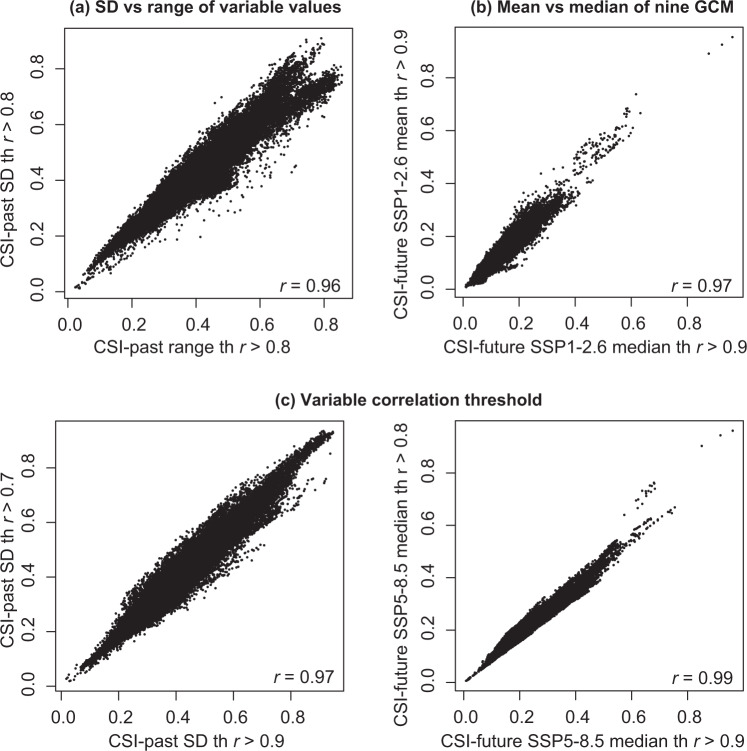
To evaluate the robustness of the CSI index, we compared its performance by varying the statistics used for its calculation (see detailed workflow in Fig. 5). For the past map set, the CSI was computed independently by means of SD and range. For the future map sets, the CSI was computed using the mean and the median of the nine GCMs to obtain individual future rasters for each time and SSPs. In parallel, the sensitivity derived from selecting a more restrictive variable correlation threshold (r > 0.7), an intermediate (r > 0.8), or a less restrictive cut-off value (r > 0.9) was also checked. In Supplementary Tables 1 and 2 the variables selected for each r threshold tested are specified. All pairs of CSI rasters were compared through Pearson’s correlation analyses, which showed a very high r value, ranging from 0.93 to 1.00. All r values in Table 3 and all correlation scatterplots are available in Supplementary Fig. 2 and some examples are included in Fig. 6. As a conclusion, methodological choices resulted in a non-remarkable impact of metric selected (mean vs. median, SD vs. range) or correlation threshold set (r > 0.7, 0.8, 0.9). Our choice was using the SD, median, and threshold r > 0.8, to draw the CSI-based maps.
Fig. 5.
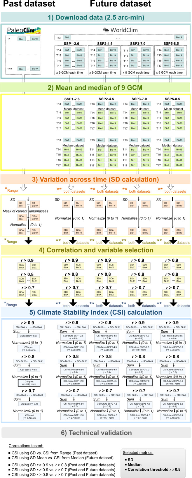
Detailed workflow of analyses employed to calculate and test the robustness of the Climate Stability Index (CSI) for past and future map sets. Final maps presented were obtained with conditions marked with wide-lined frame in the fifth step, which are: SD applying r > 0.8 threshold for variable correlation in past map set, and SD from median of nine GCM and applying r > 0.8 threshold for variable correlation in future map sets. Note that in the third step further analyses are repeated for the range statistic in the case of past map set and for both future map sets (mean and median).
Table 3.
Correlation values (Pearson’s r) of Technical Validation procedure.
| Validation category | Correlation pairs | r |
|---|---|---|
| SD vs. range | CSI-past SD th 0.7 vs. CSI-past range th 0.7 | 0.94 |
| CSI-past SD th 0.8 vs. CSI-past range th 0.8 | 0.96 | |
| CSI-past SD th 0.9 vs. CSI-past range th 0.9 | 0.97 | |
| mean vs. median | CSI-future mean SSP1-2.6 th 0.7 vs. CSI-future median SSP1-2.6 th 0.7 | 1.00 |
| CSI-future mean SSP1-2.6 th 0.8 vs. CSI-future median SSP1-2.6 th 0.8 | 1.00 | |
| CSI-future mean SSP1-2.6 th 0.9 vs. CSI-future median SSP1-2.6 th 0.9 | 0.97 | |
| CSI-future mean SSP2-4.5 th 0.7 vs. CSI-future median SSP2-4.5 th 0.7 | 1.00 | |
| CSI-future mean SSP2-4.5 th 0.8 vs. CSI-future median SSP2-4.5 th 0.8 | 1.00 | |
| CSI-future mean SSP2-4.5 th 0.9 vs. CSI-future median SSP2-4.5 th 0.9 | 1.00 | |
| CSI-future mean SSP3-7.0 th 0.7 vs. CSI-future median SSP3-7.0 th 0.7 | 1.00 | |
| CSI-future mean SSP3-7.0 th 0.8 vs. CSI-future median SSP3-7.0 th 0.8 | 1.00 | |
| CSI-future mean SSP3-7.0 th 0.9 vs. CSI-future median SSP3-7.0 th 0.9 | 1.00 | |
| CSI-future mean SSP5-8.5 th 0.7 vs. CSI-future median SSP5-8.5 th 0.7 | 1.00 | |
| CSI-future mean SSP5-8.5 th 0.8 vs. CSI-future median SSP5-8.5 th 0.8 | 1.00 | |
| CSI-future mean SSP5-8.5 th 0.9 vs. CSI-future median SSP5-8.5 th 0.9 | 1.00 | |
| threshold (r) | CSI-past SD th 0.7 vs. CSI-past SD th 0.8 | 0.95 |
| CSI-past SD th 0.7 vs. CSI-past SD th 0.9 | 0.97 | |
| CSI-past SD th 0.8 vs. CSI-past SD th 0.9 | 0.98 | |
| CSI-past range th 0.7 vs. CSI-past range th 0.8 | 0.98 | |
| CSI-past range th 0.7 vs. CSI-past range th 0.9 | 0.95 | |
| CSI-past range th 0.8 vs. CSI-past range th 0.9 | 0.99 | |
| CSI-future mean SSP1-2.6 th 0.7 vs. CSI-future mean SSP1-2.6 th 0.8 | 0.99 | |
| CSI-future mean SSP1-2.6 th 0.7 vs. CSI-future mean SSP1-2.6 th 0.9 | 0.99 | |
| CSI-future mean SSP1-2.6 th 0.8 vs. CSI-future mean SSP1-2.6 th 0.9 | 0.99 | |
| CSI-future mean SSP2-4.5 th 0.7 vs. CSI-future mean SSP2-4.5 th 0.8 | 0.96 | |
| CSI-future mean SSP2-4.5 th 0.7 vs. CSI-future mean SSP2-4.5 th 0.9 | 0.93 | |
| CSI-future mean SSP2-4.5 th 0.8 vs. CSI-future mean SSP2-4.5 th 0.9 | 0.99 | |
| CSI-future mean SSP3-7.0 th 0.7 vs. CSI-future mean SSP3-7.0 th 0.8 | 0.98 | |
| CSI-future mean SSP3-7.0 th 0.7 vs. CSI-future mean SSP3-7.0 th 0.9 | 0.99 | |
| CSI-future mean SSP3-7.0 th 0.8 vs. CSI-future mean SSP3-7.0 th 0.9 | 0.98 | |
| CSI-future mean SSP5-8.5 th 0.7 vs. CSI-future mean SSP5-8.5 th 0.8 | 0.98 | |
| CSI-future mean SSP5-8.5 th 0.7 vs. CSI-future mean SSP5-8.5 th 0.9 | 0.99 | |
| CSI-future mean SSP5-8.5 th 0.8 vs. CSI-future mean SSP5-8.5 th 0.9 | 0.99 | |
| CSI-future median SSP1-2.6 th 0.7 vs. CSI-future median SSP1-2.6 th 0.8 | 0.99 | |
| CSI-future median SSP1-2.6 th 0.7 vs. CSI-future median SSP1-2.6 th 0.9 | 0.96 | |
| CSI-future median SSP1-2.6 th 0.8 vs. CSI-future median SSP1-2.6 th 0.9 | 0.96 | |
| CSI-future median SSP2-4.5 th 0.7 vs. CSI-future median SSP2-4.5 th 0.8 | 0.96 | |
| CSI-future median SSP2-4.5 th 0.7 vs. CSI-future median SSP2-4.5 th 0.9 | 0.93 | |
| CSI-future median SSP2-4.5 th 0.8 vs. CSI-future median SSP2-4.5 th 0.9 | 0.99 | |
| CSI-future median SSP3-7.0 th 0.7 vs. CSI-future median SSP3-7.0 th 0.8 | 0.98 | |
| CSI-future median SSP3-7.0 th 0.7 vs. CSI-future median SSP3-7.0 th 0.9 | 0.99 | |
| CSI-future median SSP3-7.0 th 0.8 vs. CSI-future median SSP3-7.0 th 0.9 | 0.98 | |
| CSI-future median SSP5-8.5 th 0.7 vs. CSI-future median SSP5-8.5 th 0.8 | 0.98 | |
| CSI-future median SSP5-8.5 th 0.7 vs. CSI-future median SSP5-8.5 th 0.9 | 0.99 | |
| CSI-future median SSP5-8.5 th 0.8 vs. CSI-future median SSP5-8.5 th 0.9 | 0.99 |
Abbreviations used: SD (Standard Deviation), CSI (Climate Stability Index), th (threshold), r (r statistic of Pearson’s correlation analysis).
Fig. 6.
Pearson’s correlation coefficient (r) for examples of Climate Stability Index (CSI) pair comparisons: (a) between SD and range variable values of the past map set; (b) between mean and median of General Circulation Models of future map sets; and (c) between r > 0.7 and r > 0.9 (left) and between r > 0.8 and r > 0.9 (right) of Pearson cut-off values to remove highly correlated variables.
Before concluding, however, it should be acknowledged that the fact of not using the same approaches for past and future climate stability assessments introduces a degree of uncertainty when considered as a whole. To obtain CSI-past maps we are using PaleoClim, which provide simulations from single models for different time periods, whereas for CSI-future maps we are employing an ensemble of nine model simulations (and, thus, there is regional variability in stability).
Supplementary information
Acknowledgements
Financial support from the Ministerio de Ciencia e Innovación (projects CGL2015-66703-P MINECO/FEDER, PID2019-105583GB-C21 funded by MCIN/AEI/10.13039/501100011033, and PID2020-119163GB-I00 funded by MCIN/AEI/10.13039/501100011033; and Ph.D. grant to S.H.M from project CGL2015-66703-P) and the Catalan government (“Ajuts a grups consolidats” 2017-SGR1116). This study has been performed under the Ph.D. program “Plant Biology and Biotechnology” of the Autonomous University of Barcelona (UAB). H.O. and T.M. were funded by the Environment Research and Technology Development Fund (JPMEERF20202002) of the Environmental Restoration and Conservation Agency of Japan.
Author contributions
S.H.M., N.N. and J.L.P. designed and outlined the project, with contributions from A.S., C.Q.T., H.O., N.G.J., M.G.C. and T.M. The analyses were carried out by S.H.M., who wrote the manuscript together with J.L.P. N.N. suggested significant changes to the paper. All authors reviewed and agreed on the final submitted version of the manuscript.
Code availability
Commented R codes used to generate CSI are available at Figshare21.
Competing interests
The authors declare no competing interests.
Footnotes
Publisher’s note Springer Nature remains neutral with regard to jurisdictional claims in published maps and institutional affiliations.
Contributor Information
Sonia Herrando-Moraira, Email: sonia.herrando@gmail.com.
Jordi López-Pujol, Email: jlopez@ibb.csic.es.
Supplementary information
The online version contains supplementary material available at 10.1038/s41597-022-01144-5.
References
- 1.Rangel TF, et al. Modeling the ecology and evolution of biodiversity: Biogeographical cradles, museums, and graves. Science. 2018;361:eaar5452. doi: 10.1126/science.aar5452. [DOI] [PubMed] [Google Scholar]
- 2.Liu Y, et al. Sino‐Himalayan mountains act as cradles of diversity and immigration centres in the diversification of parrotbills (Paradoxornithidae) J. Biogeogr. 2016;43:1488–1501. doi: 10.1111/jbi.12738. [DOI] [Google Scholar]
- 3.Owen RB, et al. Progressive aridification in East Africa over the last half million years and implications for human evolution. Proc. Natl. Acad. Sci. USA. 2018;115:11174–11179. doi: 10.1073/pnas.1801357115. [DOI] [PMC free article] [PubMed] [Google Scholar]
- 4.Tang CQ, et al. Identifying long-term stable refugia for relict plant species in East Asia. Nat. Commun. 2018;9:4488. doi: 10.1038/s41467-018-06837-3. [DOI] [PMC free article] [PubMed] [Google Scholar]
- 5.Sundaram M, et al. Accumulation over evolutionary time as a major cause of biodiversity hotspots in conifers. Proc. R. Soc. B. 2019;286:20191887. doi: 10.1098/rspb.2019.1887. [DOI] [PMC free article] [PubMed] [Google Scholar]
- 6.Morales-Barbero J, Ariel Martinez P, Ferrer-Castán D, Olalla-Tárraga MA. Quaternary refugia are associated with higher speciation rates in mammalian faunas of the Western Palaearctic. Ecography. 2018;41:607–621. doi: 10.1111/ecog.02647. [DOI] [Google Scholar]
- 7.Cowling RM, et al. Variation in plant diversity in mediterranean-climate ecosystems: the role of climatic and topographical stability. J. Biogeogr. 2015;42:552–564. doi: 10.1111/jbi.12429. [DOI] [Google Scholar]
- 8.Hoegh-Guldberg, O. et al. in Global Warming of 1.5 °C. An IPCC Special Report on the Impacts of Global Warming of 1.5 °C Above Pre-industrial Levels and Related Global Greenhouse Gas Emission Pathways, in the Context of Strengthening the Global Response to the Threat of Climate Change, Sustainable Development, and Efforts to Eradicate Poverty (eds. Masson-Delmotte, V. et al.), 175–311 (Intergovernmental Panel on Climate Change, 2019).
- 9.Park DS, et al. Machine learning predicts large scale declines in native plant phylogenetic diversity. New Phytol. 2020;227:1544–1556. doi: 10.1111/nph.16621. [DOI] [PubMed] [Google Scholar]
- 10.Iwamura T, Wilson KA, Venter O, Possingham HP. A climatic stability approach to prioritizing global conservation investments. PLoS ONE. 2010;5:e15103. doi: 10.1371/journal.pone.0015103. [DOI] [PMC free article] [PubMed] [Google Scholar]
- 11.Klein C, et al. Incorporating ecological and evolutionary processes into continental-scale conservation planning. Ecol. Appl. 2009;19:206–217. doi: 10.1890/07-1684.1. [DOI] [PubMed] [Google Scholar]
- 12.Brown SC, Wigley TML, Otto-Bliesner BL, Rahbek C, Fordham DA. Persistent Quaternary climate refugia are hospices for biodiversity in the Anthropocene. Nat. Clim. Change. 2020;10:244–248. doi: 10.1038/s41558-019-0682-7. [DOI] [Google Scholar]
- 13.Brown SC, Wigley TML, Otto-Bliesner BL, Fordham DA. StableClim, continuous projections of climate stability from 21000 BP to 2100 CE at multiple spatial scales. Sci. Data. 2020;7:335. doi: 10.1038/s41597-020-00663-3. [DOI] [PMC free article] [PubMed] [Google Scholar]
- 14.Fordham DA, Brown SC, Wigley TM, Rahbek C. Cradles of diversity are unlikely relics of regional climate stability. Curr. Biol. 2019;29:R356–R357. doi: 10.1016/j.cub.2019.04.001. [DOI] [PubMed] [Google Scholar]
- 15.Kuhlmann M, Guo D, Veldtman R, Donaldson J. Consequences of warming up a hotspot: species range shifts within a centre of bee diversity. Divers. Distrib. 2012;18:885–897. doi: 10.1111/j.1472-4642.2011.00877.x. [DOI] [Google Scholar]
- 16.Brown JL, Hill DJ, Dolan AM, Carnaval AC, Haywood AM. PaleoClim, high spatial resolution paleoclimate surfaces for global land areas. Sci. Data. 2018;5:180254. doi: 10.1038/sdata.2018.254. [DOI] [PMC free article] [PubMed] [Google Scholar]
- 17.Fick SE, Hijmans RJ. WorldClim 2: new 1-km spatial resolution climate surfaces for global land areas. Int. J. Climatol. 2017;37:4302–4315. doi: 10.1002/joc.5086. [DOI] [Google Scholar]
- 18.O’Neill BC, et al. A new scenario framework for climate change research: the concept of shared socioeconomic pathways. Clim. Change. 2014;122:387–400. doi: 10.1007/s10584-013-0905-2. [DOI] [Google Scholar]
- 19.Wilkinson MD, et al. The FAIR Guiding Principles for scientific data management and stewardship. Sci. Data. 2016;3:160018. doi: 10.1038/sdata.2016.18. [DOI] [PMC free article] [PubMed] [Google Scholar]
- 20.R Development Core Team. R: A Language and Environment for Statistical Computing. R foundation for Statistical Computing http://www.R-project.org/ (2005).
- 21.Herrando-Moraira S, 2021. Raster_layers_R_scripts.zip. figshare. [DOI]
- 22.Hijmans, R. J. raster R package version 2.5–8 https://cran.r-project.org/web/packages/raster/raster.pdf (2015).
- 23.Leroy B, Meynard CN, Bellard C, Courchamp F. Virtualspecies, an R package to generate virtual species distributions. Ecography. 2016;39:599–607. doi: 10.1111/ecog.01388. [DOI] [Google Scholar]
- 24.Wickham H. ggplot2. Wiley Interdisciplinary Reviews. Comput. Stat. 2011;3:180–185. doi: 10.1002/wics.147. [DOI] [Google Scholar]
- 25.Karger DN, et al. Climatologies at high resolution for the Earth land surface areas. Sci. Data. 2017;4:170122. doi: 10.1038/sdata.2017.122. [DOI] [PMC free article] [PubMed] [Google Scholar]
- 26.Lisiecki LE, Raymo ME. A Pliocene‐Pleistocene stack of 57 globally distributed benthic δ18O records. Paleoceanogr. Paleoclimatol. 2005;20:PA1003. doi: 10.1029/2004PA001071. [DOI] [Google Scholar]
- 27.Gidden MJ, et al. Global emissions pathways under different socioeconomic scenarios for use in CMIP6: a dataset of harmonized emissions trajectories through the end of the century. Geosci. Model Dev. 2019;12:1443–1475. doi: 10.5194/gmd-12-1443-2019. [DOI] [Google Scholar]
Associated Data
This section collects any data citations, data availability statements, or supplementary materials included in this article.
Data Citations
- Herrando-Moraira S, 2021. Raster_layers_R_scripts.zip. figshare. [DOI]
Supplementary Materials
Data Availability Statement
Commented R codes used to generate CSI are available at Figshare21.


