

Significance
In the microbial world, it is common for previously isolated communities to come in contact with one another. This phenomenon is known as community coalescence. Despite it being a key process in the assembly of microbial communities, little is known about the mechanisms that determine its outcomes. Here we present an experimental system that allowed us to study over 100 coalescence events between previously segregated microbiomes. Our results, predicted by a mathematical model, provide direct evidence of ecological coselection: the situation where members of a community recruit one another during coalescence. Our combined experimental and theoretical framework represents a powerful tool to predict the outcomes and interrogate the mechanisms of community coalescence.
Keywords: community coalescence, cross-feeding, ecological coselection, community cohesiveness
Abstract
Microbial communities frequently invade one another as a whole, a phenomenon known as community coalescence. Despite its potential importance for the assembly, dynamics, and stability of microbial consortia, as well as its prospective utility for microbiome engineering, our understanding of the processes that govern it is still very limited. Theory has suggested that microbial communities may exhibit cohesiveness in the face of invasions emerging from collective metabolic interactions across microbes and their environment. This cohesiveness may lead to correlated invasional outcomes, where the fate of a given taxon is determined by that of other members of its community—a hypothesis known as ecological coselection. Here, we have performed over 100 invasion and coalescence experiments with microbial communities of various origins assembled in two different synthetic environments. We show that the dominant members of the primary communities can recruit their rarer partners during coalescence (top-down coselection) and also be recruited by them (bottom-up coselection). With the aid of a consumer-resource model, we found that the emergence of top-down or bottom-up cohesiveness is modulated by the structure of the underlying cross-feeding networks that sustain the coalesced communities. The model also predicts that these two forms of ecological coselection cannot co-occur under our conditions, and we have experimentally confirmed that one can be strong only when the other is weak. Our results provide direct evidence that collective invasions can be expected to produce ecological coselection as a result of cross-feeding interactions at the community level.
Microbial communities often invade one another. This has been observed, for instance, in river courses where terrestrial microbes mix with aquatic microorganisms (1–3) or in soil communities being invaded as a result of tillage and outplanting (4–6) or by aerially dispersed bacteria and funghi (7). Gut microbiomes can invade external communities through the host’s secretions (8), and the skin microbiota is also subject to invasions when they make contact with environmental sources of microbes (9).
The phenomenon by which entire microbiomes invade one another has been termed community coalescence (10). Ecologists have long contemplated the idea that interactions between multiple coinvading species can produce correlated invasional outcomes (10–14). However, and despite its clear potential importance, the role of coalescence in microbiome assembly is only beginning to be addressed and little is known about the mechanisms that govern it and its potential implications or applications (15–17). Early mathematical models of community–community invasions (11) as well as more recent work (18–21) suggest that high-order invasion effects are common during community coalescence. Communities that have a previous history of coexistence may exhibit an emergent “cohesiveness” that produces correlated invasional outcomes among species from the same community (12, 22). The situation where ecological partners in the invading community recruit each other into the final coalesced community has been called ecological coselection (22, 23).
The mechanisms of ecological coselection during community coalescence are still poorly understood. Do a few key species recruit everyone else? Or are collective interactions among all species (including the rarer members of the community) relevant for coalescence outcomes? While it is reasonable to expect species with larger population sizes to have a proportionally oversized effect, natural communities tend to be highly diverse (24) and the role played by the less abundant community members has long been subject to debate (25). Laboratory cultures have also been found to contain uneven distributions of multiple taxa that feed off the metabolic secretions of the dominant species (26, 27). The fate of these subdominant taxa may be dependent on the invasion success of their dominant species, or, alternatively, the dominant itself may owe its ability to invade (at least in part) to cross-feeding or other forms of facilitation from the rarer members of its native community. We refer to these two opposite scenarios as the “top-down” (i.e., when the dominant invader coselects other subdominant taxa into the final community during coalescence) and “bottom-up” (i.e., when it is coselected by the rare species in its initial community) forms of community cohesiveness, respectively. Either of these forms of coselection could, in principle, be positive (i.e., recruitment) or negative (antagonism), as illustrated in Fig. 1E, and it is even plausible that both top-down and bottom-up coselection may be present at the same time, i.e., that the dominant and subdominant species coselect one another during microbial community coalescence. Which of these potential scenarios are typically found in nature? Previous theoretical and computational studies suggest that the answer is determined by the type and strength of the interactions of the community members with one another and with the environment (18, 20, 21), but addressing this question has been experimentally challenging (22, 23).
Fig. 1.

Overview of the experimental protocol. (A) Environmental samples collected from eight different locations were used to inoculate our communities. (B) Communities were stabilized in serial batch culture bioreactors in minimal synthetic media with glutamine or citrate as the only supplied carbon source. (C) Communities were plated in minimal media agar plates and the most abundant species (the “dominants”) from each community were isolated. (D) Rank-frequency distributions of the eight communities stabilized in either glutamine (red) or citrate (blue), sequenced at a depth of 104 reads. Three biological replicates per community are shown. Community compositions are skewed and long tailed. (E) Our hypothesis is that ecological coselection can take place from the top-down, i.e., the dominant coselecting its ecological partners, or from the bottom-up, i.e., the subdominant taxa coselecting their dominant. Both forms of coselection can be positive (recruitment) or negative (antagonism). (F) Illustration of the protocol of our coalescence experiments. All pairs of communities were inoculated into fresh minimal media supplemented with the same carbon source where they had been previously stabilized. The coalesced and original communities (A and B) were then serially diluted and allowed to grow for seven additional transfers.
In previous work, we have shown that diverse, multispecies enrichment communities self-assemble ex situ in synthetic minimal environments with a single supplied limiting carbon source under serial growth-dilution cycles (27) (Fig. 1 A and B). After serially passaging our communities over seven to eight growth–dilution cycles, these multispecies communities reach a state of equilibrium, where stable coexistence is sustained by dense cross-feeding facilitation networks (27, 28). In addition, and similar to natural communities, species abundance distributions in these enrichment communities are generally long tailed and uneven (Fig. 1D and SI Appendix, Fig. S1), with the dominant (most abundant) species typically comprising most of the biomass (; SI Appendix, Fig. S1). Because these communities are easy to manipulate and grow in high throughput, they represent good test cases to investigate ecological coselection during community coalescence. Here we focus on the dominants and ask whether they can coselect or be coselected by the subdominant species in their communities.
Our experimental results indicate that coselection is positive under our conditions: The success of the subdominant taxa after community coalescence was positively correlated with that of their dominants in pairwise competition, and we did not find a single community coalescence experiment where the subdominant species had a negative effect on their dominant taxa. We also found that in the community coalescence experiments where bottom-up coselection was observed, top-down coselection was absent. Conversely, in the set of community coalescence events where bottom-up coselection was absent, we observed clear signatures of top-down coselection. Our experiments clustered in either one of these two limiting scenarios, while others (e.g., both top-down and bottom-up coselection being present) were conspicuously absent. To rationalize these findings, we turned to a microbial consumer-resource model (MicroCRM) (27, 29, 30) that has been previously found to be able to capture the dynamics of microbial communities dominated by metabolic interactions, as is the case for the ones assembled in our experimental conditions (27, 28). We show that the trends we observed in our experiments are all reproduced with minimal model assumptions and that the recurrence of top-down and bottom-up coselection is determined by the configuration of the cross-feeding networks in the MicroCRM. The good agreement between the MicroCRM and our experiments emphasizes the usefulness of this model to explain and potentially predict the fate of microbial communities during coalescence.
Glossary
Community coalescence.
The phenomenon by which previously isolated microbial consortia mix and reassemble into a new community (10).
Ecological coselection.
The process through which species that coexisted in a (previously isolated) community recruit one another during coalescence, allowing them to persist in the final coalesced community (22, 23).
Community cohesiveness.
The property of microbial communities that emerges from the interactions among its members and produces correlated outcomes in their fates during coalescence (12, 22).
Results and Discussion
We collected eight natural microbiomes from different soil and plant environmental samples (Fig. 1A) and used them to inoculate eight identical habitats containing minimal media with either glutamine or citrate as the only supplied carbon source. We chose these two carbon sources because they are metabolized through different pathways in bacteria (31, 32), and we hypothesize that communities assembled in either resource will be supported by cross-feeding networks of distinct sets of metabolites (27, 28), thus leading to potentially variable degrees of community cohesiveness and coalescence outcomes (14, 18, 19, 21). After inoculation, all communities were serially passaged for 12 transfers (84 generations), with an incubation time of 48 h and a dilution factor of 1:100. (Fig. 1B and Stabilization of Environmental Communities in Simple Synthetic Environments). In previous work we have shown that under these conditions, 12 transfers allow communities to approach a state of “generational equilibrium,” where the community composition at the end of one batch of incubation will be the same as in consecutive incubations. We isolated the dominant species of every community (Isolation of Dominant Species) and identified them by Sanger sequencing their 16S rRNA gene (Determination of Community Composition by 16S Sequencing), which correctly matched the dominant exact sequence variant (ESV) (33, 34) found through community-level 16S Illumina sequencing (SI Appendix, Fig. S1). These dominants remained at high frequency after seven additional transfers with the exception of two of the citrate communities and one of the glutamine communities (where the dominants were presumably a transiently dominating species) that were excluded from further analysis (SI Appendix, Fig. S1). Similarly, pairs of communities where the dominants shared a same 16S sequence and had similar colony morphology were excluded (SI Appendix, Fig. S1).
Top-Down Ecological Coselection.
One form of cohesiveness may arise when the subdominant members of the community depend on the dominant species. This can occur, for instance, when the dominant provides resources (or stressors) that select for (or against) the subdominant taxa (Fig. 1 E, Left). If communities being coalesced exhibit positive cohesiveness from the top-down, the fate of the subdominant community members will be tied to that of their dominant: If a dominant gets excluded, its ecological partners will be likely to fall with it, whereas if the dominant thrives after coalescence, its subdominant partners will be likely to follow suit. In this scenario, we would expect the outcome of community coalescence to be predicted by which of the two dominants is most competitive in pairwise competition. Likewise, competition between dominants should be affected only weakly by the presence or absence of subdominant species, which would play a passive role under top-down coselection. To test this hypothesis, we performed all pairwise competitions between dominant species in either the glutamine or the citrate environments by mixing them 1:1 on their native media and propagating the cultures for seven serial transfers, roughly 42 generations (Coalescence, Competition, and Invasion Experiments). We then carried out all possible pairwise community coalescence experiments by mixing equal volumes of the communities and propagating the resulting cultures for seven extra transfers (Fig. 1F). The frequencies of all species in both community–community and dominant–dominant competitions were determined by 16S Illumina sequencing (Determination of Community Composition by 16S Sequencing).
To test the effects of top-down coselection at the community level, we quantified the distances between the primary communities and the final coalesced community using the relative Bray–Curtis similarity index (Metrics of Community Distance) and compared them to the outcomes of the pairwise competitions between dominants alone (Fig. 2A). We noticed a difference between communities assembled in the glutamine and citrate environments: For the latter, the structure of the coalesced communities tends to be strongly dictated by the result of the dominant–dominant competition (Fig. 2 B, Right; , N = 22). For the former, the pairwise competitive ability of a dominant is only weakly predictive of the performance of its community in coalescence (Fig. 2 B, Left; , P < 0.05, N = 34). In both cases, the data are consistent with positive, rather than negative top-down coselection (Fig. 2A). Alternative quantification of the distance between communities yielded similar results, with weaker effects when the metric used accounted only for the presence/absence of specific species and not for their relative abundance (SI Appendix, Fig. S2). All these metrics include the presence of the dominant species themselves. To better disentangle the effect that these dominants have on the other members of their communities, we repeated the analysis this time excluding the dominant species from the compositional data, finding that our results still hold (SI Appendix, Fig. S3). We then examined whether, as predicted by the top-down cohesiveness hypothesis, the subdominants would play a passive role in the competition between dominant species. We found that, for communities assembled in the citrate environments, the relative frequency of a dominant against another in head-to-head pairwise competition is highly predictive of its relative frequency against that same other dominant when the other species are present too, i.e., during community coalescence (Fig. 2C, blue dots; , , N = 22). This is not the case for the glutamine communities (Fig. 2C, red dots; , P > 0.05, N = 34). This suggests that, in the glutamine environments, head-to-head competition between dominants is strongly affected by interactions between those dominants and the less abundant species of the communities. On the other hand, the subdominant taxa seem to play a more passive role in the citrate environments. Together, these observations indicate that communities stabilized with citrate as the primary supplied resource display a strong degree of top-down cohesiveness, with the fates of the subdominant species determined to a large extent by dominant–dominant pairwise competition. This competition is, in turn, only weakly affected by the presence of the subdominants. For glutamine communities, although some level of top-down coselection is consistent with our data, the subdominants do not appear to just be passively responding to their dominants but rather playing an active role in community coalescence.
Fig. 2.

Top-down coselection in microbial community coalescence. (A) Experimental setup and hypothesis. The relative similarity between the coalesced and the primary community A, denoted as Q, is quantified using the Bray–Curtis similarity (BC) index. We hypothesize that, if top-down positive coselection was strong, the dominant that is most competitive would coselect its ecological partners and therefore a positive correlation would be observed between Q and the frequency of the dominant A in pairwise competition. Alternatively, top-down negative coselection would result in a negative correlation as the most competitive dominant would antagonize its own ecological partners. We would see no correlation if none of these forms of top-down coselection were substantial. (B) Coalescence outcomes are predicted by the pairwise competition between dominants in our experiments. (Left) Red, glutamine communities, , P < 0.05. (Right) Blue, citrate communities, . Two biological replicates per experiment are plotted individually. (C) Pairwise competition of dominants in the presence or absence of the subdominant taxa of the primary communities. In the horizontal axis, we plot the frequency of the dominant of community A in head-to-head pairwise competition with the dominant of community B. In the vertical axis, we plot the same relative frequency when the two species compete in the presence of their ecological partners, i.e., during community coalescence. , P > 0.05 for glutamine (red) and for citrate (blue). (D) Simulations with a microbial consumer-resource model are able to capture these trends ().
One may hypothesize that the strong signatures of top-down coselection observed in the citrate environments are simply due to variation in average fitness across inocula. Each of the communities in our study was started from a different natural microbiome (Stabilization of Environmental Communities in Simple Synthetic Environments), and it is possible that taxa sharing a same origin naturally exhibit correlated fitness in the synthetic environments. This could result in apparent top-down cohesiveness if said environment was just selecting for the taxa with the highest fitness in it: Species from “high-fitness inocula” would tend to be recruited together into the coalesced communities more often than species from “low-fitness inocula.” To test this hypothesis, we isolated multiple species from each community (the dominant and between one and four subdominants) and estimated their fitness in synthetic citrate media by allowing them to grow in monoculture and quantifying their average growth rate over the first 15 h (Isolation of Subdominant Species and Fitness Estimation). We found no correlation between the growth of a dominant and its subdominants by themselves (SI Appendix, Fig. S4). In fact, multiple subdominants were not able to grow in monoculture, evidencing a need for facilitation from their ecological partners. These observations support the idea that the environment does not just select for taxa with high fitness in isolation: Instead, as the natural microbiomes stabilize in the synthetic media, a complex interplay between the species and their habitat is established, resulting in the modification of the environment and the assembly of dense cross-feeding networks where microbes can persist by utilizing the metabolic secretions of their partners (and not necessarily the externally supplied resource) (27, 28). Therefore, even if inocula may exhibit differences in the average fitness of their taxa, these do not appear to be inherited by the communities once stabilized, ruling out the possibility that top-down coselection emerged from inoculum variation.
Box 1. A microbial consumer-resource model for community coalescence
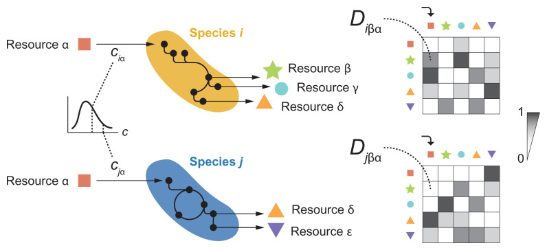
The MicroCRM (27, 29, 30) is a modeling framework based on the classic MacArthur’s consumer resource model (47). It encodes the dynamics of a system with S species and M resources in terms of a consumer preference matrix c and a metabolic matrix D, with an additional set of parameters controlling the species maintenance costs (mi for species i), the resource energy densities ( for resource α), the energy to growth rate conversion factor (gi for species i), and the leakage fraction, i.e., the amount of energy lost as byproducts when a resource is consumed ( for resource α). The element of the consumer preference matrix represents the uptake rate of resource α by species i (although the relationship between and the uptake rate can be more complex in modeling scenarios that are not considered here) (27, 29, 30). In our simulations, the elements of c are sampled from a gamma distribution and weighed so that consumers are specialized (i.e., have higher uptake rates) in a particular resource type (details in Simulations; SI Appendix; and refs. 29 and 30). Experimental evidence suggests that individual species can secrete different sets of metabolites to the environment when growing on the same primary resource (28, 37, 38). Thus, we define D as a three-dimensional matrix where the element represents the energy flux in the form of resource β that is secreted by species i when it metabolizes resource α. Note that need not be equal to if (illustration below). In the simulations, the elements of D are sampled from a Dirichlet distribution to ensure normalization, (29, 30). Other parameter values are set to the defaults of the Community Simulator (30), provided in SI Appendix.
The following equations describe the kinetics of the abundances of the ith species (denoted as Ni) and the αth resource (denoted as ):
| [1] |
| [2] |
These equations can take slightly different forms in certain cases, e.g., if the primary resource is supplied continuously instead of at the beginning of each growth cycle (29, 30). They represent a good approximation for the community dynamics between consecutive serial dilutions in our setup. Here, we assembled in silico communities by randomly sampling a set of species from a pool, then integrating Eqs. 1 and 2, diluting the final abundances, replenishing the primary resource, and repeating the process until generational equilibrium was achieved (Simulations). Coalescence simulations were carried out by mixing pairs of communities as described in the main text.
Next, to investigate the determinants of top-down coselection and the factors modulating its strength, we ran a set of simulations of community coalescence. We used a MicroCRM (27, 29) as implemented in the Community Simulator package for Python (30) (Box 1). We chose this modeling framework because communities assembled under our experimental conditions have been shown to be sustained by dense metabolic cross-feeding networks (27, 28) for which the MicroCRM provides a good description. We and others have previously found a strong concordance between the behavior of laboratory and natural microbial communities and the behavior of the MicroCRM (27, 29, 30, 35, 36). To reproduce our experimental protocol in silico, we first generated a library of resources and two nonoverlapping pools of species. A collection of 100 communities was generated from each pool (200 total) by randomly choosing 50 species and allowing them to stabilize through 20 growth–dilution cycles. We then mixed these stable communities in pairs to simulate our coalescence and dominant–dominant competition experiments (Simulations and SI Appendix). We found that the MicroCRM simulations naturally exhibit the observed correlation between the head-to-head pairwise competition of dominants and the outcome of community coalescence (Fig. 2D), further supporting the idea that top-down ecological coselection consistently emerges from metabolic interactions across species. Moreover, we found that top-down coselection is observed under a wide range of different simulation conditions and cross-feeding networks (SI Appendix, Fig. S5), indicating that it is a robust phenomenon.
Bottom-Up Coselection during Community Coalescence.
Our data indicate that the primary resource supplied to the communities can modulate the effect that the subdominants have in the dominants pairwise competition (Fig. 2C) and the strength of top-down coselection (Fig. 2B). The fact that our model captures these trends suggests that this might be a result of the metabolic interactions between community members, including the less abundant species. To investigate the potential role of the subdominant taxa in coalescence, i.e., whether the dominants may be coselected for or against by them (Fig. 1 E, Right), we ran a new set of simulations this time invading one of the communities (henceforth the nonfocal) with the dominant of the other community (henceforth the focal) alone (Simulations). We compared the invasion success of the focal dominants in isolation with respect to our previous simulations where they invaded accompanied by their ecological partners. The invasion success of the dominants was quantified as their relative abundance in the final stabilized communities (Fig. 3A). Whenever positive bottom-up ecological coselection is strong, we expect to see dominants reaching higher invasion success with their subdominant partners than by themselves, with the strongest instances occurring when dominants are unable to invade on their own but reach high densities when invading together with the other members of their communities (Fig. 3A, green shaded region). Alternatively, a high degree of bottom-up antagonism would result in dominants invading more effectively alone than in the presence of their ecological partners (Fig. 3A, red shaded region). Finally, if bottom-up coselection is weak, we would see a similar invasion success regardless of the presence or absence of the subdominant species (Fig. 3A, gray shaded region).
Fig. 3.

Trade-offs between bottom-up and top-down ecological coselections. (A) Experimental setup and hypothesis. We hypothesize that three scenarios are possible regarding bottom-up coselection: Subdominant species could coselect for (green) or against (red) their dominant in coalescence, which would result in the focal dominant reaching higher (positive bottom-up coselection) or lower (negative bottom-up coselection) abundances when accompanied by its ecological partners with respect to when invading alone. Alternatively, the subdominants could have no effect in the invasion success of the dominant taxa (no bottom-up coselection, gray). (B) Simulations with a microbial consumer-resource model: We plot the frequency reached by the focal dominants when invading the nonfocal communities in isolation versus the same frequency when invading together with their ecological partners, i.e., in community coalescence. Simulations show either weak (gray area) or strong positive (green area) bottom-up coselection, but negative bottom-up coselection is rare. (C) We divided the data from our simulations into two sets according to whether positive or no bottom-up coselection was observed (that is, whether points fell into the green or gray areas of B). Here we reproduce the plots in Fig. 2B for each set, representing the result of the dominant head-to-head pairwise competition versus the outcome of community coalescence. (Left) Strong positive bottom-up coselection (, P > 0.05). (Right) No bottom-up coselection (). (D) Experiments show that in our conditions, positive bottom-up coselection is indeed more frequent and strong than negative bottom-up coselection (red and blue dots for glutamine and citrate, respectively). (E) We reproduce the plots in C for our experimental data; i.e., we recreate Fig. 2B but this time splitting our data by the strength of bottom-up coselection instead of by the carbon source supplied to the communities. (Left) Strong positive bottom-up coselection (, P > 0.05). (Right) No bottom-up coselection ().
In our simulations of the MicroCRM, we found no instances of bottom-up antagonism but multiple such instances of positive bottom-up coselection as well as no (or weak) bottom-up coselection (Fig. 3B). Many dominant members of our in silico communities could not invade another community on their own (or could do so only at very low final relative abundances, below 0.1) but were able to reach high frequencies when they were accompanied by their subdominant partners in community coalescence. Notably, this behavior was contingent on the metabolic matrix being sparse and different for different families (i.e., need not be equal to for any two species i and j and resources α and β; Box 1), as experiments suggest is the case in natural settings (28, 37, 38) (SI Appendix, Fig. S6). Thus, theory indicates that positive bottom-up coselection is frequent and potentially very strong, while negative bottom-up coselection is far more uncommon. Interestingly, our simulations suggest that strong bottom-up coselection should be observed only in communities where top-down coselection is weak, while top-down coselection is seen only when bottom-up coselection is weak. To better illustrate this prediction, we divided our simulations into two subsets: The first one was composed of the instances where positive bottom-up coselection was strong (i.e., dots in the green shaded region in Fig. 3B), and the second set included all other cases (dots near the diagonal in Fig. 3B). We reexamined our original simulations and found that when bottom-up positive coselection is strong, the pairwise competition of dominants is not predictive of coalescence outcomes (Fig. 3 C, Left; , P > 0.05, N = 21), indicating that top-down coselection is weak. At the same time, when considering only those coalesced communities in the diagonal in Fig. 3B (where bottom-up coselection is weak), our model predicts that the fates of the subdominant community members after coalescence are more strongly determined by the head-to-head competition between dominants in isolation (, N = 79 for instances where bottom-up coselection is weak [Fig. 3 C, Right]; , , N = 100 when all instances are considered [Fig. 2D]).
We then asked whether this behavior predicted by the model was also observed in our experimental communities. To address this question, we carried out a new round of experiments where we invaded the nonfocal communities with the dominants of the focal communities alone (Coalescence, Competition, and Invasion Experiments). After stabilization (Stabilization of Environmental Communities in Simple Synthetic Environments), we quantified species abundance through 16S Illumina sequencing (Determination of Community Composition by 16S Sequencing). Consistent with the behavior of our model, we observed that whenever bottom-up coselection is seen, it is always positive and we do not see any instances of antagonistic coselection (Fig. 3D). Interestingly, bottom-up recruitment appears to be more frequent in the glutamine environments, where top-down coselection was weak, than in the citrate ones, where top-down coselection was strong (Fig. 2). We then repeated our analysis in Fig. 3C, this time splitting our data according to the observed strength of bottom-up coselection instead of the primary carbon source as we had done in Fig. 2B. Our findings were in line with the model prediction: Pairwise competition between dominants is predictive of coalescence outcomes only if bottom-up coselection is weak (Fig. 3E; , P > 0.05, N = 14 when bottom-up coselection is strong; , N = 42 when bottom-up coselection is weak). Once the bottom-up communities are removed, both the glutamine and citrate communities display similar degrees of top-down cohesiveness (Fig. 3 E, Right). This suggests that the main difference between citrate and glutamine habitats from the standpoint of community coalescence is that the latter is richer in communities exhibiting bottom-up cohesiveness than the former. When this difference is factored out, both behave similarly.
Understanding the Mechanisms of Ecological Coselection: A Minimal Model of Community Coalescence.
In view of the success of our model in reproducing the experimentally observed trends in ecological coselection, we set out to better understand the mechanisms for its emergence. In our experimental conditions and in the MicroCRM simulations, communities are sustained by dense cross-feeding facilitation networks. These networks can have a very vertical, top-down structure if a single species (the dominant) cross-feeds the less abundant members of the community but these do not cross-feed the dominant in return. Alternatively, if the dominant is strongly cross-fed by the less abundant species in the community, the network structure would be more horizontal. In the latter scenario, positive bottom-up coselection of a dominant can take place if cross-feeding from its ecological partners allows it to persist in the final community after coalescence—even if it cannot invade successfully in isolation.
We found it useful to study a minimal model of community coalescence to test these ideas (MinimalModel). This model is composed of two communities (focal and nonfocal) with only two species each as illustrated in Fig. 4A. Within each community, the dominant species ( and , respectively) are able to utilize the single externally supplied resource (). They secrete a single byproduct ( and , respectively) off which the subdominants ( and , respectively) can feed. Finally, these subdominants secrete an additional resource ( and , respectively). The dominants’ ability to utilize their subdominants’ metabolic byproducts determines whether the structure of the cross-feeding networks of these minimal communities is vertical (if the dominants cannot utilize the subdominants’ secretions and thus are not cross-fed by them) or horizontal (in the opposite scenario). The rates controlling how effectively the dominants can metabolize said byproducts modulate the direction of the cross-feeding networks (Fig. 4A). The model is thus specified by four parameters: the uptake rate of the primary resource by the focal dominant, c11; the uptake rate of the primary resource by the nonfocal dominant, ; the uptake rate of the byproduct by the focal dominant, c13; and the uptake rate of the byproduct by the nonfocal dominant, .
Fig. 4.

A minimal model of community coalescence. (A) Illustration of the model structure and parameters. The primary resource () is replenished after each growth–dilution cycle (red arrows). Solid arrows indicate resource consumption, and dashed arrows represent resource secretion. (B–E) Coalescence outcomes in the minimal model under different relations of cohesiveness between the focal and nonfocal communities. We represent the relative Bray–Curtis similarity between the focal and the coalesced communities (Q) as a function of the relevant model parameters. For the specific representative cases indicated by the open circles, we also show Q as a function of the frequency of the focal dominant in pairwise competition with the nonfocal dominant, as well as the frequency of the focal dominant invading alone versus invading accompanied by its subdominant partner.
In the limit case when the cross-feeding networks of both communities are strictly vertical (that is, the subdominants are passively sustained by the dominants but do not cross-feed them), but also different in the resources each secretes, it is straightforward that the outcome of community coalescence will depend on the competitive ability of the dominants to grow on the single externally supplied resource. The most competitive dominant will coselect its subdominant (i.e., top-down coselection) through the secretion of specific metabolic byproducts that it can consume (but that the subdominant of the other community cannot) as shown in Fig. 4B. If the nonfocal community is maintained by a more horizontal cross-feeding network, it can display further resistance to invasion by the vertical focal community. In this case, even if the focal dominant is more competitive for the externally supplied resource than the nonfocal dominant, the nonfocal community could still dominate in coalescence due to cross-feeding from the subdominant favoring the dominant. The stronger the bottom-up metabolic flux from the nonfocal subdominant toward its dominant, the more prominent this effect can be (Fig. 4C). The situation could become more interesting when the focal (Fig. 4D) or both the focal and the nonfocal communities (Fig. 4E) exhibit a horizontal cross-feeding network. In both of these scenarios, cross-feeding from the focal subdominant could favor the persistence of the focal community in coalescence even when the focal dominant is less competitive for the primary resource in head-to-head pairwise competition (and therefore cannot invade in isolation).
In summary, thinking through our minimal model tells us that coalescence outcomes should be contingent on the direction of the cross-feeding networks sustaining the communities in this simple setting. To verify our intuitive reasoning, we ran simulations of all scenarios described above with our minimal model of community coalescence implemented in the MicroCRM framework (Minimal Model and SI Appendix). In line with our initial proposition, simulations indicate that bottom-up coselection of a dominant that is unable to invade by itself is possible if said dominant is strongly cross-fed by its ecological partner (Fig. 4).
Community Hierarchy Regulates the Strength of Bottom-Up Coselection.
How do the ideas above scale to more complex and diverse communities? In natural microbiomes and in our laboratory cultures, a large number of species can coexist and cross-feed each other, giving rise to facilitation networks that are far denser than the ones in our minimal model. To generalize the intuition gained in Fig. 4 to communities with more than two species, we introduce a hierarchy index h that quantifies how vertical a cross-feeding network is:
| [3] |
where represents the overall increase in dominant biomass within a single batch incubation for a generationally stable community, and represents the increase in said biomass resulting from the metabolism of the primary resource () only. If the dominant was utilizing just the primary resource, the cross-feeding network would be very vertical (), whereas if it was growing mostly on the secretions of other taxa, it would be more horizontal (). We quantified the hierarchies of the communities in our MicroCRM simulations, finding that h follows a bimodal distribution (Fig. 5A). We therefore divided our simulations into four groups according to whether the cross-feeding networks of both focal and nonfocal communities were vertical (“high h” when h > 0.25) or horizontal (“low h” when h < 0.25) as shown in Fig. 5B. For each group, we evaluated the frequency of instances of bottom-up coselection, i.e., the fraction of cases where a dominant that could not invade in isolation was successful when accompanied by its ecological partners (green area in Fig. 3B). We found that bottom-up ecological coselection is significantly more frequent when the focal community is nonhierarchical (Fig. 5C), in line with what the minimal model anticipated (Fig. 4).
Fig. 5.

Community hierarchy modulates the recurrence of bottom-up coselection. (A) Distribution of community hierarchies for our in silico communities. (B) We divided our coalescence simulations into four groups according to the hierarchies of the focal () and nonfocal () communities as indicated by the dashed boxes. For every group, we calculated the fraction of cases where bottom-up coselection was observed; i.e., the focal dominant was unsuccessful when invading in isolation but successful when invading with its ecological partners. (C) Bottom-up coselection of the focal dominant during coalescence is significantly more frequent when the focal community is nonhierarchical. Error bars representing 95% confidence intervals and P values were computed by bootstrapping (**** where indicated).
Conclusions
Understanding the mechanisms underlying the responses of microbial communities to invasions is an essential but poorly understood question in microbial ecology (10). Theory has suggested that communities may exhibit an emergent cohesiveness (11, 12, 18, 19), leading to members of the same community recruiting one another during community–community invasions. Our results provide direct experimental evidence of ecological coselection in a large number of community coalescence experiments and highlight the critical role that may be played by the rarer, subdominant species in the generation of community cohesiveness.
Our simulations suggest that the strength and direction of ecological coselection may be modulated by the underlying cross-feeding networks that shape the structure of communities in synthetic minimal environments (27, 28). This idea is supported by the observation that our microbial consumer-resource model captures the trends observed experimentally when we enable a large variation in the metabolic fluxes across species. The model predicts a trade-off between the strength of bottom-up coselection and the ability of dominant–dominant pairwise competition to dictate coalescence outcomes, which we have confirmed experimentally. It also suggests that rarer taxa may play a more prominent role in coselecting dominant species when the cross-feeding interactions across community members are horizontal rather than hierarchical. Testing this theoretical prediction would require one to map the cross-feeding networks of all of our communities. Keeping track of every nutrient secreted by every species in coculture and by which species they are uptaken is still a low-throughput process that is both labor intensive and expensive, but recent progress in metabolomic tools promise to help us test this hypothesis in future work. Our findings, together with previous results in different systems (22) as well as theoretical predictions (11, 18–21), suggest that collective interactions of microbes with one another and with the environment should be generically expected to produce ecological coselection during community coalescence.
Materials and Methods
Stabilization of Environmental Communities in Simple Synthetic Environments.
Communities were stabilized ex situ as described in ref. 27. In short, environmental samples (soil, leaves, …) within 1 m radius in eight different geographical locations were collected with sterile tweezers or spatulas into 50-mL sterile tubes (Fig. 1A). One gram of each sample was allowed to sit at room temperature in 10 mL of phosphate-buffered saline (1× PBS) containing 200 µg/mL cycloheximide to suppress eukaryotic growth. After 48 h, samples were mixed 1:1 with 80% glycerol and kept frozen at C. Starting microbial communities were prepared by scraping the frozen stocks into 200 µL of 1× PBS and adding a volume of 4 µL to 500 µL of synthetic minimal media (1× M9) supplemented with 200 µg/mL cycloheximide and 0.07 C-mol/L glutamine or sodium citrate as the carbon source in 96 deep-well plates (1.2 mL; VWR). Cultures were then incubated still at C to allow for regrowth. After 48 h, samples were fully homogenized and biomass increase was followed by measuring the optical density (620 nm) of 100 µL of the cultures in a Multiskan FC plate reader (Thermo Scientific). Communities were stabilized (27) by passaging 4 µL of the cultures into 500 µL of fresh media (1× M9 with the carbon source) every 48 h for a total of 12 transfers at a dilution factor of 1:100, roughly equivalent to 80 generations per culture (Fig. 1B). Cycloheximide was not added to the media after the first two transfers.
Isolation of Dominant Species.
For each community, the most abundant colony morphotype at the end of the ninth transfer was selected (Fig. 1C), resuspended in 100 µL 1× PBS, and serially diluted (1:10). Next, 20 µL of the cells diluted to were plated in the corresponding synthetic minimal media and allowed to regrow at C for 48 h. Dominants were then identified, inoculated into 500 µL of fresh media, and incubated still at C for 48 h. After this period, the communities stabilized for 11 transfers and the isolated dominants were ready for the competition experiments at the onset of the 12th transfer.
Isolation of Subdominant Species and Fitness Estimation.
Citrate communities were diluted to and plated in chromogenic agar plates (CHROMagar Mastitis GN). All visible colony morphotypes (including the less abundant, subdominant ones) were selected. For each morphotype, a single colony was resuspended in 100 µL of 1× PBS and 5 µL of the suspension was transferred to 500 µL of synthetic minimal media (1× M9) containing 0.07 C-mol/L sodium citrate in 96-well deep-well plates. A total of 100 µL of the cultures was transferred to a 96-well flat-bottom plate and placed in a Multiskan FC plate reader. Growth was tracked by measuring the optical density (OD) at 620 nm every 10 min for 24 h. In addition, species were grown in the spent media of their respective dominants following the same protocol. Spent media were obtained by resuspending a single colony of the dominant species in 20 mL of synthetic citrate media in 50 mL Falcon tubes, allowing it to grow for 24 h, and then centrifuging the tubes at 3,500 rpm for 25 min to pellet the cells. Supernatants were collected and filtered using a 0.2-µm filter (Thermo Scientific Nalgene Rapid-Flow). Filtered supernatants of each dominant were used to grow the corresponding subdominants as described above. Fitness in both the primary citrate environment and the dominants’ spent media was estimated as the average growth rate over the first 15 h.
Coalescence, Competition, and Invasion Experiments.
All possible pairwise dominant–dominant and community–community competition experiments were performed by mixing equal volumes (4 µL) of each of the eight communities or eight dominants at the onset of the 12th transfer. Competitions were set up in their native media, i.e., in 500 µL of 1× M9 supplemented with 0.07 C-mol/L of either glutamine or citrate in 96-well deep-well plates. Plates were incubated at C for 48 h. Pairwise competitions were further propagated for seven serial transfers (roughly 42 generations, Fig. 1F) by transferring 8 µL of each culture to fresh media (500 µL).
Determination of Community Composition by 16S Sequencing.
The sequencing protocol was identical to that described in ref. 27. Community samples were collected by spinning down at 3,500 rpm for 25 min in a bench-top centrifuge at room temperature; cell pellets were stored at C before processing. To maximize Gram-positive bacteria cell wall lysis, the cell pellets were resuspended and incubated at C for 30 min in enzymatic lysis buffer (20 mM Tris HCl, 2 mM sodium ethylenediamine tetraacetic acid (EDTA), 1.2% Triton X-100) and 20 mg/mL of lysozyme from chicken egg white (Sigma-Aldrich). After cell lysis, the DNA extraction and purification were performed using the DNeasy 96 protocol for animal tissues (Qiagen). The clean DNA in 100 µL elution buffer of 10 mM TrisHCl, 0.5 mM EDTA at pH 9.0 was quantified using a Quan-iT PicoGreen dsDNA Assay Kit (Molecular Probes, Inc.) and normalized to 5 ng/µL in nuclease-free water (Qiagen) for subsequent 16S rRNA Illumina sequencing. The 16S rRNA amplicon library preparation was performed following a dual-index paired-end approach (39). Briefly, PCR amplicon libraries of V4 regions of the 16S rRNA were prepared using dual-index primers (F515/R805) and then pooled and sequenced using the Illumina MiSeq chemistry and platform. Each sample went through a 30-cycle PCR in duplicate of 20 µL reaction volumes using 5 ng of DNA each, dual index primers, and AccuPrime Pfx SuperMix (Invitrogen). The thermocycling procedure includes a 2-min initial denaturation step at C and 30 cycles of the following PCR scheme: 1) a 20-s denaturation at C, 2) 15-s annealing at C, and 3) 5-min extension at C. The duplicate PCR products of each sample were pooled, purified, and normalized using a SequalPrep PCR cleanup and normalization kit (Invitrogen). Barcoded amplicon libraries were then pooled and sequenced using the Illumina Miseq v2 reagent kit, which generated 2 × 250-bp paired-end reads at the Yale Center for Genome Analysis (YCGA). The sequencing reads were demultiplexed on QIIME 1.9.0 (40). The barcodes, indexes, and primers were removed from raw reads, producing FASTQ files with both the forward and reverse reads for each sample, ready for DADA2 analysis (34). DADA2 version 1.1.6 was used to infer unique biological exact sequence variants (ESVs) for each sample and naive Bayes was used to assign taxonomy using the SILVA version 123 database (41, 42).
Metrics of Community Distance.
Beta-diversity indexes between communities were computed using various similarity metrics. For two arbitrary communities with ESV abundances represented by the vectors and (where xi and yi are the relative abundances of the ith ESV in each community, respectively, and S is the total number of ESVs), the Bray–Curtis similarity (BC) index is calculated as (43)
| [4] |
The Jensen–Shannon similarity (JS) is defined as one minus the Jensen–Shannon distance (which is, in turn, the square root of the Jensen–Shannon divergence) (44)
| [5] |
where and KL denotes the Kullback–Leibler divergence (45)
| [6] |
Using base-2 logarithms ensures that JS is bounded between 0 and 1. The Jaccard similarity (J) is given by (46):
| [7] |
Additionally, we quantified coalescence outcomes by examining the fraction of the endemic taxa of the original communities that persisted in the coalesced one. We call the fraction of endemic species of x that are also found in y.
For all the metrics above, we quantified the relative similarity between one of the primary communities (community A) and the coalesced community using relative metrics (denoted as Q):
| [8] |
where the subscripts A and B correspond to the primary communities, the subscript C corresponds to the final community after coalescence, and F represents one of BC, JS, J, or E (endemic survival) defined above.
Simulations.
We used the Community Simulator package (30) and included additional features for our simulations. In the package, species are characterized by their resource uptake rates ( for species i and resource α), and they all share a common metabolic matrix D. The element Dαβ of this matrix represents the fraction of energy in the form of resource α secreted when resource β is consumed. Here we implemented a regime in which species can secrete different metabolites (and/or in different abundances) when consuming a same resource. We call the fraction of energy in the form of resource α secreted by species i when consuming resource β. Details on parameter sampling are provided in SI Appendix. For our simulations, we first generated a library of 2,640 species divided into three specialist families of 800 members each and a generalist family of 240 members, as well as a library of 30 resources divided into three classes of 10 each. Species differ from one another in their resource uptake rates and in the type and abundance of byproducts they secrete (details in SI Appendix). We split the library of consumers into two nonoverlapping pools of 1,320 species each. We randomly sampled 50 species from each pool in equal ratios to seed 200 communities (100 from each pool). We then let grow and diluted the communities serially, replenishing the primary resource after each dilution. We repeated the process 20 times to ensure generational equilibrium was achieved (27). We then performed the in silico experiments by using the generationally stable communities to seed 100 coalesced communities that were again stabilized as described previously. Similarly, we identified the dominant (most abundant) species of every community to carry out pairwise competition and single invasion simulations.
Minimal Model.
Our minimal model is set within the same MicroCRM framework that we used for the previous simulations. As described in the main text, the model contains two communities of two species each ( and in the focal community, and in the nonfocal community), with five resources in total, of which the first one () is replenished externally at the beginning of each growth cycle and the rest correspond to the species’ metabolic byproducts (Fig. 4A). Each species secretes a unique byproduct, meaning that the metabolic matrix D is binary in this case. The specific form of the matrices c and D is provided in SI Appendix. We ran simulations of this model for each one of the scenarios considered in Fig. 4, varying the corresponding rates within the specified limits. Whenever we were interested in the ratio between two rates (e.g., in Fig. 4E) we gave the one in the denominator a fixed value of 1 and shifted the one in the numerator to cover the range of interest.
Supplementary Material
Acknowledgments
Work in A.S.’s laboratory is supported by NIH Grant 1R35 GM133467-01 and by a Packard Fellowship from the David and Lucille Packard Foundation. The funding for this work partly results from a Scialog Program sponsored jointly by the Research Corporation for Science Advancement and the Gordon and Betty Moore Foundation through grants to Yale University by the Research Corporation and the Simons Foundation. We thank Pankaj Mehta, Wenping Cui, Robert Marsland, and all members of A.S.’s laboratory for many helpful discussions. We also express our gratitude to the Goodman laboratory at Yale University for technical help during the early stages of this project.
Footnotes
The authors declare no competing interest.
This article is a PNAS Direct Submission. S.L. is a guest editor invited by the Editorial Board.
This article contains supporting information online at https://www.pnas.org/lookup/suppl/doi:10.1073/pnas.2111261119/-/DCSupplemental.
Data Availability
Experimental data and code for the analysis, as well as code for the simulations and the updated Community Simulator package with instructions for enabling the additional features, can be found in GitHub at http://github.com/jdiazc9/coalescence. All data and code has been deposited in Zenodo at https://doi.org/10.5281/zenodo.5879150 (48).
References
- 1.Mansour I., Heppell C. M., Ryo M., Rillig M. C., Application of the microbial community coalescence concept to riverine networks. Biol. Rev. Camb. Philos. Soc. 93, 1832–1845 (2018). [DOI] [PubMed] [Google Scholar]
- 2.Luo X, et al., Seasonal effects of river flow on microbial community coalescence and diversity in a riverine network. FEMS Microbiol. Ecol. 96, fiaa132 (2020). [DOI] [PubMed] [Google Scholar]
- 3.Vass M., Székely A. J., Lindström E. S., Osman O. A., Langenheder S., Warming mediates the resistance of aquatic bacteria to invasion during community coalescence. Mol. Ecol. 30, 1345–1356 (2021). [DOI] [PubMed] [Google Scholar]
- 4.Rillig M. C., et al., Soil microbes and community coalescence. Pedobiologia (Jena) 59, 37–40 (2016). [Google Scholar]
- 5.Ramoneda J., et al., Soil microbial community coalescence and fertilization interact to drive the functioning of the legume–rhizobium symbiosis. J. Appl. Ecol. 00, 1–13 (2021). [Google Scholar]
- 6.Rochefort A., et al., Transmission of seed and soil microbiota to seedling. mSystems 6, e00446–21 (2021). [DOI] [PMC free article] [PubMed] [Google Scholar]
- 7.Evans S. E., Bell-Dereske L. P., Dougherty K. M., Kittredge H. A., Dispersal alters soil microbial community response to drought. Environ. Microbiol. 22, 905–916 (2020). [DOI] [PubMed] [Google Scholar]
- 8.C. L. Dutton, et al., The meta-gut: Hippo inputs lead to community coalescence of animal and environmental microbiomes. bioRxiv [Preprint] (2021). https://www.biorxiv.org/content/10.1101/2021.04.06.438626v1 (Accessed 15 May 2021).
- 9.Vandegrift R., et al., Moving microbes: The dynamics of transient microbial residence on human skin. bioRxiv [Preprint] (2019). https://www.biorxiv.org/content/10.1101/586008v1 (Accessed 15 May 2021).
- 10.Rillig M. C., et al., Interchange of entire communities: Microbial community coalescence. Trends Ecol. Evol. 30, 470–476 (2015). [DOI] [PubMed] [Google Scholar]
- 11.Gilpin M., Community-level competition: Asymmetrical dominance. Proc. Natl. Acad. Sci. U.S.A. 91, 3252–3254 (1994). [DOI] [PMC free article] [PubMed] [Google Scholar]
- 12.Livingston G., Jiang Y., Fox J. W., Leibold M. A., The dynamics of community assembly under sudden mixing in experimental microcosms. Ecology 94, 2898–2906 (2013). [DOI] [PubMed] [Google Scholar]
- 13.Prior K. M., Robinson J. M., Meadley Dunphy S. A., Frederickson M. E., Mutualism between co-introduced species facilitates invasion and alters plant community structure. Proc. Biol. Sci. 282, 20142846 (2015). [DOI] [PMC free article] [PubMed] [Google Scholar]
- 14.Castledine M., Sierocinski P., Padfield D., Buckling A., Community coalescence: An eco-evolutionary perspective. Philos. Trans. R. Soc. Lond. B Biol. Sci. 375, 20190252 (2020). [DOI] [PMC free article] [PubMed] [Google Scholar]
- 15.Rillig M. C., Tsang A., Roy J., Microbial community coalescence for microbiome engineering. Front. Microbiol. 7, 1967 (2016). [DOI] [PMC free article] [PubMed] [Google Scholar]
- 16.Rocca J. D., Muscarella M. E., Peralta A. L., Izabel-Shen D., Simonin M., Guided by microbes: Applying community coalescence principles for predictive microbiome engineering. mSystems 6, e00538–21 (2021). [DOI] [PMC free article] [PubMed] [Google Scholar]
- 17.Chang C. Y., et al., Engineering complex communities by directed evolution. Nat. Ecol. Evol. 5, 1011–1023 (2021). [DOI] [PMC free article] [PubMed] [Google Scholar]
- 18.Tikhonov M., Community-level cohesion without cooperation. eLife 5, e15747 (2016). [DOI] [PMC free article] [PubMed] [Google Scholar]
- 19.Tikhonov M., Monasson R., Collective phase in resource competition in a highly diverse ecosystem. Phys. Rev. Lett. 118, 048103 (2017). [DOI] [PubMed] [Google Scholar]
- 20.Vila J. C. C., Jones M. L., Patel M., Bell T., Rosindell J., Uncovering the rules of microbial community invasions. Nat. Ecol. Evol. 3, 1162–1171 (2019). [DOI] [PubMed] [Google Scholar]
- 21.Lechón-Alonso P., Clegg T., Cook J., Smith T. P., Pawar S., The role of competition versus cooperation in microbial community coalescence. PLoS Comput. Biol. 17, e1009584 (2021). [DOI] [PMC free article] [PubMed] [Google Scholar]
- 22.Sierocinski P., et al., A single community dominates structure and function of a mixture of multiple methanogenic communities. Curr. Biol. 27, 3390–3395.e4 (2017). [DOI] [PubMed] [Google Scholar]
- 23.Rillig M. C., Mansour I., Microbial ecology: Community coalescence stirs things up. Curr. Biol. 27, R1280–R1282 (2017). [DOI] [PubMed] [Google Scholar]
- 24.Louca S., et al., High taxonomic variability despite stable functional structure across microbial communities. Nat. Ecol. Evol. 1, 0015 (2016). [DOI] [PubMed] [Google Scholar]
- 25.Winfree R., . Fox J. W, Williams N. M., Reilly J. R., Cariveau D. P., Abundance of common species, not species richness, drives delivery of a real-world ecosystem service. Ecol. Lett. 18, 626–635 (2015). [DOI] [PubMed] [Google Scholar]
- 26.Rosenzweig R. F., Sharp R. R., Treves D. S., Adams J., Microbial evolution in a simple unstructured environment: Genetic differentiation in Escherichia coli. Genetics 137, 903–917 (1994). [DOI] [PMC free article] [PubMed] [Google Scholar]
- 27.Goldford J. E., et al., Emergent simplicity in microbial community assembly. Science 361, 469–474 (2018). [DOI] [PMC free article] [PubMed] [Google Scholar]
- 28.Estrela S., et al., Functional attractors in microbial community assembly. Cell Syst.S2405-4712(21)00379-3 10.1016/j.cels.2021.09.011. (2021). [DOI] [PMC free article] [PubMed] [Google Scholar]
- 29.Marsland 3rd R., et al., Available energy fluxes drive a transition in the diversity, stability, and functional structure of microbial communities. PLOS Comput. Biol. 15, e1006793 (2019). [DOI] [PMC free article] [PubMed] [Google Scholar]
- 30.Marsland R., Cui W., Goldford J., Mehta P., The Community Simulator: A Python package for microbial ecology. PLoS One 15, e0230430 (2020). [DOI] [PMC free article] [PubMed] [Google Scholar]
- 31.Dimroth P., Molecular basis for bacterial growth on citrate or malonate. Ecosal Plus, 10.1128/ecosalplus.3.4.6 (2004). [DOI] [PubMed] [Google Scholar]
- 32.Forchhammer K., Glutamine signalling in bacteria. Front. Biosci. 12, 358–370 (2007). [DOI] [PubMed] [Google Scholar]
- 33.Callahan B. J., et al., DADA2: High-resolution sample inference from Illumina amplicon data. Nat. Methods 13, 581–583 (2016). [DOI] [PMC free article] [PubMed] [Google Scholar]
- 34.Callahan B. J., McMurdie P. J., Holmes S. P., Exact sequence variants should replace operational taxonomic units in marker-gene data analysis. ISME J. 11, 2639–2643 (2017). [DOI] [PMC free article] [PubMed] [Google Scholar]
- 35.Marsland 3rd R., Cui W., Mehta P., A minimal model for microbial biodiversity can reproduce experimentally observed ecological patterns. Sci. Rep. 10, 3308 (2020). [DOI] [PMC free article] [PubMed] [Google Scholar]
- 36.Estrela S., Sanchez-Gorostiaga A., Vila J. C., Sanchez A., Nutrient dominance governs the assembly of microbial communities in mixed nutrient environments. eLife 10, e65948 (2021). [DOI] [PMC free article] [PubMed] [Google Scholar]
- 37.Harcombe W. R., et al., Metabolic resource allocation in individual microbes determines ecosystem interactions and spatial dynamics. Cell Rep. 7, 1104–1115 (2014). [DOI] [PMC free article] [PubMed] [Google Scholar]
- 38.Pinu F. R., et al., Metabolite secretion in microorganisms: The theory of metabolic overflow put to the test. Metabolomics 14, 43 (2018). [DOI] [PubMed] [Google Scholar]
- 39.Kozich J. J., Westcott S. L., Baxter N. T., Highlander S. K., Schloss P. D., Development of a dual-index sequencing strategy and curation pipeline for analyzing amplicon sequence data on the MiSeq Illumina sequencing platform. Appl. Environ. Microbiol. 79, 5112–5120 (2013). [DOI] [PMC free article] [PubMed] [Google Scholar]
- 40.Caporaso J. G., et al., QIIME allows analysis of high-throughput community sequencing data. Nat. Methods 7, 335–336 (2010). [DOI] [PMC free article] [PubMed] [Google Scholar]
- 41.Wang Q., Garrity G. M., Tiedje J. M., Cole J. R., Naive Bayesian classifier for rapid assignment of rRNA sequences into the new bacterial taxonomy. Appl. Environ. Microbiol. 73, 5261–5267 (2007). [DOI] [PMC free article] [PubMed] [Google Scholar]
- 42.Quast C., et al., The SILVA ribosomal RNA gene database project: Improved data processing and web-based tools. Nucleic Acids Res. 41, D590–D596 (2013). [DOI] [PMC free article] [PubMed] [Google Scholar]
- 43.Curtis J. T., Bray J. R., An ordination of the upland forest communities of Southern Wisconsin. Ecol. Monogr. 27, 325–349 (1957). [Google Scholar]
- 44.Lin J., Divergence measures based on the Shannon entropy. IEEE Trans. Inf. Theory 37, 145–151 (1991). [Google Scholar]
- 45.Kullback S., Leibler R. A., On information and sufficiency. Ann. Math. Stat. 22, 79–86 (1951). [Google Scholar]
- 46.Jaccard P., The distribution of the flora in the Alpine zone. New Phytol. 11, 37–50 (1912). [Google Scholar]
- 47.MacArthur R., Species packing and competitive equilibrium for many species. Theor. Popul. Biol. 1, 1–11 (1970). [DOI] [PubMed] [Google Scholar]
- 48.Diaz-Colunga J., coalescence-20210617. Zenodo. 10.5281/zenodo.5879150. Deposited 17 June 2021. [DOI]
Associated Data
This section collects any data citations, data availability statements, or supplementary materials included in this article.
Supplementary Materials
Data Availability Statement
Experimental data and code for the analysis, as well as code for the simulations and the updated Community Simulator package with instructions for enabling the additional features, can be found in GitHub at http://github.com/jdiazc9/coalescence. All data and code has been deposited in Zenodo at https://doi.org/10.5281/zenodo.5879150 (48).