Time-resolved DEER EPR and solid-state NMR afford kinetic and structural elucidation of substrate binding to Ca²⁺-ligated calmodulin

Significance

Complex formation between calmodulin and target proteins underlies numerous calcium signaling processes in biology, yet structural and mechanistic details, which entail major conformational changes in both calmodulin and its substrates, have been unclear. We show that a combination of time-resolved electron paramagnetic and NMR measurements can elucidate the molecular mechanism, at the quantitative kinetic and structural levels, of the binding pathway of a peptide substrate from skeletal muscle myosin light-chain kinase to calcium-loaded calmodulin. The mechanism involves coupled folding and binding and comprises a bifurcated process, with rapid, direct complex formation when the peptide interacts first with the C-terminal domain of calmodulin or a slower, two-step complex formation when the peptide interacts initially with the N-terminal domain.

Abstract

Recent advances in rapid mixing and freeze quenching have opened the path for time-resolved electron paramagnetic resonance (EPR)-based double electron-electron resonance (DEER) and solid-state NMR of protein–substrate interactions. DEER, in conjunction with phase memory time filtering to quantitatively extract species populations, permits monitoring time-dependent probability distance distributions between pairs of spin labels, while solid-state NMR provides quantitative residue-specific information on the appearance of structural order and the development of intermolecular contacts between substrate and protein. Here, we demonstrate the power of these combined approaches to unravel the kinetic and structural pathways in the binding of the intrinsically disordered peptide substrate (M13) derived from myosin light-chain kinase to the universal eukaryotic calcium regulator, calmodulin. Global kinetic analysis of the data reveals coupled folding and binding of the peptide associated with large spatial rearrangements of the two domains of calmodulin. The initial binding events involve a bifurcating pathway in which the M13 peptide associates via either its N- or C-terminal regions with the C- or N-terminal domains, respectively, of calmodulin/4Ca²⁺ to yield two extended “encounter” complexes, states A and A*, without conformational ordering of M13. State A is immediately converted to the final compact complex, state C, on a timescale τ ≤ 600 μs. State A*, however, only reaches the final complex via a collapsed intermediate B (τ ∼ 1.5 to 2.5 ms), in which the peptide is only partially ordered and not all intermolecular contacts are formed. State B then undergoes a relatively slow (τ ∼ 7 to 18 ms) conformational rearrangement to state C.

Calmodulin (CaM) is a universal eukaryotic calcium sensor that plays a central role in calcium signaling (1). Binding of two Ca²⁺ ions per CaM domain exposes methionine-rich hydrophobic patches that prime the system for high-affinity binding to a wide range of protein partners (2). Free calcium–loaded calmodulin (CaM/4Ca²⁺) is predominantly extended (3–5), although sparsely populated, highly transient compact states are sampled (6, 7), but clamps down upon target substrates like two hands capturing a rope in the final complex (8–11) (Fig. 1). Concomitant conformational changes involve the transition of a largely helical interdomain linker to a long flexible loop and the adoption of a helical conformation by the intrinsically disordered substrate. Although CaM has been the subject of extensive biophysical studies (12–16), current structural knowledge is limited to calcium-free, calcium-loaded, and calcium-loaded/peptide-bound states as separate entities, with little experimental information about the molecular mechanisms that connect the latter two states. For example, it is not known whether substrates bind first to the N-terminal domain (NTD) or C-terminal domain (CTD) of CaM/4Ca²⁺, whether identifiable intermediate states exist, whether there is a single predominant pathway for complex formation, or at what stage in the process the CaM binding regions of target protein substrates become conformationally ordered. To address this knowledge gap, we have performed time-resolved electron paramagnetic resonance (EPR)-based double electron-electron resonance (DEER) and solid-state (ss) NMR studies that jointly elucidate the process of CaM/4Ca²⁺–peptide complex formation in quantitative kinetic and structural terms. This work relies on three technological advances: 1) rapid mixing and freeze quenching to sequentially trap the state of the reaction mixture on the millisecond timescale (17–24), thereby permitting time-resolved DEER EPR and ssNMR measurements of protein–substrate interactions; 2) the application of phase-memory time (T_m) filtering (25) to quantitatively extract species populations from DEER data (26) so that time-dependent probability distance distributions between pairs of spin labels can be monitored; and 3) quantitative analysis of ssNMR ¹³C-¹³C correlation spectra to provide residue-specific information on the appearance of structural order and the development of intermolecular contacts between substrate and protein (21, 23).

Fig. 1.

Schematic overview of the time-resolved DEER EPR and ssNMR experiments. The predominant extended conformation of free CaM/4Ca²⁺ seen in the crystal structure is shown in Upper Left (3); the locations of the R1 nitroxide spin labels (transparent red spheres) at A17C–R1 and A128C–R1 in the NTD (blue) and CTD (purple), respectively, and of the relevant methionine residues (gray balls) are indicated. The intrinsically disordered M13 peptide, comprising the CaM binding site of skMLCK, is shown in Upper Right, with ¹³C-labeled residues in the N- and C-terminal halves of the peptides shown as blue and mauve balls, respectively. The structure of the final CaM/4Ca²⁺–M13 complex (8, 9) is shown in Lower, with the helical M13 peptide in red. The reaction time is controlled by the flow rate through the mixer and the flight distance from the mixer nozzle to the spinning copper disk cooled to 77K.

Results

Experimental Design and Setup.

DEER EPR (27) provides distance distributions, P(r), for pairs of nitroxide spin labels (26) covalently attached to surface cysteine residues introduced by site-directed mutagenesis (28). Here, the R1 nitroxide spin labels (29) are located at S17C and A128C in the NTD and CTD of CaM, respectively, thereby affording global structural information related to the positioning of the two domains with respect to one another. The introduction of R1 labels at A17C–R1 and A128C–R1 entails no observable structural perturbation in CaM/4Ca²⁺ and only reduces the affinity for the M13 substrate about 2.5-fold (6). CaM and the solvent were fully deuterated to maximize the phase memory relaxation times (T_m), thereby both increasing signal to noise and the accuracy with which longer distances can be determined (30, 31). The synthetic 26-residue peptide substrate, known as M13, comprising the CaM binding site of skeletal muscle myosin light chain kinase (skMLCK), however, was fully protonated, allowing us to exploit T_m filtering (25) to extract accurate populations of components within P(r) (see below).

For ssNMR measurements, M13 was ¹³C labeled at residues K5, F8, V11, A13, F17, and I20 (Figs. 1 and 2A), thereby permitting site-specific assessments of the development of α-helical conformational order in M13 upon interaction with CaM/4Ca²⁺ from intramolecular cross-peak line shapes in two-dimensional (2D) ¹³C-¹³C correlation spectra with a spin-diffusion mixing period, τ_SD = 20 ms (23). In addition, all methionines of CaM were ¹³C_methyl labeled (Fig. 1) to monitor the appearance of intermolecular contacts between CaM and M13 using τ_SD = 1 s to generate strong intermolecular M13–CaM cross-peaks via homonuclear dipole–dipole interactions with a distance of ≤8 Å (23).

Fig. 2.

Samples and mixing setup for time-resolved DEER EPR and ssNMR experiments. (A) Sites of ¹³C labeling of the M13 peptide for ssNMR. (B) Mixing conditions for rapid freeze quenching. The reaction time (t_r) comprises the mixing time and the time to reach the copper plate, and was varied from 1.5 to 25 ms; freezing occurs within 0.5 ms. The t_r = 0 (i.e., free CaM/4Ca²⁺) and t_r = ∞ (i.e., final CaM/4Ca²⁺–M13 complex) samples were prepared using the identical mixing procedure. For the former, M13 is omitted from the second "syringe" (on the left); for the latter, M13 is in the first "syringe" (on the right) together with CaM/4Ca²⁺. (Note the term "syringe" is used to represent the two pieces of tubing containing the two sample solutions that are driven through the mixer by water from two high pressure pumps.) Succinyl DOTOPA is the triradical dopant for dynamic nuclear polarization (52). d-HEPES, deuterated 4-(2-hydroxyethyl)-1-piperazineethanesulfonic acid; DOTOPA, 4-(N,N-di-[2-(succinate, sodium-trimethylamine salt)-3-(2,2,6,6-tetramethyl-1-piperidineoxyl-4′-oxy)-propyl]}-amino 2,2,6,6-tetramethyl-1-piperidinyloxy; Tris, tris(hydroxymethyl)aminomethane.

Rapid mixing and freezing for ssNMR were carried out using the apparatus and mixer described previously (21), with minor modifications for EPR measurements (22). The total reaction time, t_r, is the time for the two reactants to pass through the mixer and travel as a high-speed jet (850 to 2,550 cm/s) from the mixer nozzle to the spinning copper plate cooled to 77 K. The reaction time, t_r, is controlled by the flow rate through the mixer and the distance between the nozzle and the copper plate. With our apparatus, the minimum t_r value is 1.5 ms. Cooling of the entire sample (a ∼25-μm-thick film on the copper plate) to a temperature below 200 K, where the viscosity of our 20% (vol/vol) glycerol/water solutions exceeds 1,000 cP (32), occurs within 0.5 ms (33). Once frozen, the sample was scraped off the copper plate (under liquid nitrogen) and packed into either a quartz EPR tube (1.2-mm outer diameter and 1.0 -m inner diameter) or a magic angle spinning (MAS) rotor (4.00-mm outer diameter and 3.18-mm inner diameter) for ssNMR. Compositions of the solutions prior to and after mixing for Q-band DEER EPR and ssNMR are shown in Fig. 2B.

Quantitative Analysis of Time-Resolved DEER Data.

Fig. 3 shows the results of time-resolved, T_m-filtered DEER measurements obtained for t_r values from 1.5 to 25 ms. The initial conditions (after mixing) are 50 μM fully deuterated CaM/4Ca²⁺ (A17C–R1, A128C–R1) and 1 mM protonated M13 peptide.

Fig. 3.

Kinetics of M13 binding to R1 nitroxide–labeled CaM/4Ca²⁺ monitored by time-resolved Q-band DEER with T_m filtering. (A) DEER echo curves recorded with a second echo period time (T) of 10 μs (Left; blue) and corresponding P(r) distributions (Right) calculated using validated Tikhonov regularization (38) (blue line with light blue shading representing the upper and lower error estimates) and Gaussian modeling (39, 40) (red line). (B) Left shows the P(r) distributions obtained with a global three-Gaussian fit to all DEER echo curves as a function of T (from 2 to 40 μs) and reaction time t_r (1.5 to 25 ms and the final complex). Right shows the corresponding dependence of the relative peak intensities (with the total integrated intensity at each T value normalized to one) for the distances at 21, 26, and 43 Å as a function of T. The dependence of the relative peak intensities on T is characterized by three exponential decays characterized by separate $T_{\text{m}}^{\text{app}}$ values for each distance peak (Eq. 1 in Experimental Procedures). (C) Best fits (continuous lines) of the complex branched kinetic scheme (Lower) to the time courses for the relative distance peak intensities extrapolated to T = 0 (Upper Left; circles) obtained from the three-Gaussian global fit to the DEER data in B and comparison of calculated species populations derived from the global three-Gaussian fit to DEER data (Upper Right; circles) with those obtained from the global four-Gaussian fit to the DEER data that includes both T_m and kinetic dependence on T and t_r, respectively (continuous lines). The optimized values of the rate constants are provided in Table 3. (D) Calculated normalized P(r) distributions for the intermediate states A/A′ (black) and B (blue) and the final complex C (red). The P(r) distribution for free CaM/4Ca²⁺ (green) is also shown.

T_m filtering is analogous to transverse relaxation T₂ filtering in NMR (25). T_m is the timescale for transverse relaxation of a nitroxide spin label caused by flip-flop transitions of neighboring protons and especially methyl groups, in close spatial proximity (4 to 8 Å) to the unpaired electron (34–37). Deuteration significantly increases T_m by removing electron–proton dipolar interactions; an increased density of protons in the neighborhood of the unpaired electron, on the other hand, decreases T_m. Hence, it is expected that intermediates along the binding pathway of the M13 peptide substrate to CaM/4Ca²⁺ will be characterized by different T_m values depending upon the local density of M13 protons in the vicinity of the unpaired electron on each nitroxide spin label on CaM/4Ca²⁺.

DEER echo curves and corresponding distance distributions for free CaM/4Ca²⁺ (t_r = 0) and the final CaM/4Ca²⁺–M13 complex (t_r = ∞) together with those obtained at t_r = 1.5 ms are displayed in Fig. 3A. Free CaM/4Ca²⁺ has a major P(r) peak at 48 Å, consistent with an extended conformation (3–5), as well as several shorter distance components of lower intensity arising from a variety of sparsely populated, partially closed states trapped in local minima (6, 7). The end-state CaM/4Ca²⁺–M13 complex is characterized by overlapping P(r) peaks at 21 and 26 Å. These peaks must reflect two distinct rotamer populations of one of the R1 nitroxide labels (25, 36) given that the end-state complex has a well-defined structure in both solution (8, 10, 11) and crystal states (9). Finally, the sample prepared with t_r = 1.5 ms exhibits three P(r) peaks at 21, 26, and 43 Å. Importantly, P(r) distributions obtained by validated, model-free Tikhonov regularization and Gaussian modeling implemented in DeerLab (38) and DD/GLADDvu (39, 40), respectively, are fully consistent with one another.

The accuracy of the peak height and width of any component in the P(r) distribution obtained from a four-pulse DEER experiment (SI Appendix, Fig. S1A) depends upon the maximum length of the acquired dipolar evolution time t_max, with upper limits for an accurate distance and width determination of ∼50(t_max/2)^1/3 and ∼40(t_max/2)^1/3, respectively (26). However, for a system with multiple species, the relative intensities of the peaks in the P(r) distribution are also functions of the T_m values, which may be different for each peak depending upon the proximity of the spin labels on deuterated CaM to protons of the M13 peptide (25, 35–37). Thus, the relative intensities of peaks in P(r) depend on the length of the second echo period (T = 2τ₂) of the DEER experiment (SI Appendix, Fig. S1A), which must satisfy T ≥ 2t_max. At a distance of 50 Å, for example, this means that t_max should be at least 4 μs, requiring T ≥ 8 μs, by which time the relative intensities of the different peaks in the P(r) distribution deviate significantly from their values at T = 0 owing to differential T_m decay. In our experiments, we used t_max = 7.5 μs, except when Τ < 15 μs, in which case t_max was set to T/2.

To quantify the relative integrated P(r) peak intensities at T = 0, we used a three-Gaussian fit to describe P(r), with peaks at 21, 26, and 43 Å. Note that, at t_r ≥ 1.5 ms, the 48-Å peak corresponding to free CaM/4Ca²⁺ is no longer detectable. The use of Gaussian fitting for quantitative global analysis of the DEER data in terms of fractional populations of P(r) peaks was critical for three reasons. 1) Gaussian fitting enables one to directly quantify the area under each P(r) peak. 2) Peak positions and widths can be restrained to be invariant for all values of T and t_r. Finally, 3) Gaussian fitting is beneficial when dealing with a broad peak, such as the one at 43 Å, that could potentially represent a heterogeneous ensemble of states. The optimal number of Gaussians used to represent the DEER data was assessed using the Akaike information criterion corrected for finite size and the Bayesian information criterion, as implemented in DD/GLADDvu (39, 40), and it was found to be three.

DEER data for all values of T and t_r were fit simultaneously, with the peak positions, line widths, and apparent phase memory relaxation rates ($R_{\text{m}}^{\text{app}}=1/T_{\text{m}}^{\text{app}}$) as global parameters. The resulting P(r) distributions and T dependences of the relative intensities of the three distance peaks are shown in Fig. 3 B, Left and Right, respectively. The best-fit parameters, uncertainties, and χ² values for the global fits to the DEER echo curves are listed in Table 1. (Experimental Procedures has additional details of the fitting procedure, and SI Appendix, Fig. S2 has the complete set of experimental DEER echo curves, fits, and residuals.)

Table 1.

Normalized χ² values for the global fits to the DEER echo curves using Gaussian models together with the corresponding peak positions and widths

	Three-Gaussian fit (global $R_{\text{m}}^{\text{app}}$ values)*†	Four-Gaussian fit (global $R_{\text{m}}^{\text{app}}$ values) with kinetic model†‡
Normalized χ2	0.99	1.10
Gaussian 1 (43-Å peak)
Mean distance (Å)	43.4 ± 0.1	43.2 ± 0.5
Width (Å)	6.8 ± 0.2	7.2 ± 1.2
$R_{\text{m}}^{\text{app}}$ (μs−1)	0.074 ± 0.010	0.062 ± 0.010
Gaussian 2 (21-Å peak)
Mean distance (Å)	20.6 ± 0.1	20.2 ± 0.1
Width (Å)	2.2 ± 0.1	1.5 ± 0.1
$R_{\text{m}}^{\text{app}}$ (μs−1)	0.134 ± 0.010	0.075 ± 0.010
Gaussian 2’ (21-Å peak)
Mean distance (Å)	—	22.2 ± 0.1
Width (Å)	—	2.9 ± 0.1
$R_{\text{m}}^{\text{app}}$ (μs−1)	—	0.165 ± 0.010
Gaussian 3 (26-Å peak)
Mean distance (Å)	26.4 ± 0.1	26.1 ± 0.1
Width (Å)	3.6 ± 0.1	4.1 ± 0.1
$R_{\text{m}}^{\text{app}}$ (μs−1)†	0.091	0.091

Gaussian global fits using DD/GLADDvu (39, 40) to the complete set of Q-band DEER echo curves recorded over a series of second echo period times (T = 2 to 40 μs) and reaction times (1.5 to 25 ms together with the final complex). In all the fits, the mean distances, widths, and $R_{\text{m}}^{\text{app}}$ values are constrained to be equal for all values of T and reaction times.

^*The $R_{\text{m}}^{\text{app}}$ dependence of the relative peak intensities in the P(r) distributions as a function of T is included in the global fits. The value of $R_{\text{m}}^{\text{app}}$ for the 26-Å peak was fixed at a reference value of 0.091 μs⁻¹ set equal to the $R_{\text{m}}^{\text{app}}$ ($1/T_{\text{m}}^{\text{app}}$) value determined from a two-pulse Hahn spin-echo experiment (SI Appendix, Fig. S1B) recorded on the final complex (SI Appendix, Fig. S7). The $R_{\text{m}}^{\text{app}}$ values for the other peaks are optimized.

^†A three-Gaussian fit that does not include the T_m dependence of the fractional peak intensities on T has the same normalized χ² value and yields the same values (within error) for the mean peaks distances and widths.

^‡In the four-Gaussian fits, Gaussians 1 and 2 correspond to states A/A* and B, respectively, and Gaussians 2’ + 3 correspond to state C. The dependence of the integrated peak intensities on reaction time t_r is determined by the complex branched kinetic scheme (Fig. 3C and Table 2), and the rate constants are included as global parameters.

As shown in Fig. 3 C, Upper Left, the disappearance of the P(r) peak at the 43-Å peak is associated with the rise of the 21-Å peak, which reaches a maximum at t_r ∼ 3 ms before decaying to its final equilibrium value; the rise of the 26-Å peak occurs concurrently with the rise and decay of the 21-Å peak. These results imply that there are at least two intermediates: a largely extended state A associated with an interspin label distance of 43 Å formed by binding of M13 to CaM/4Ca²⁺ within 1.5 ms and a subsequent compact state B with a distance of 21 Å.

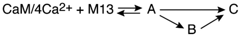
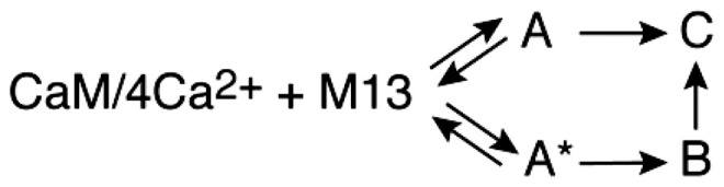
Three models were tested against the DEER-derived time courses by numerical solution of the appropriate differential equations and optimization of the unknown rate constants (Table 2): a linear model (CaM/4Ca²⁺ + peptide $\rightleftharpoons$ A → B → C), a simple branched model (CaM/4Ca²⁺ + peptide $\rightleftharpoons$ A → C and CaM/4Ca²⁺ + peptide $\rightleftharpoons$ A → B → C), and a complex branched model (CaM/4Ca²⁺ + peptide $\rightleftharpoons$ A → C and CaM/4Ca²⁺ + peptide $\rightleftharpoons$ A*→ B → C). In the latter model, states A and A* are both characterized by the 43-Å distance but represent the peptide binding initially to either the CTD or the NTD of CaM (see the next section). Note that the initial bimolecular binding reaction is pseudofirst order under the mixing conditions employed for DEER (a 20-fold excess of M13) (Fig. 2B), and the initial concentration of free CaM/4Ca²⁺ can simply be set to a normalized value of one. Integrated intensities of the 43-, 21-, and 26-Å peaks as a function of t_r are given by I₄₃(t_r) = [A(t_r)] or [A(t_r)] + [A*(t_r)], I₂₁(t_r) = [B(t_r) + (1 – λ)[C], and I₂₆(t_r) = λ[C(t_r)], where λ is also a fitting parameter that determines the ratio of the 21- and 26-Å peak intensities in P(r) for the final complex. Results from the three kinetic models are shown in SI Appendix, Fig. S3. The best fit is obtained with the complex branched model (Fig. 3C, Table 2, and SI Appendix, Fig. S3A).

Table 2.

SDs of global fits to DEER EPR and ssNMR data

Model	SD of fit (%)
	DEER EPR	ssNMR
Linear
	6.3	4.1
Simple branched
	3.4	4.1
Complex branched
	2.3	3.2

The SD of the fit is given by ϕ[RSQ/(d – p)]^1/2, where ϕ is the overall SE of the data, RSQ is the residual sum of squares, d is the total number of experimental points, and p is the number of optimized parameters. Note that RSQ/(d – p) is equivalent to the normalized χ² (i.e., the χ² per degree of freedom). The estimated average value for ϕ is ∼0.025 for the DEER EPR data and ∼0.03 for the ssNMR data.

With the above result in hand, the complete set of DEER echo curves at all T and t_r values was globally fit with the t_r-dependent populations of states A, A*, B, and C calculated from the complex branched kinetic model, yielding excellent fits to the DEER echo curves (SI Appendix, Fig. S4). Excellent agreement was also obtained with populations (Fig. 3 C, Upper Right) and fractional peak intensities (SI Appendix, Fig. S5) obtained from the simpler three-Gaussian global fit. The calculated P(r) distributions from the global four-Gaussian fit for states A/A* at 43 Å, state B at 21 Å, and state C at 21 and 26 Å are shown in Fig. 3D.

Quantitative Analysis of Time-Resolved ssNMR Data.

To obtain a more detailed structural understanding of the A, A*, and B states, we carried out time-resolved ssNMR ¹³C-¹³C correlation experiments that monitor the development of either conformational order (i.e., folding) at residues K5, F8, V11, A13, F17, and I20 of the M13 peptide (Fig. 4A and SI Appendix, Figs. S8 and S9) or intermolecular contacts between methionine methyl groups of CaM and residues F8, A13, and F17 of the M13 peptide (Fig. 4B and SI Appendix, Fig. S10). In the final complex, Met145 is in close proximity to F8, Met71/Met72 to A13, and Met51/Met71 to F17 (8, 10). The time courses of quantities that represent residue-specific conformational order or intermolecular contacts (determined from 2D cross-peak volumes as described in Experimental Procedures) were globally fit to the complex branched model. Under the mixing conditions employed for the ssNMR experiments (1.5 mM CaM/4Ca²⁺ and 2 mM M13), the initial association events to form states A and A* are second order. The normalized time course for each of the nine quantities derived from ssNMR cross-peak volumes is given by Σε_i[X_i(t_r)]/η_i, where [X_i(t_r)] is the concentration of state X_i at time t_r obtained by numerical integration of the differential equations describing the kinetic model and η_i is a normalization factor required because the cross-peak volumes are in arbitrary units. The coefficients ε_i quantify the contribution of each state X_i in the kinetic model to a given ssNMR-derived quantity (as plotted in Fig. 4) relative to state C (i.e., ε_C = 1.0). In other words, the values of ε_i tell us the extent of conformational order or intermolecular interaction that exists for individual isotopically labeled residues of M13 in states A, A*, and B. All nine time courses were fit simultaneously; the rate constants were optimized as global parameters, while the values of ε_i and η_i were optimized for each i.

Fig. 4.

Kinetics of M13 binding to CaM/4Ca²⁺ monitored by time-resolved 2D ssNMR ¹³C-¹³C spectroscopy. (A) Residue-specific time courses for cross-peak signals attributable to the appearance of conformational order within the M13 peptide upon binding to CaM/4Ca²⁺. (B) Residue-specific time courses for cross-peak signals arising from intermolecular contacts between M13 and methionine side chains of CaM. The data in A and B were recorded with spin-diffusion mixing times (τ_SD) of 20 ms and 1 s, respectively; the former generates cross-peaks arising from intramolecular interactions, while the latter generates cross-peaks arising from both intra- and intermolecular interactions. A, Upper and B, Upper show representative 2D spectra of the sample containing ¹³C-[K5,V11,A13,F17]–labeled M13 peptide; the signal intensities are represented by the color scale (shown on the right), which ranges linearly from blue (at a minimum level of ζ that is slightly above the noise) through red (50%) to white (100%). A, Lower and B, Lower show the best fits (continuous lines) to the experimental time courses (circles) using the complex branched binding scheme (Fig. 3C). The experimental normalized intensities as a function of the reaction time t_r were obtained from the 2D spectra as described in detail in Experimental Procedures. The optimized values of the rate constants and the coefficients for the contributions of the various states are provided in Tables 3 and 4, respectively.

An iterative approach was used for optimization of the ε_i coefficients. Initially, coefficients for states A, A*, and B were optimized freely. Subsequently, if the optimized value of a coefficient was found to be very small and was ill defined by the data, its value was set to zero; if a coefficient optimized to a value of greater than one and was poorly defined, its value was set equal to 1.0. Finally, if the coefficient for state A* was greater than that of state B and the 5 to 95% confidence limits of the two coefficients overlapped, the coefficient for state A* was set equal to that of state B during minimization. In addition, the values of ε_i for conformational order at K5 and F8 and at V13 and F17 were set equal as these pairs of experimentally measured quantities are highly correlated (correlation coefficient of 0.995) (Fig. 4A). Although the same is true of the time courses of conformational order at V11 and I20, this constraint on ε_i values was not imposed since V11 and I20 interact with different domains of CaM in the final complex (CTD and NTD, respectively).

The global best fits to the ssNMR experimental data are shown in Fig. 4. As for the DEER data, the ssNMR data fit significantly better to the complex branched scheme than to either the linear or simple branched schemes (Table 2). Optimized values of the rate constants and ε_i coefficients are provided in Tables 3 and 4, respectively. No attempt was made to fit the ssNMR and DEER data together as the experimental conditions were slightly different (e.g., the presence of nitroxide labels for the DEER experiments; pH and salt concentrations, optimized for the two sets of experiments, also differ) (Fig. 2). The values of k_AC, k_A*B, and k_BC are 1.7 (1.2 to 2.3) × 10³, 410 (310 to 540), and 55 (37 to 81) s⁻¹, respectively, slightly smaller than the values determined from the DEER data.

Table 3.

Optimized values of the rate constants for the complex branched kinetic scheme obtained from global fits to the DEER EPR and ssNMR data

	Optimized value (5–95% confidence limits)
	DEER EPR	ssNMR
$k_{on}^A$ (M−1 s−1)	≥5 × 106*	≥5 × 106*
$K_{\text{ass}}^A$ (M−1)	≥5 × 105*	≥4 × 104*
$K_{\text{ass}}^{A*}/K_{\text{ass}}^A$	0.57 (0.48–0.67)	0.56 (0.42–0.74)
kAC (s−1)	≥4 × 103*	1.7 × 103 (1.2 × 103–2.3 × 103)
kA*B (s−1)	660 (570–760)	410 (310–540)
kBC (s−1)	155 (110–215)	55 (37–81)
λ†	0.69 (0.67–0.71)

^*Only lower limits can be determined from both the DEER and ssNMR data for these rate and equilibrium association constants.

^†The ratio of intensities of the 26- to 21-Å distance peaks in the bimodal P(r) distribution for the final complex (state C) is given by λ/(1 − λ).

Table 4.

Optimized values of the relative contributions (ε_i coefficients) to the residue-specific ssNMR time courses from individual states

	Coefficients (5–95% confidence limits)
	State A	State A*	State B	State C
Intramolecular order
K5/F8	0	0	1.0	1.0
V11	0	0	0.5 (0.3–0.8)	1.0
A13/F17	0	0	0	1.0
I20	0	0	0.5 (0.3–0.8)	1.0
Intermolecular contacts
F8	1.0	0	0.6 (0.4–0.9)	1.0
A13	0	0.8 (0.7–1.0)	0.8 (0.7–1.0)	1.0
F17	0	0.4 (0.2–0.6)	0.4 (0.2–0.6)	1.0

An iterative approach was used for the optimization of the ε_i coefficients as described in the text.

An alternative approach to fitting the time-resolved ssNMR data using multiple sets of randomly chosen initial values for fitting parameters and steepest-descent minimizations was also applied independently (Experimental Procedures). This alternative approach yielded optimized rate constants and ε_i values that are consistent with results in Tables 3 and 4. Thus, we consider these conclusions to be robust consequences of the experimental data.

The values of the coefficients ε_i (Table 4) provide structural insight into the nature of the intermediate species, as depicted in Fig. 5. In the final complex, K5 and F8 interact with the CTD of CaM; A13, F17, and I20 interact with the NTD; and V11 interacts with both the NTD and the CTD (8, 10). None of these residues are conformationally ordered (ε = 0) in states A and A*. Thus, the M13 peptide does not acquire its helical secondary structure in the initial association events. In state B, however, K5 and F8 are fully ordered (ε = 1), V11 and I20 are partially ordered (ε ∼ 0.5), and A13 and F17 are disordered (ε = 0). Intermolecular contacts between F8 and methionine side chains of CaM are present in states A (ε ∼ 1) and B (ε ∼ 0.6). For A13 and F17, intermolecular contacts to methionine side chains of CaM are absent in state A but present in states A* and B. While the proximity of A13 to methionine methyls in states A* and B is similar (ε ∼ 0.8) to that in the final complex, contacts between F17 and methionine methyls are more distant or incomplete (ε ∼ 0.4).

Fig. 5.

Kinetic and structural characterization of the complex branched binding pathway for the interaction of M13 with CaM/4Ca²⁺ elucidated by time-resolved DEER and ssNMR. The approximate values for the lifetimes of the various steps are indicated with those derived from the ssNMR data in parentheses. (The optimized values of the rate constants are listed in Table 3.) The initial encounter complexes (states A and A*, the intermediate state B, and the final complex C) are depicted as cartoons; the NTD and CTD of CaM are shown as blue and purple circles, respectively. The M13 peptide is depicted as a ribbon drawing, with the residues monitored by ssNMR indicated by the blue (N-terminal half) and mauve (C-terminal half) spheres.

The simplest explanation of the above data is that the N-terminal half of M13 (which includes F8) contacts the CTD of CaM in state A, while the C-terminal half of M13 (which encompasses V13 and F17) contacts the NTD of CaM in state A*. This interpretation is supported by the fact that the peptide–methionine intermolecular contacts involving F8 are very similar in states A and C (Table 4), and the conversion from state A to state C is fast (Table 3); likewise, the peptide–methionine intermolecular contacts involving V13 and F17 in states A* (open) and B (compact) are very similar (Table 4). However, given that methionines are present in both the NTD and CTD of CaM, one cannot definitively exclude that the M13 peptide binds in reverse in state A* such that its C-terminal half contacts the CTD rather than the NTD, followed by a rearrangement to the correct orientation either in the compact state B or during the final transition from state B to state C. However, this alternative pathway seems physically less likely and would be expected to probably entail an additional intermediate. A further argument against nonnative contacts in state A* involving, for example, alternate methionine residues in the NTD is that the methionine ¹³C_methyl chemical shifts for the intermolecular cross-peaks involving F8, A13, and F17 do not change position or shape as the reaction time increases; nonnative contacts, however, would be expected to produce different cross-peak positions and/or shapes. The ¹³C_methyl chemical shifts for the relevant methionine residues (Met72, Met71 and Met52, and Met145) in the final complex are at 15.5, 19.5, and 21.4 ppm, respectively (23), consistent with the positions of the intermolecular cross-peaks in Fig. 4B and SI Appendix, Fig. S10.

Discussion

The current work demonstrates the combined power of time-resolved DEER and ssNMR to unravel complex kinetic pathways both temporally and structurally. The picture that emerges from global analysis of the combined data for the binding pathway of the intrinsically disordered M13 peptide to the predominantly extended free state of CaM/4Ca²⁺ is one of coupled folding and binding (41, 42) of the peptide, associated with large spatial rearrangements of the two domains of CaM (Fig. 5). The initial steps involve the formation of what can be termed “encounter” complexes, in which either the N-terminal half of M13 binds to the CTD (state A) or the C-terminal half of M13 binds to the NTD (state A*). In states A and A*, the peptide is still intrinsically disordered, and thus, an ensemble of configurations is likely sampled, but in state A, definitive contacts between F8 of M13 and methionine methyl groups of CaM are apparent. States A and A* are largely extended with a mean interspin label distance, r_17R1-128R1, between A17C–R1 on the NTD and A128C–R1 on the CTD of ∼43 Å, slightly reduced from that of the major configuration in the free state (r_17R1-128R1 ∼ 48 Å) (Fig. 3D). The width of the P(r) distribution for states A and A*, however, is broad (∼8 Å) (Fig. 3D and Table 1), indicating that the two domains of CaM sample a wide range of relative orientations with respect to one another. State A undergoes rapid collapse (τ ∼ 0.3 to 0.6 ms) to the final compact state C (r_17R1-128R1 ∼ 21 and 26 Å), presumably because the anchoring of the aromatic ring of F8 in approximately the correct location on the CTD in state A facilitates rapid folding of M13 to an α-helix together with the formation of the correct, “in-register” intermolecular contacts with both the CTD and NTD. Although not monitored in the ssNMR experiments, it seems likely that anchoring of the indole ring of W4 is also important in this regard since the latter makes contact with 12 hydrophobic residues of the CTD in the final complex (8–10). State A* undergoes an approximately five-fold slower conversion (τ ∼ 1.5 to 2.5 ms) to a compact state B (r_17R1-128R1 ∼ 21 Å), in which M13 adopts a partially helical conformation that is more extensive in its N-terminal half than C-terminal half.

The final step from state B to the final complex (state C) is slow (τ ∼ 7 to 18 ms), suggesting that the interactions between the N-terminal half of M13 and the CTD may not be in the correct register in state B. This is supported by calculations of the interspin label P(r) distribution using an R1 rotamer library (Experimental Procedures) based on either the coordinates of the final CaM/4Ca²⁺–M13 complex or a set of modified coordinates in which the first three residues of M13 are deleted. Calculations with full-length M13 yield a bimodal P(r) distribution (SI Appendix, Fig. S6A) that is in excellent agreement with the measured P(r) for state C (Fig. 3D), presumably because of steric constraints imposed by the close proximity of the N-terminal end of the M13 peptide to the nitroxide label at A128C–R1. Calculations with truncated M13 alter the P(r) distribution such that the 21-Å peak becomes the predominant component (SI Appendix, Fig. S6B), in agreement with the P(r) distribution for state B derived from global analysis of the DEER time courses (Fig. 3D). In addition, the $T_{\text{m}}^{\text{app}}$ values for the 21-Å peak, obtained from the global four-Gaussian fit of the DEER data (including their dependence on both T and t_r) (Table 1), are longer for the component attributable to state B than for state C, consistent with closer proximity of the A128C–R1 nitroxide label to protons of M13 in state C. (The $T_{\text{m}}^{\text{app}}$ value for the R1 rotamer corresponding to the 21-Å peak is significantly shorter than that corresponding to the 26-Å peak in state C, which is also fully consistent with the structure and the A128C–R1 rotamer distribution calculated for state C [Table 1 and SI Appendix, Fig. S6A].) One possible explanation is that in the A* to B transition, the N-terminal half of the M13 peptide docks incorrectly onto the NTD such that perhaps W4 occupies the same space that F8 does in the final complex. Indeed, such an out-of-register configuration, which would shift the N-terminal end of the peptide away from A17C–R1 spin label, may account for the slow B to C transition as the peptide threads its way through the staggered clamp created by the two domains of CaM.

An earlier time-resolved ssNMR study by Jeon et al. (23), in which calcium-free CaM was rapidly mixed with a solution containing both M13 and Ca²⁺, found that the N-terminal half of M13 became helical and formed contacts to the CTD of CaM in about 2 ms, while the C-terminal half of M13 became helical and formed contacts to the NTD of CaM in about 8 ms. Comparison with the results described above suggests that binding of Ca²⁺ to the NTD can be a rate-limiting step for completion of the complex if CaM is initially calcium free, consistent with kinetic studies of calcium binding (14), and that the A* branch in Fig. 5 may then be suppressed. However, full kinetic modeling and time-resolved EPR measurements starting with calcium-free CaM have not yet been performed. Additional experiments in which a solution containing calcium-free CaM and M13 is rapidly mixed with Ca²⁺ may also be of interest to test whether weak association of M13 with the CTD of CaM (K_diss ∼ 1 μM, which is about two orders of magnitude weaker than that for the interaction of M13 with CaM/4Ca²⁺), indicated by earlier isothermal titration calorimetry and solution NMR paramagnetic relaxation enhancement measurements (6), affects the process of complex formation.

Concluding Remarks.

The results presented in this paper demonstrate how a combination of time-resolved DEER EPR and ssNMR measurements, combined with global fitting to kinetic models, leads to a detailed understanding of the molecular structural rearrangements underlying the biologically essential process by which calcium-loaded CaM interacts with a target protein. The same approach can be extended to a wide variety of structural conversion processes involved in molecular recognition, protein folding, and assembly, including, for example, the mechanisms whereby proteins on the surface of an enveloped virus engage cell surface receptors to initiate the cascade of conformational transitions that lead to viral entry. Compared with more common techniques, such as time-resolved fluorescence spectroscopy, the magnetic resonance–based approach provides data with much greater structural detail and more direct structural interpretation.

Experimental Procedures

Sample Preparation.

Human CaM was expressed and purified in Escherichia coli BL21(DE3) cells as described previously (6, 23). For ssNMR, CaM was isotopically labeled with ¹³C_methyl-methionine. For DEER measurements, two site-directed mutations at A17C and A128C in the NTD and CTD domains of CaM, respectively, were introduced as sites of attachment for the nitroxide spin labels, and full deuteration was achieved by growing the bacteria in deuterated minimal medium with U-[¹²C/²H]-glucose as the sole carbon source. R1 nitroxide spin labeling was carried out with S-(1-oxyl-2,2,5,5-tetramethyl-2,5-dihydro-1H-pyrrol-3-yl)methyl methanesulfonothioate (Toronto Research Chemicals) as described previously (22, 25).

The 26-residue M13 peptide (KRRWKKNFIAVSAANRFKKISSSGAL) derived from skMLCK was produced synthetically (23). Three different labeling schemes were used. For DEER, the peptide was fully protonated; for ssNMR, one sample was uniformly ¹³C labeled at K5, V11, A13, and F17, and the other was ¹³Cα labeled at A13 and uniformly ¹³C labeled at F8 and I20.

The purity of the protein and peptide samples was verified by mass spectrometry.

Rapid Mixing and Freeze Quenching.

The apparatus used for rapid freezing and mixing was identical to that described previously (21–23). The shortest reaction time that can be achieved with the current apparatus is 1.5 ms. Although a more rapid mixing and freeze-quenching apparatus has recently been reported and demonstrated for DEER measurements with a very impressive dead time of just over 80 μs (24), the sample volumes are too small for ssNMR applications, and the operational time range is less than that of our current setup.

Q-Band DEER.

Pulsed EPR data were collected at Q band (33.8 GHz) and 50 K on a Bruker E-580 spectrometer equipped with a 150-W traveling-wave tube amplifier, a model ER5107D2 resonator, and a cryo-free cooling unit, as described previously (43). Samples were packed in 1.0-mm-inner diameter (1.2-mm-outer diameter) quartz tubes (VitroCom). DEER experiments were acquired using a conventional four-pulse sequence (SI Appendix, Fig. S1A) (44). The observer and electron-electron double resonance (ELDOR) pump pulses were separated by about 90 MHz, with the observer π/2 and π pulses set to 12 and 24 ns, respectively, and the ELDOR π pulse set to 10 ns. The pump frequency was centered at the Q-band nitroxide spectrum located at +40 MHz from the center of the resonator frequency. The τ₁ value of 400 ns for the first echo-period time was incremented eight times in 16-ns steps to average ²H modulation; the position of the ELDOR pump pulse was incremented in steps of Δt = 8 ns. The bandwidth of the overcoupled resonator was 120 MHz. All DEER echo curve were acquired for t_max = 7.5 μs, with the exception of the DEER echo curve for τ₂ < 7.5 μs (T = 15 μs), where t_max was set to the value of τ₂. DEER data were recorded with values of the dipolar evolution time T (=2τ₂) ranging from 2 to 40 μs. Measurement times were approximately as follows: for T = 2 to 10 μs, 3 h; for T = 15 to 25 μs, 12 h; for T = 30 to 35 μs, 36 h; and for T = 40 μs, 72 h.

Q-Band Hahn Spin-Echo Experiment.

Apparent T_m values were measured using a two-pulse Hahn spin-echo experiment with the echo signal recorded as a function of the echo delay time T (SI Appendix, Fig. S1B) (25).

P(r) Distributions and Analysis of T_m-Filtered DEER Series.

P(r) distributions from the DEER echo curves were obtained by model-free validated Tikhonov regularization using the program DeerLab (38) (for example, Fig. 3A) and by a sum of Gaussians to directly fit the experimental DEER data (including background correction with a best-fit exponential decay) using the program DD/GLADDvu (39, 40) (Fig. 3 A and B and SI Appendix, Figs. S2 and S4). Validated Tikhonov regularization was performed with the bootstrap analysis for uncertainty quantification via the bootan function in the DeerLab library, with the number of bootstrap samples evaluated set to 1,000 (38). For global fitting and analysis of the complete second echo period time T (=2τ₂) and reaction times t_r series (Fig. 3B and SI Appendix, Figs. S2 and S4), we imported the fitting routines from DD/GLADDvu (39, 40) into a home-written Python program and included terms that allowed us to treat peak positions and widths as global optimized parameters with and without including a phase memory time T_m dependence of the relative peak intensities as a function of T.

The intensity of a given P(r) peak I_i(T) as a function of T is given by

$$I_i\left(T\right)=p_i\exp \left(-R_{\text{m},i}^{\text{app}}T\right)/{\displaystyle {\sum }_{i=1}^n{p}_i}\exp \left(-R_{\text{m},i}^{\text{app}}T\right),$$ [1]

where $R_{\text{m},i}^{\text{app}}$ is the apparent phase memory time relation rate ($=1/T_{\text{m},i}^{\text{app}}$), p_i is the fractional population of each peak i (at a given reaction time), ${\displaystyle {\sum }_{i=1}^n{p}_i}=1$, and ${\displaystyle {\sum }_{i=1}^n{I}_i}=1$ at every point T. Because there is not sufficient information to determine all the $R_{\text{m}}^{\text{app}}$ values, the $R_{\text{m}}^{\text{app}}$ value for the peak at 26 Å was set to the value of 1/T_m = 0.091 μs⁻¹ obtained from a Hahn spin-echo experiment recorded on the final complex (SI Appendix, Fig. S6). (Note that the exact value of the reference $R_{\text{m}}^{\text{app}}$ does not affect the fits but only impacts the ratios of $R_{\text{m}}^{\text{app}}$ values.) By this means, we are able to determine the fractional populations of the peaks at T = 0, where relative peak intensities are no longer impacted by different values of $R_{\text{m},i}^{\text{app}}$. Minimization was carried out using the least squares Levenberg–Marquard algorithm. In addition, one set of global fit calculations to all the DEER data also incorporated the kinetic scheme for the complex branched binding pathway (Fig. 3C and Table 2), in which the reaction time dependence of the various species was calculated by numerical integration of the corresponding differential equations and the values of the rate constants were optimized (Fig. 3 C, Right and SI Appendix, Figs. S4 and S5).

DNP-Enhanced ssNMR.

Dynamic nuclear polarization (DNP)-enhanced ssNMR measurements were performed at 9.4 T (100.8-MHz ¹³C NMR frequency) and 25 K on a Bruker Avance III spectrometer console, essentially as described previously (23). An extended interaction oscillator (Communications & Power Industries) and quasioptical interferometer (Thomas Keating Ltd.) provided 1.5 W of circularly polarized microwaves at 263.9 GHz. The home-built DNP probe (45) allows for sample cooling to 25 K at MAS frequencies up to 7.00 kHz. For ¹H-¹³C cross-polarization, ¹H and ¹³C radiofrequency (RF) fields of 52 and 45 kHz, respectively, were used with a MAS frequency of 7.00 kHz, and 51- and 46-kHz ¹H and ¹³C RF frequencies, respectively, were used with a MAS frequency of 5.00 kHz. ¹H decoupling was carried out with a ¹H RF field amplitude of 85 kHz using two-pulse phase modulation (46). The 2D ¹³C-¹³C spectra were recorded with a spin-diffusion mixing period τ_SD = 20 ms to look at the appearance of structural order within the M13 peptide and with a spin-diffusion mixing period τ_SD = 1.0 s to observe the appearance of intermolecular contacts (arising from homonuclear dipolar–dipolar interactions) between the residue-specific ¹³C-labeled M13 peptide and ¹³C_methyl-methionines of CaM. The t₁ increment in the indirect dimension was set to 40 μs for the former and 38 μs for the latter [to avoid overlap of the intermolecular ¹³C_aromatic(F8,F17)-¹³C_methyl(Met) cross-peaks with the aliased signals from spinning side bands]; the maximum value of t₁ was 8.0 ms. The recycle delay was set to 1.26 times the buildup time, τ_DNP (typically 3.5 ± 0.5 s), for cross-polarized ¹³C signals under microwave irradiation. Spectra were processed using NMRPipe (47) with 120- to 180-Hz Gaussian line broadening in both dimensions. Contour images of 2D ssNMR spectra were plotted using Igor 6.37 (Wavemetrics, Inc.) from text files generated with the pipe2txt command of NMRpipe, and cross-peak volumes were measured in ImageJ using tiff files generated with the pipe2tiff command of NMRpipe. The 2D ¹³C-¹³C spectra and difference spectra are shown in SI Appendix, Figs. S8–S10.

Normalized intensities plotted in Fig. 4A are [1 – R_a(t_r)], where R_a(t_r) are cross-peak volume ratios that represent fractional populations of conformationally disordered M13 molecules at a residue-specific level. Normalized intensities are then residue-specific fractional populations of conformationally ordered molecules. The cross-peak volume ratios are defined as R_a(t_r) = V_diff(t_r)/V(t_r), where V(t_r) and V_diff(t_r) are cross-peak volumes in the original and difference 2D spectra, respectively. Difference spectra S_diff(t_r) are calculated as S(t_r) – η(t_r)S_∞; S(t_r) and S_∞ are the 2D spectra at reaction time t_r and ∞ (i.e., the final complex), respectively, and η(t_r) is a scale factor adjusted to cancel out the conformationally ordered, helical component of the V11 ¹³C_α/¹³C_β or I20 ¹³C_α/¹³C_γ2,δ cross-peak in S(t_r) (23). ¹³C_α/¹³C_β cross-peak volumes were used to calculate residue-specific R_a(t_r) values for K5, A13, and F17; ¹³C_α/¹³C_β and ¹³C_α/¹³C_γ cross-peak volumes were used for V11, ¹³C_α/¹³C_γ2,δ cross-peaks were used for I20, and ¹³C_α/¹³C_aromatic cross-peaks were used for F8.

Normalized intensities plotted in Fig. 4B are R_b(t_r) = [V_inter(t_r)/V_intra(t_r)]/R_b(∞), where V_intra(t_r) and V_inter(t_r) are volumes of intramolecular M13 cross-peaks and volumes of intermolecular cross-peaks between M13 and methionine methyls of CaM, respectively. For F8 and F17, volumes of intramolecular ¹³C_aromatic/¹³C_β and intermolecular ¹³C_aromatic/¹³C_methyl cross-peaks were used. For A13, volumes of ¹³C_α/¹³C_α diagonal peaks and ¹³C_α/¹³C_methyl cross-peaks were used.

Fitting Time-Resolved DEER and ssNMR Data.

The time courses for the fractional peak intensities and derived species populations from the three-Gaussian global fits to the DEER data were simultaneously fit by nonlinear optimization using the program FACSIMILE (48, 49), which uses a modified Gear method for numerical integration of systems of nonlinear stiff differential equations in conjunction with modified Powell minimization to produce rapid convergence of the sum of squares of residuals for nonlinear systems. The same approach was used for global fitting of the residue-specific time courses derived from ssNMR that describe the appearance of both structural order within the M13 peptide and intermolecular contacts.

A Monte Carlo approach for analysis of the ssNMR-derived quantities plotted in Fig. 4 was also used. The motivation for this approach was to identify all combinations of fitting parameters that produce a reasonably good fit to the ssNMR data (i.e., to identify deep local minima in the deviation between experimental and calculated data). In this approach, initial values of rate constants and ε_i coefficients were chosen randomly (with rate constants between 0.2 and 5.0 times the best-fit values in Table 3 and coefficients between 0.0 and 1.0) and then optimized by steepest-descent minimization of the total χ², defined as ${\displaystyle {\sum }_{j=1}^8{\displaystyle {\sum }_{k=1}^9{\left[E_k\left(t_{r,j}\right)-{\lambda }_k{S}_k\left(t_{r,j}\right)\right]}^2}}/{\sigma }_{kj}^2$, where E_k(t_r,j) and S_k(t_r,j) are experimental and simulated values of quantity k at reaction time t_r,j, σ²_kj is the uncertainty in the experimental value determined from the noise in the 2D ssNMR spectrum, and λ_k is the analytically determined scaling factor that minimizes the contribution to the total χ² from quantity k. In a first set of Monte Carlo analyses, coefficients ε_i (with i = 1, 2, 3, 4 for states A, A*, B, and C, respectively) were constrained by the conditions ε₄ = 1 and ε₂ ≤ ε₃, which correspond to conditions that the maximal conformational order and intermolecular contacts exist in state C and that the extent of conformational order and intermolecular contacts in state A* does not exceed the extent in state B. From 1,000 sets of random initial values, 345 sets of final values with a total χ² < 50 were obtained. Final values of ε₁ and ε₂ were small for quantities that represent residue-specific conformational order at K5, F8, V11, F17, and I20. For quantities that represent conformational order at A13 or intermolecular contacts for F8, A13, and F17, final values of ε₁ and ε₂ covered large ranges. A second set of Monte Carlo analyses was then performed with the additional condition ε₁ε₂ = 0, meaning that either state A or state A* (or both) would not contribute to a given ssNMR-derived quantity. From 1,000 sets of random initial values, 153 sets of minimized values with total χ² < 50 were obtained. Mean values of {ε₁, ε₂, ε₃} for ssNMR-derived quantities that represent conformational order at K5, F8, V11, A13, F17, and I20 were {0.07(0.17), 0.02(0.05), 0.81(0.15)}, {0.04(0.12), 0.01(0.05), 0.90(0.11)}, {0.00(0.03), 0.0(0.0), 0.43(0.14)}, {0.42(0.40), 0.04(0.07), 0.08(0.10)}, {0.01(0.02), 0.01(0.02), 0.14(0.13)}, and {0.01(0.07), 0.0(0.02), 0.54(0.13)}, respectively, with SDs in parentheses. Mean values and SDs for quantities that represent intermolecular contacts for F8, A13, and F17 were {0.52(0.47), 0.13(0.16), 0.65(0.15)}, {0.08(0.27), 0.66(0.20), 0.78(0.04)}, and {0.58(0.49), 0.11(0.14), 0.32(0.14)}, respectively. Thus, the Monte Carlo analysis of the time-resolved ssNMR data supports a near absence of conformational order in states A and A*, nearly full conformational order at K5 and F8 in state B, and partial conformational order at V11 and I20 in state B, as in Table 4. Agreement between experimental and calculated data for F8–CaM contacts was better for parameter sets with the A* coefficient equal to zero (85 of 153 sets, average χ² value equal to 4.51, average A coefficient equal to 0.93) than sets with the A coefficient equal to zero (68 sets, average χ² value equal to 5.12, average A* coefficient equal to 0.30). Agreement between experimental and simulated data for F17–CaM contacts was better for parameter sets with the A coefficient equal to zero (64 of 153 sets, average χ² value equal to 1.86, average A* coefficient equal to 0.26) than sets with the A* coefficient equal to zero (89 sets, average χ² value equal to 2.38, average A coefficient equal to 0.999). For A13–CaM contacts, agreement was better with the A coefficient equal to zero (141 of 153 sets, average χ² value equal to 5.24, average A* coefficient equal to 0.72) than with the A* coefficient equal to zero (12 sets, average χ² value equal to 5.92, average A coefficient equal to 0.998). Thus, the results from the Monte Carlo analysis for intermolecular contacts agree well with those using Powell minimization presented in Table 4.

Calculation of P(r) Distributions from Molecular Coordinates.

P(r) distance distributions between nitroxide spin labels were calculated from molecular coordinates using a rotamer library for the nitroxide spin labels in the program Xplor-NIH (50). P(r) distributions were calculated from existing Protein Data Bank coordinates using a library of R1 residue side-chain conformations whose populations consist of an intrinsic component modulated by overlap with nearby backbone atoms, such that the population of a particular rotamer goes to zero when it closely approaches a backbone atom (SI Appendix has more details). This representation was generated in a fashion analogous to that described by Del Alamo et al. (51).

Data Availability

All study data are included in the article and/or SI Appendix.

References

- 1.Chin D., Means A. R., Calmodulin: A prototypical calcium sensor. Trends Cell Biol. 10, 322–328 (2000). [DOI] [PubMed] [Google Scholar]
- 2.Kuboniwa H., et al. , Solution structure of calcium-free calmodulin. Nat. Struct. Biol. 2, 768–776 (1995). [DOI] [PubMed] [Google Scholar]
- 3.Babu Y. S., et al. , Three-dimensional structure of calmodulin. Nature 315, 37–40 (1985). [DOI] [PubMed] [Google Scholar]
- 4.Baber J. L., Szabo A., Tjandra N., Analysis of slow interdomain motion of macromolecules using NMR relaxation data. J. Am. Chem. Soc. 123, 3953–3959 (2001). [DOI] [PubMed] [Google Scholar]
- 5.Bertini I., et al. , Experimentally exploring the conformational space sampled by domain reorientation in calmodulin. Proc. Natl. Acad. Sci. U.S.A. 101, 6841–6846 (2004). [DOI] [PMC free article] [PubMed] [Google Scholar]
- 6.Anthis N. J., Doucleff M., Clore G. M., Transient, sparsely populated compact states of apo and calcium-loaded calmodulin probed by paramagnetic relaxation enhancement: Interplay of conformational selection and induced fit. J. Am. Chem. Soc. 133, 18966–18974 (2011). [DOI] [PMC free article] [PubMed] [Google Scholar]
- 7.Anthis N. J., Clore G. M., The length of the calmodulin linker determines the extent of transient interdomain association and target affinity. J. Am. Chem. Soc. 135, 9648–9651 (2013). [DOI] [PMC free article] [PubMed] [Google Scholar]
- 8.Ikura M., et al. , Solution structure of a calmodulin-target peptide complex by multidimensional NMR. Science 256, 632–638 (1992). [DOI] [PubMed] [Google Scholar]
- 9.Meador W. E., Means A. R., Quiocho F. A., Target enzyme recognition by calmodulin: 2.4 A structure of a calmodulin-peptide complex. Science 257, 1251–1255 (1992). [DOI] [PubMed] [Google Scholar]
- 10.Clore G. M., Bax A., Ikura M., Gronenborn A. M., Structure of calmodulin-peptide complexes. Curr. Opin. Struct. Biol. 134, 14686–14689 (1993). [Google Scholar]
- 11.Grishaev A., Anthis N. J., Clore G. M., Contrast-matched small-angle X-ray scattering from a heavy-atom-labeled protein in structure determination: Application to a lead-substituted calmodulin-peptide complex. J. Am. Chem. Soc. 134, 14686–14689 (2012). [DOI] [PMC free article] [PubMed] [Google Scholar]
- 12.Kranz J. K., Flynn P. F., Fuentes E. J., Wand A. J., Dissection of the pathway of molecular recognition by calmodulin. Biochemistry 41, 2599–2608 (2002). [DOI] [PubMed] [Google Scholar]
- 13.Frederick K. K., Marlow M. S., Valentine K. G., Wand A. J., Conformational entropy in molecular recognition by proteins. Nature 448, 325–329 (2007). [DOI] [PMC free article] [PubMed] [Google Scholar]
- 14.Park H. Y., et al. , Conformational changes of calmodulin upon Ca2+ binding studied with a microfluidic mixer. Proc. Natl. Acad. Sci. U.S.A. 105, 542–547 (2008). [DOI] [PMC free article] [PubMed] [Google Scholar]
- 15.McMurry J. L., et al. , Rate, affinity and calcium dependence of nitric oxide synthase isoform binding to the primary physiological regulator calmodulin. FEBS J. 278, 4943–4954 (2011). [DOI] [PMC free article] [PubMed] [Google Scholar]
- 16.Yamada Y., Matsuo T., Iwamoto H., Yagi N., A compact intermediate state of calmodulin in the process of target binding. Biochemistry 51, 3963–3970 (2012). [DOI] [PubMed] [Google Scholar]
- 17.Cherepanov A. V., De Vries S., Microsecond freeze-hyperquenching: Development of a new ultrafast micro-mixing and sampling technology and application to enzyme catalysis. Biochim. Biophys. Acta 1656, 1–31 (2004). [DOI] [PubMed] [Google Scholar]
- 18.Mitic S., de Vries S., Rapid Mixing Techniques for the Study of Enzyme Catalysis, Egelman E. H., Ed. (Academic Press, Oxford, United Kingdom, 2012), pp. 514–532. [Google Scholar]
- 19.Pievo R., et al. , A rapid freeze-quench setup for multi-frequency EPR spectroscopy of enzymatic reactions. ChemPhysChem 14, 4094–4101 (2013). [DOI] [PubMed] [Google Scholar]
- 20.Kaufmann R., Yadid I., Goldfarb D., A novel microfluidic rapid freeze-quench device for trapping reactions intermediates for high field EPR analysis. J. Magn. Reson. 230, 220–226 (2013). [DOI] [PubMed] [Google Scholar]
- 21.Jeon J., Thurber K. R., Ghirlando R., Yau W. M., Tycko R., Application of millisecond time-resolved solid state NMR to the kinetics and mechanism of melittin self-assembly. Proc. Natl. Acad. Sci. U.S.A. 116, 16717–16722 (2019). [DOI] [PMC free article] [PubMed] [Google Scholar]
- 22.Schmidt T., Jeon J., Okuno Y., Chiliveri S. C., Clore G. M., Submillisecond freezing permits cryoprotectant-free EPR double electron-electron resonance spectroscopy. ChemPhysChem 21, 1224–1229 (2020). [DOI] [PMC free article] [PubMed] [Google Scholar]
- 23.Jeon J., Yau W. M., Tycko R., Millisecond time-resolved solid-state NMR reveals a two-stage molecular mechanism for formation of complexes between calmodulin and a target peptide from myosin light chain kinase. J. Am. Chem. Soc. 142, 21220–21232 (2020). [DOI] [PMC free article] [PubMed] [Google Scholar]
- 24.Hett T., et al. , Spatiotemporal resolution of conformational changes in biomolecules by combining pulsed electron-electron double resonance spectroscopy with microsecond freeze-hyperquenching. J. Am. Chem. Soc. 143, 6981–6989 (2021). [DOI] [PubMed] [Google Scholar]
- 25.Schmidt T., Clore G. M., Tm filtering by 1H-methyl labeling in a deuterated protein for pulsed double electron-electron resonance EPR. Chem. Commun. (Camb.) 56, 10890–10893 (2020). [DOI] [PMC free article] [PubMed] [Google Scholar]
- 26.Jeschke G., DEER distance measurements on proteins. Annu. Rev. Phys. Chem. 63, 419–446 (2012). [DOI] [PubMed] [Google Scholar]
- 27.Pannier M., Veit S., Godt A., Jeschke G., Spiess H. W., Dead-time free measurement of dipole-dipole interactions between electron spins. J. Magn. Reson. 142, 331–340 (2000). [DOI] [PubMed] [Google Scholar]
- 28.Hubbell W. L., Cafiso D. S., Altenbach C., Identifying conformational changes with site-directed spin labeling. Nat. Struct. Biol. 7, 735–739 (2000). [DOI] [PubMed] [Google Scholar]
- 29.Todd A. P., Cong J., Levinthal F., Levinthal C., Hubbell W. L., Site-directed mutagenesis of colicin E1 provides specific attachment sites for spin labels whose spectra are sensitive to local conformation. Proteins 6, 294–305 (1989). [DOI] [PubMed] [Google Scholar]
- 30.Ward R., et al. , EPR distance measurements in deuterated proteins. J. Magn. Reson. 207, 164–167 (2010). [DOI] [PMC free article] [PubMed] [Google Scholar]
- 31.Schmidt T., Wälti M. A., Baber J. L., Hustedt E. J., Clore G. M., Long distance measurements up to 160 A in the GroEL tetradecamer using Q-band DEER EPR spectroscopy. Angew. Chem. Int. Ed. Engl. 55, 15905–15909 (2016). [DOI] [PMC free article] [PubMed] [Google Scholar]
- 32.Segur J. B., Oberstar H. E., Viscosity of glycerol and its aqueous solutions. Ind. Eng. Chem. 43, 2117–2120 (1951). [Google Scholar]
- 33.Bald W. B., Optimizing the cooling block for the quick freeze method. J. Microsc. 131, 11–23 (1983). [DOI] [PubMed] [Google Scholar]
- 34.Huber M., et al. , Phase memory relaxation times of spin labels in human carbonic anhydrase II: Pulsed EPR to determine spin label location. Biophys. Chem. 94, 245–256 (2001). [DOI] [PubMed] [Google Scholar]
- 35.El Mkami H., Ward R., Bowman A., Owen-Hughes T., Norman D. G., The spatial effect of protein deuteration on nitroxide spin-label relaxation: Implications for EPR distance measurement. J. Magn. Reson. 248, 36–41 (2014). [DOI] [PMC free article] [PubMed] [Google Scholar]
- 36.Baber J. L., Louis J. M., Clore G. M., Dependence of distance distributions derived from double electron-electron resonance pulsed EPR spectroscopy on pulse-sequence time. Angew. Chem. Int. Ed. Engl. 54, 5336–5339 (2015). [DOI] [PMC free article] [PubMed] [Google Scholar]
- 37.Canarie E. R., Jahn S. M., Stoll S., Quantitative structure-based prediction of electron spin decoherence in organic radicals. J. Phys. Chem. Lett. 11, 3396–3400 (2020). [DOI] [PMC free article] [PubMed] [Google Scholar]
- 38.Fábregas Ibáñez L., Jeschke G., Stoll S., DeerLab: A comprehensive software package for analyzing dipolar electron paramagnetic resonance spectroscopy data. Magn. Reson. (Gött.) 1, 209–224 (2020). [DOI] [PMC free article] [PubMed] [Google Scholar]
- 39.Brandon S., Beth A. H., Hustedt E. J., The global analysis of DEER data. J. Magn. Reson. 218, 93–104 (2012). [DOI] [PMC free article] [PubMed] [Google Scholar]
- 40.Hustedt E. J., Stein R. A., Mchaourab H. S., Protein functional dynamics from the rigorous global analysis of DEER data: Conditions, components, and conformations. J. Gen. Physiol. 153, e201711954 (2021). [DOI] [PMC free article] [PubMed] [Google Scholar]
- 41.Sugase K., Dyson H. J., Wright P. E., Mechanism of coupled folding and binding of an intrinsically disordered protein. Nature 447, 1021–1025 (2007). [DOI] [PubMed] [Google Scholar]
- 42.Wright P. E., Dyson H. J., Linking folding and binding. Curr. Opin. Struct. Biol. 19, 31–38 (2009). [DOI] [PMC free article] [PubMed] [Google Scholar]
- 43.Schmidt T., Schwieters C. D., Clore G. M., Spatial domain organization in the HIV-1 reverse transcriptase p66 homodimer precursor probed by double electron-electron resonance EPR. Proc. Natl. Acad. Sci. U.S.A. 116, 17809–17816 (2019). [DOI] [PMC free article] [PubMed] [Google Scholar]
- 44.Pannier M., Veit S., Godt A., Jeschke G., Spiess H. W., Dead-time free measurement of dipole-dipole interactions between electron spins. 2000. J. Magn. Reson. 213, 316–325 (2011). [DOI] [PubMed] [Google Scholar]
- 45.Thurber K. R., Potapov A., Yau W. M., Tycko R., Solid state nuclear magnetic resonance with magic-angle spinning and dynamic nuclear polarization below 25 K. J. Magn. Reson. 226, 100–106 (2013). [DOI] [PMC free article] [PubMed] [Google Scholar]
- 46.Bennet A. E., Rienstra C. M., Auger M., Lakshmi K. V., Griffin R. G., Heteronuclear decoupling in rotating solids. J. Chem. Phys. 103, 6951–6958 (1995). [Google Scholar]
- 47.Delaglio F., et al. , NMRPipe: A multidimensional spectral processing system based on UNIX pipes. J. Biomol. NMR 6, 277–293 (1995). [DOI] [PubMed] [Google Scholar]
- 48.Chance E. M., Curtis A. R., Jones I. P., Kirby C. R., “FACSIMILE: A computer program for flow and chemistry simulations and gereneral initial value problems” in Atomic Energy Research Establishment Report R8775 (H. M. Stationary Office, London, United Kingdom, 1979). [Google Scholar]
- 49.Clore G. M., “Computer analysis of transient kinetic data” in Computing in Biological Science, Geisow M. J., Barrett A. N., Eds. (Elsevier North-Holland, Amsterdam, the Netherlands, 1983), pp. 313–348. [Google Scholar]
- 50.Schwieters C. D., Bermejo G. A., Clore G. M., Xplor-NIH for molecular structure determination from NMR and other data sources. Protein Sci. 27, 26–40 (2018). [DOI] [PMC free article] [PubMed] [Google Scholar]
- 51.Del Alamo D., et al. , Rapid simulation of unprocessed DEER decay data for protein fold prediction. Biophys. J. 118, 366–375 (2020). [DOI] [PMC free article] [PubMed] [Google Scholar]
- 52.Yau W. M., Jeon J., Tycko R., Succinyl-DOTOPA: An effective triradical dopant for low-temperature dynamic nuclear polarization with high solubility in aqueous solvent mixtures at neutral pH. J. Magn. Reson. 311, 106672 (2020). [DOI] [PMC free article] [PubMed] [Google Scholar]
Associated Data
This section collects any data citations, data availability statements, or supplementary materials included in this article.
Supplementary Materials
Data Availability Statement