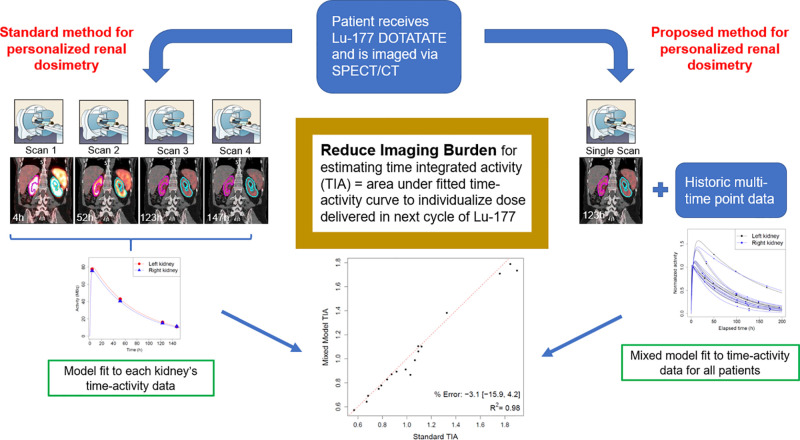
Visual Abstract
Keywords: mixed model, 177Lu-DOTATATE, radionuclide therapy, dosimetry, SPECT/CT
Abstract
Multiple-time-point SPECT/CT imaging for dosimetry is burdensome for patients and lacks statistical efficiency. A novel method for joint kidney time–activity estimation based on a statistical mixed model, a prior cohort of patients with complete time–activity data, and only 1 or 2 imaging points for new patients was compared with previously proposed single-time-point methods in virtual and clinical patient data. Methods: Data were available for 10 patients with neuroendocrine tumors treated with 177Lu-DOTATATE and imaged up to 4 times between days 0 and 7 using SPECT/CT. Mixed models using 1 or 2 time points were evaluated retrospectively in the clinical cohort, using the multiple-time-point fit as the reference. Time–activity data for 250 virtual patients were generated using parameter values from the clinical cohort. Mixed models were fit using 1 (∼96 h) and 2 (4 h, ∼96 h) time points for each virtual patient combined with complete data for the other patients in each dataset. Time-integrated activities (TIAs) calculated from mixed model fits and other reduced-time-point methods were compared with known values. Results: All mixed models and single-time-point methods performed well overall, achieving mean bias < 7% in the virtual cohort. Mixed models exhibited lower bias, greater precision, and substantially fewer outliers than did single-time-point methods. For clinical patients, 1- and 2-time-point mixed models resulted in more accurate TIA estimates for 94% (17/18) and 72% (13/18) of kidneys, respectively. In virtual patients, mixed models resulted in more than a 2-fold reduction in the proportion of kidneys with |bias| > 10% (6% vs. 15%). Conclusion: Mixed models based on a historical cohort of patients with complete time–activity data and new patients with only 1 or 2 SPECT/CT scans demonstrate less bias on average and significantly fewer outliers when estimating kidney TIA, compared with popular reduced-time-point methods. Use of mixed models allows for reduction of the imaging burden while maintaining accuracy, which is crucial for clinical implementation of dosimetry-based treatment.
With recent U.S. Food and Drug Administration approval and ongoing clinical trials for new radionuclide therapies, there is much interest in quantitative imaging for personalized dosimetry-guided treatment. This includes 177Lu-DOTATATE peptide receptor radionuclide therapy (PRRT) for the treatment of neuroendocrine tumors (NETs). Although approved on a fixed-activity basis (7.4 GBq/cycle times 4 cycles), there is much potential to personalize the treatment by exploiting the γ-rays of 177Lu that are suitable for SPECT/CT imaging. SPECT/CT imaging–based dosimetry after 1 cycle can be used to plan the subsequent cycle by safely adjusting the activity based on the renal or renal and lesion absorbed doses (1,2).
Because of the variability in pharmacokinetics, personalized dosimetry in radionuclide therapies typically requires sequential imaging over multiple days after administration to determine the time–activity curve and the area under this curve, known as the time-integrated activity (TIA). Exponential functions are customarily used to fit the measured time–activity data, and 2 or 3 sampling points per exponential term and measurement period up to 3–5 times the effective half-life are recommended (3). Several recent studies have considered simplified personalized renal dosimetry in PRRT (4–12) and 177Lu-PSMA therapy (13,14). In particular, methods for approximating the PRRT TIA using a single activity measurement, introduced for 177Lu-DOTATATE by Hanscheid et al. (4) and for 90Y-DOTATOC by Madsen et al. (5), have gained popularity. Although the approach of individual curve fitting is simple, it is ad hoc for limited sampling points and lacks statistical efficiency because it fails to exploit useful information that may exist across patients. Use of population-level kinetics for all patients may work well for an average patient, but for outliers, large errors are possible. An individual’s time–activity curve may be conceptualized as some deviation from a population-level curve. To personalize treatment, we aim to leverage information across patients while also accounting for individual variation. This formulation naturally lends itself to the mixed modeling approach. Mixed models contain both fixed effects that are shared across all subjects and random effects that vary among patients. Mixed models are commonly used in pharmacokinetics (15), yet application in radionuclide therapy dosimetry has been limited. Previously, our group used nonlinear mixed modeling in 131I radioimmunotherapy to demonstrate good correlation between tracer-predicted and therapy-delivered absorbed doses (16). Merrill et al. (17) used mixed models to create virtual patient time–activity data and estimate both the TIA and the optimal sampling schedule for radioiodine therapy.
To our knowledge, nonlinear mixed models with information sharing, as proposed here, have not been exploited to reduce the imaging burden in radionuclide therapy dosimetry. For 177Lu PRRT of NETs, we constructed biexponential mixed models using complete time–activity data for a historical group of patients and reduced numbers of time points (1 or 2) for new patients. In limited clinical data and in 500 virtual kidneys with realistic pharmacokinetics, we compared the performance of our proposed mixed models with the single-time-point approaches of Madsen et al. (5) and Hanscheid et al. (4). Comparison is also made to standard monoexponential time–activity fitting with 2 time points.
MATERIALS AND METHODS
Patient Characteristics
The clinical study entailed a retrospective analysis of 10 patients (Supplemental Table 1; supplemental materials are available at http://jnm.snmjournals.org) who volunteered for multiple-time-point SPECT/CT imaging after one of the cycles of standard 177Lu-DOTATATE PRRT of NETs performed at the University of Michigan Medical Center between August 2018 and March 2020. The study was approved by the Institutional Review Board, and all patients provided written informed consent.
Patient Imaging and Image Processing
Quantitative Imaging.
Sequential imaging at up to 4 time points (full-time-point data) was performed on a Siemens Intevo Bold SPECT/CT system. For all patients, the first time point was before discharge on the day of therapy, whereas subsequent time points were between days 1 and 7, depending on patient and clinic schedule. An attempt was made to schedule one of these time points at approximately 96 h considering prior reports (4,6) that identified this as optimal for single-time-point imaging–based dosimetry in similar cohorts.
SPECT reconstruction was performed within Siemens xSPECT Quant software using recommended presets (18). Imaging and reconstruction parameters are indicated in Supplemental Table 1. With xSPECT Quant, image voxel values are directly available in units of Bq/mL, hence no external calibration factors were applied.
Kidney Segmentation and Volume-of-Interest (VOI) Propagation
Left and right kidney VOIs were manually segmented slice-by-slice on the CT of the first SPECT/CT image by an experienced technologist. After a contour intensity–based SPECT alignment procedure (19), kidney VOIs were directly propagated to other time points, and time–activity data were extracted.
Standard Biexponential Time–Activity Fit for Clinical Patients
Biexponential models parameterized in Equation 1 were fit to each kidney’s full time–activity data. Although the truth is unknown for patients, we considered this curve and the corresponding TIA as gold standards when evaluating the reduced-time-point methods.
| Eq. 1 |
| Eq. 2 |
Here, scales the curve up or down, (uptake/absorption rate) and (elimination/clearance rate) influence the curve’s shape, and is the measurement error with variance .
Nonlinear Mixed Model Formulation
The mixed model assumes that the parameters , , in Equation 1 can each be expressed as a sum of fixed and random effects. Fixed effects shared across all subjects can be interpreted as population-average values. Random effects represent each subject’s deviation from the mean values. The mixed model was parametrized as:
| Eq. 3 |
Here, represent the fixed effects, and represent the random effects with variances and , respectively. We assume that , , , and are mutually independent. The model specification in Equation 3 implicitly assumes independence between a patient’s 2 kidneys.
The model in Equation 3 is used to fit a biexponential curve to a patient with only 1 or 2 imaging points by jointly fitting this new patient’s limited measurements with full time point data for a prior cohort of patients. With this approach, once multitime point measurements are available for a group of patients to build the mixed model, subsequent patients can be imaged with reduced time points.
Mixed Model Fitting of Clinical Patient Time–Activity Data
Both single-time-point (closest to 96 h) and 2-time-point (∼4 h, closest to 96 h) mixed models were assessed for the clinical patients. Each patient’s time–activity data were artificially reduced to these time points and combined with the full time point data for all other patients to fit the model as shown in Equation 3.
Mixed Model Fitting of Virtual Patient Time–Activity Data
Generating Virtual Patient Kidney Time–Activity
Known time–activity curves for 250 virtual patients (500 kidneys) were generated via a biexponential mixed model based on observed parameter values for the clinical dataset. Random effects were sampled from normal distributions and combined with their respective fixed effects to obtain the kidney-specific parameters. Such parameters were restricted to ranges slightly wider than observed clinical ranges to ensure that simulated data were reflective of the clinical data. Since kidney effective clearance for similar patient cohorts, including outliers, has been reported to be as wide as (35 h, 135 h) (1,4,7,20), the range for was expanded to cover these previously reported ranges. For each virtual patient, 4 time points (full time point data) were selected to reflect the timing in clinical studies. Time point 1 was fixed at 4 h as this is consistent across patients at our clinic, whereas the 3 other time points were allowed to vary with equal probability: time point 2 = {24 h, 36 h, 48 h}; time point 3 = {84 h, 96 h, 108 h}; time point 4 = {144 h, 156 h, 168 h}. Time–activity data for each kidney were normalized to the observed value at time point 1. Measurement error variance after normalization was set to 5% on average at each time point to reflect values reported for 177Lu SPECT/CT quantification with state-of-the-art imaging (18,21,22). This value is consistent with the measurement error used in a prior in silico study of renal time–activity in 177Lu-PSMA therapy (23).
Mixed Model Fitting
For the single-time-point model, we selected time point 3 based on findings that identified approximately 96 h as the optimal single time point (4,6). For the 2-time-point model, in addition to time point 3, time point 1 (4 h) was selected due to the practicality of imaging before a patient is discharged on the day of therapy.
The 250 virtual patients were split into 10 datasets with 25 patients each to facilitate evaluation of our proposed mixed models. For each patient in each dataset, data were reduced down to time point 3 only and time points 1 and 3. Using the reduced data for that patient’s kidneys in combination with the full data of the 24 other patients in the given dataset, mixed models were fit and TIAs were estimated using Equation 3. For the virtual patients, true time–activity curves and TIAs served as gold standards.
Comparison of Reduced-Time-Point Methods
The above single- and 2-time-point mixed models were compared with recently reported single-time-point methods that have been investigated for 177Lu-DOTATATE (4–6,8) as well as a standard monoexponential fit in the case of 2-time-point data. The theoretic, single-time-point approximation of TIA proposed by Madsen et al. (5) assumes prior information is available on population kinetics, whereas the approximation of Hanscheid et al. (4) is based solely on the single activity measurement and the measurement time. For the Madsen method, we investigated monoexponential fit with population mean effective half-life () of 52 h based on previously reported values for similar cohorts (4,6,7) and biexponential Equation 1 approximation with population parameters estimated from the current clinical cohort.
In both clinical and virtual patient data, we compared the gold standard TIAs with TIAs estimated via a biexponential mixed model using 1 time point; a biexponential mixed model using 2 time points; the monoexponential single-time-point Madsen method; the biexponential single-time-point Madsen method; the single-time-point Hanscheid method; and individual monoexponential fit based on 2 time points. For clinical data, the percentage difference between the estimated TIA and the gold standard TIA was calculated. For the virtual data, the percentage bias in the estimated TIA and root mean square error (RMSE) were calculated as measures of accuracy and total error, respectively (24). The goodness of the curve fit was assessed visually and via Pearson R2. All model fitting was done using PROC NLMIXED in SAS version 9.4 (SAS Institute). All other analysis was done in R version 4.0.0 (R Core Team).
RESULTS
Clinical Patient Results
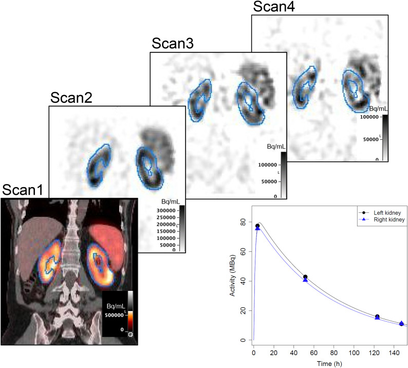
The SPECT alignment and kidney VOI propagation for a typical patient and the corresponding kidney time–activity data are shown in Figure 1. The biexponential individual fits for all clinical cases are shown in Figure 2, with the complete time–activity data and fit parameters given in Supplemental Table 1. The corresponding to had a mean value of 59.6 h (range: 35.4–117.7 h). Because of variations in patient and clinic schedules, there was large variability in all sampling times except for time point 1. For all but 1 case, a measurement close to 96 h (±27 h) was available for our reduced-time-point analysis.
FIGURE 1.
Example (patient 8) images with contour-guided registration showing propagation of kidney contours defined on CT of scan 1 SPECT/CT and corresponding time–activity data with biexponential fits. SPECT images have been normalized to the maximum value in each image.
FIGURE 2.
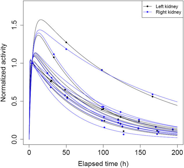
Plot of biexponential time–activity curves and observed data normalized to activity value at first measured time point for all kidneys in clinical patient data.
The reduced-time-point methods applied to the clinical data are compared in Table 1. The single- and 2-time-point mixed models outperform the Madsen or Hanscheid methods for 94% (17/18) and 72% (13/18) of kidneys, respectively. Full- and reduced-time-point fitted curves for 3 example kidneys from the clinical cohort with fast, average, and slow clearance are compared in Figure 3. The mixed model and monoexponential fits for the kidneys with fast (Fig. 3A) and average (Fig. 3B) clearance rates are able to approximate the shape of the gold standard curve quite well. However, for the kidney with slow uptake and clearance rates (Fig. 3C), none of the methods result in fits close to the gold standard curve. The monoexponential fit is essentially horizontal as the first and third time points have approximately equal activity values. The mixed model fits, whereas not close to the gold standard curve, better approximate its shape and TIA.
TABLE 1.
Performance of Reduced-Time-Point (TP) Methods for Clinical Cohort
| % Difference in TIA | |||||||
|---|---|---|---|---|---|---|---|
| Patient | Kidney | Mono 1 TP Madsen | Bi 1 TP Madsen | 1 TP Hanscheid* | 1 TP MM | 2 TP MM | 2 TP Mono |
| 1 | Left | 4.1 [0.88] | −3.1 [0.99] | −3.0 | −1.7 [0.99] | −2.4 [0.99] | −3.1 [0.89] |
| Right | 2.1 [0.88] | −5.0 [0.99] | −4.9 | −3.0 [0.99] | −3.1 [0.99] | −4.0 [0.89] | |
| 2 | Left | 0.7 [0.89] | −4.0 [0.99] | 1.8 | −2.7 0.99] | −0.9 [0.99] | −1.1 [0.90] |
| Right | 0.9 [0.89] | −3.8 [0.99] | 2.0 | −2.5 [0.99] | −0.7 [0.99] | −0.9 [0.90] | |
| 3 | Left | 1.5 [0.93] | −3.3 [0.96] | 2.3 | −1.8 [0.97] | 5.5 [0.98] | 5.4 [0.93] |
| Right | −18.4 [0.92] | −22.3 [0.93] | −17.7 | −15.9 [0.95] | 4.7 [0.98] | 2.6 [0.93] | |
| 4 | Left | −6.2 [0.93] | −10.3 [0.96] | −4.3 | −7.3 [0.97] | −0.5 [0.98] | −1.7 [0.93] |
| Right | −6.9 [0.93] | −11.0 [0.96] | −5.1 | −8.0 [0.97] | −1.2 [0.98] | −2.4 [0.93] | |
| 6 | Left | 0.3 [0.82] | −4.2 [0.97] | 1.7 | −4.4 [0.95] | −6.1 [0.96] | −4.1 [0.85] |
| Right | 2.0 [0.81] | −2.6 [0.97] | 3.4 | −3.0 [0.95] | −4.9 [0.97] | −1.9 [0.84] | |
| 7 | Left | 4.7 [0.90] | 0.2 [0.98] | 6.8 | 0.5 [0.98] | −1.4 [0.99] | 0.7 [0.92] |
| Right | 5.8 [0.87] | 1.2 [0.99] | 7.9 | 1.2 [0.99] | −1.2 [0.99] | 2.3 [0.90] | |
| 8 | Left | 0.7 [0.91] | −6.6 [0.99] | −7.7 | −0.5 [0.99] | 2.8 [0.99] | −0.1 [0.91] |
| Right | −1.4 [0.91] | −8.5 [0.99] | −9.6 | −1.3 [0.99] | 2.6 [0.99] | −0.6 [0.91] | |
| 9 | Left | 9.2 [0.86] | 1.2 [0.99] | 0.0 | 1.1 [0.99] | −2.6 [0.99] | −3.0 [0.88] |
| Right | 15.1 [0.84] | 6.7 [0.99] | 5.4 | 4.2 [0.99] | −1.3 [0.98] | −0.5 [0.87] | |
| 10 | Left | 1.2 [0.64] | −3.1 [0.86] | 3.3 | −2.8 [0.84] | −11.1 [0.98] | 310.7 [0.77] |
| Right | −4.9 [0.62] | −9.0 [0.86] | −2.9 | −8.7 [0.84] | −16.5 [0.97] | 278.0 [0.76] |
Hanscheid approximation provides TIA and not a curve fit.
Patient 5 was excluded from analysis due to not having a ∼96 H measurement. .
MM = mixed model. Mono and Bi refer to monoexponential and biexponential, respectively.
Data in brackets are R2 of curve fit.
FIGURE 3.
Reduced-time-point (TP) fits for patient 3: fast clearance rate (high ke) (A); patient 8: typical clearance rate (average ke) (B); and patient 10: slow clearance rate (low ke) kidneys in clinical cohort (C). Ind = biexponential fit to individual kidney’s time–activity data; MM = mixed model; Mono = monoexponential fit.
Virtual Patient Results
Parameter values used to generate the virtual time–activity data are in Supplemental Table 2. Simulated time–activity curves for right kidneys in 1 representative dataset are shown in Figure 4.
FIGURE 4.
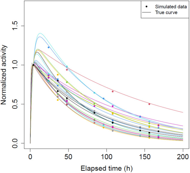
Plot of true time–activity curves and generated 4 time point data normalized to activity value at 4 h for all 25 right kidneys in 1 randomly selected virtual patient dataset.
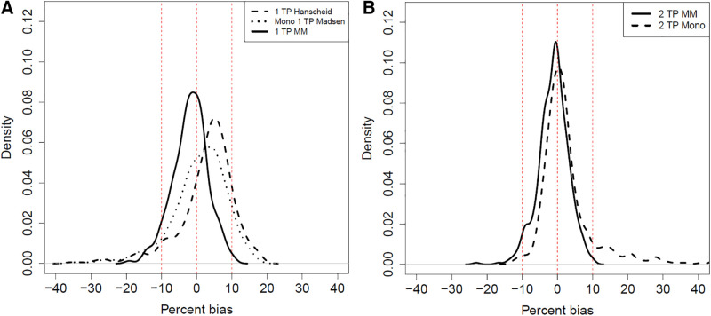
Reduced-time-point methods are compared in Table 2, Figure 5, and Supplemental Figure 1. Mean bias was <7% for all methods. Densities of percentage bias for the mixed models are more concentrated around zero, with less mass in the tails compared with the other methods. RMSE was lowest and R2 highest for the 2-time-point mixed model. Notably, both mixed models exhibited substantially smaller proportions of kidneys with large bias, and the single-time-point mixed model had the narrowest range in bias. For example, 5 (1%) kidneys had mixed model |% bias| > 15% versus 26 (5%) for Madsen and 37 (7%) for Hanscheid. The maximum magnitude of bias was 23% for mixed models, 35% for Madsen, and 36% for Hanscheid.
TABLE 2.
Comparison of Reduced-Time-Point (TP) Methods for Virtual Cohort (500 Kidneys)
| Metric | Mono 1 TP Madsen | Bi 1 TP Madsen | 1 TP Hanscheid | 1 TP MM | 2 TP MM | 2 TP Mono |
|---|---|---|---|---|---|---|
| Mean % bias | 0.7 [−35.1, 17.5] | −3.0 [-38.2, 11.9] | 2.7 [−36.1, 18.5] | −1.9 [−19.2, 10.7] | −1.2 [−23.0, 10.1] | 6.3 [−12.8, 1061.9] |
| # kidneys with |bias| > 10% | 85 (17.0%) | 73 (14.6%) | 102 (20.4%) | 32 (6.4%) | 15 (3.0%) | 70 (14.0%) |
| # kidneys with |bias| > 15% | 26 (5.2%) | 36 (7.2%) | 37 (7.4%) | 5 (1.0%) | 2 (0.4%) | 41 (8.2%) |
| # kidneys with |bias| > 20% | 10 (2.0%) | 18 (3.6%) | 10 (2.0%) | 0 (0.0%) | 1 (0.2%) | 31 (6.2%) |
| # kidneys with |bias| > 25% | 6 (1.2%) | 8 (1.6%) | 8 (1.6%) | 0 (0.0%) | 0 (0.0%) | 21 (4.2%) |
| RMSE | 0.09 | 0.09 | 0.09 | 0.06 | 0.05 | 0.43 |
| Mean R2 of curve fit | 0.87 [0.59, 0.93] | 0.98 [0.82, 0.99] | —* | 0.98 [0.82, 0.99] | 0.99 [0.93, 0.99] | 0.89 [0.74, 0.93] |
Hanscheid approximation provides TIA and not a curve fit.
and
MM = mixed model. Mono and Bi refer to monoexponential and biexponential, respectively. Data in square brackets are minimum and maximum, respectively.
FIGURE 5.
Comparison of percentage bias in TIA for reduced-time-point (TP) methods in virtual cohort of 500 kidneys for 1-time-point methods (A) and 2-time-point methods (B). MM = mixed model. Mono refers to monoexponential fit. One kidney with 2-time-point monoexponential % bias > 1,000 not included in B for visualization purposes.
True curves and reduced-time-point fitted curves for 3 example virtual kidneys with fast, average, and slow clearance rates are compared in Figure 6. The kidneys with fast (Fig. 6A) and average (Fig. 6B) clearance demonstrate that mixed model and individual monoexponential fits can closely approximate the shape of the true activity curve. However, when uptake and clearance are slower than average (Fig. 6C), the monoexponential model results in poor fit. The mixed model fits are also not as accurate as in the other 2 cases but are still closer to the true curves than the monoexponential model.
FIGURE 6.
Reduced-time-point (TP) curve fits, for example, virtual kidneys with fast clearance rate (high ke) (A); typical clearance rate (average ke) (B); and slow clearance rate (low ke) (C). MM = mixed model. Mono refers to monoexponential fit.
DISCUSSION
Statistical mixed models using data from a historical cohort of patients with complete time–activity measurements and subsequent patients with 1 or 2 measurements were constructed and compared with other reduced-time-point methods proposed to obtain TIA for patient-specific dosimetry. All evaluated reduced-time-point methods performed well, with mean |bias| < 7% and < 10% of cases showing |bias| > 15% in a virtual patient study with 500 kidneys (Table 1). However, mixed models substantially reduced the number of outliers, with a 5-fold decrease in the number of virtual kidneys with |bias| > 15%. Mixed models almost always achieved lower bias in the clinical and virtual data and less variability, as demonstrated by the smaller RMSEs for the virtual kidneys. The mixed models effectively eliminated extreme outliers, with 0 of 500 virtual and 0 of 18 clinical kidneys showing bias ≥ 25% in magnitude (Tables 1 and 2).
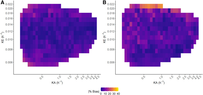
Results from our implementations of the previous single-time-point methods are generally consistent with those reported by Hanscheid et al. (4) and Madsen et al. (5). For a similar patient cohort, using the 96-h time point, Hanscheid et al. (4) reported that 89% (48/54) of kidneys were within 10% of the TIA from multi-time-point imaging, which is consistent with our finding of 80% (398/500; Table 2). Direct comparison with the Madsen method is more difficult as their results were for 90Y-DOTATOC PRRT. However, our finding that for the current application the 96-h single-time-point estimate of Madsen et al. (5) is within 10% of the true estimate for 83%–85% (>415/500) of kidneys (Table 2) is in line with their reported value of 70% at the optimal sampling time of 48 h derived for 90Y-DOTATOC. In general, bias in TIA estimation increases as and move away from their average values, as seen in the heat maps of absolute bias for the virtual patients (Fig. 7, Supplemental Fig. 2). Hanscheid et al. (4) stated that in order for their approximation to achieve < 10% error, the single time point used must be within , . For a monoexponential model, using 96 h as the single time point, this range is equivalent to between (, ). This is consistent with our heat maps for the Hanscheid and Madsen methods, where the largest errors were for high values up to . Note that values below were not observed in the simulations. Mixed models can be viewed through the empiric Bayes framework. Parameter estimates are then shrinkage estimators, meaning that outlier patients and patients with noisy data are drawn closer to the population average than patients whose time–activity curves are more typical or are less noisy. The resulting TIAs may exhibit some small bias but also reduced variance, and thus reduced probability of large bias (Fig. 5). Our clinical analysis was limited by its small sample size, but as more data become available, the results, including outliers (Fig. 3C), should mirror those of the virtual study.
FIGURE 7.
Heat maps of |% bias| vs. biexponential parameters in 500 virtual kidneys for single-time-point mixed model (A) and Hanscheid method (B). White space indicates regions where no kidneys with a specific combination of parameters were simulated.
A limitation of the current study is that we opted to investigate a single measurement at 96 h based on prior reports (4,6). In addition, we chose 4 h as the second time point for patient convenience as it enables imaging before discharge on the day of therapy. For the single time point, Hanscheid et al. (4) discussed the adequacy of an earlier sampling point at 72 h for kidneys where the median effective half-life was 51 h but recommended a later single time point such as 96 or 120 h if considering liver, spleen, and NETs that tend to have longer effective half-lives; reported median effective half-life was 67 h, 68 h, and 77 h, respectively. The theoretic optimal sampling time derived by Madsen et al. (5) was , which for 177Lu-DOTATATE is closest to 72 h for kidney and 120 h for tumor considering the median values reported by Hanscheid et al. (4). Since we aim to pursue mixed modeling for tumor data in the future, we selected 96 h as a compromise, expecting that it would perform well for both kidney and tumor data. This time point is consistent with the recommendations of Hanscheid et al. (4) and Sundlöv et al. For the 2-time-point mixed model, there is potential to consider other combinations of time points that may lead to more accurate estimation of TIA, and others have explored such combinations further, for example in 177Lu-PSMA therapy (13). In our analysis, the single-time-point mixed model often performed better than the 2-time-point mixed model, suggesting that addition of the early measurement may not be necessary. A prior study also suggests that inclusion of a premature activity measure may lead to biased TIA estimates (15). However, inclusion of the initial time point may lead to a better curve fit (R2 > 0.93 vs. > 0.82 in Table 2) compared with using only the approximately 96-h time point. Accurate estimation of the time–activity curve shape can have implications when estimating biologic effective dose where dose rate effects are considered.
Our mixed models were fit assuming kidneys from the same patient and all random effects are independent. Exploring correlation among both kidneys within a patient and among the random effects is an avenue of future work. A potential limitation of our mixed model is the assumption that a historical cohort with multiple-time-point 177Lu SPECT/CT is available, which may not be a reality for many clinics. However, posttreatment SPECT/CT imaging is becoming more accessible with recent updates in reimbursement policies. Furthermore, data sharing across centers, such as the information provided in Supplemental Table 1 and images we have deposited for select patients (patients 4 and 6 in the current study) in the University of Michigan Library Data Sharing repository (25), can facilitate model building.
Although the mixed model demonstrated good performance in our limited clinical cohort and simulations based on this cohort, we expect to validate these results with a larger clinical dataset. With more data, there is also the potential to examine the mixed model’s performance in patient subgroups. For example, separate mixed models could be built based on clinical factors (e.g., estimated glomerular filtration rate, Supplemental Table 1) known to influence kidney pharmacokinetics to further improve fit. Although we limited our investigation to kidney dosimetry after PRRT, it is also possible to extend this method to other therapies and organs. However, validation studies such as the one performed here should be performed for each application before routine clinic use. The most natural extension of our study would be to apply this method to estimating time–activity curves for tumor dosimetry in 177Lu-DOTATATE, and such work in ongoing.
CONCLUSION
This study demonstrates that a mixed model can effectively share time–activity information across patients to improve TIA estimation for patient-specific renal dosimetry relative to other reduced-time-point methods. This novel approach that relies on a historical cohort with complete time–activity data and new patients with 1 or 2 SPECT/CT imaging points resulted in less bias, greater precision, and more than 2-fold and 5-fold reductions in the number of outliers with bias > 10% and > 15%, respectively.
DISCLOSURE
This work was supported by grant R01CA240706, awarded by the National Cancer Institute. No other potential conflict of interest relevant to this article was reported.
KEY POINTS
QUESTION: Can a statistical mixed model based on a historical cohort with complete time–activity data and future patients imaged at only 1 or 2 time points produce accurate TIA estimates for renal dosimetry of patients with NETs treated with 177Lu-DOTATATE?
PERTINENT FINDINGS: The mixed models demonstrated better accuracy and precision in estimating TIA for dosimetry compared with previous reduced-time-point methods that have been investigated for 177Lu PRRT. Most notably, in a virtual study with 500 kidneys, the mixed model reduced the number of outliers with absolute bias in TIA > 10% by more than a factor of 2. In the clinical study, the single-time-point mixed model demonstrated better performance than alternative single-time-point methods in 94% (17/18) of kidneys.
IMPLICATIONS FOR PATIENT CARE: Clinics with access to historical patient time–activity data may reduce imaging for future patients to 1 or 2 time points when performing patient-specific dosimetry. Practical methods that ease the imaging burden to patients and clinics will facilitate clinical implementation of dosimetry-guided radionuclide therapy, which is key to reducing the potential for over- or undertreating patients.
REFERENCES
- 1. Sundlöv A, Sjogreen-Gleisner K, Svensson J, et al. Individualised 177Lu-DOTATATE treatment of neuroendocrine tumours based on kidney dosimetry. Eur J Nucl Med Mol Imaging. 2017;44:1480–1489. [DOI] [PMC free article] [PubMed] [Google Scholar]
- 2. Sandström M, Garske-Román U, Johansson S, Granberg D, Sundin A, Freedman N. Kidney dosimetry during 177Lu-DOTATATE therapy in patients with neuroendocrine tumors: aspects on calculation and tolerance. Acta Oncol. 2018;57:516–521. [DOI] [PubMed] [Google Scholar]
- 3. Siegel JA, Thomas SR, Stubbs JB, et al. MIRD pamphlet no. 16: techniques for quantitative radiopharmaceutical biodistribution data acquisition and analysis for use in human radiation dose estimates. J Nucl Med. 1999;40:37S–61S. [PubMed] [Google Scholar]
- 4. Hänscheid H, Lapa C, Buck AK, Lassmann M, Werner RA. Dose mapping after endoradiotherapy with 177Lu-DOTATATE/DOTATOC by a single measurement after 4 days. J Nucl Med. 2018;59:75–81. [DOI] [PubMed] [Google Scholar]
- 5. Madsen MT, Menda Y, O’Dorisio TM, O’Dorisio MS. Technical note: single time point dose estimate for exponential clearance. Med Phys. 2018;45:2318–2324. [DOI] [PMC free article] [PubMed] [Google Scholar]
- 6. Sundlöv A, Gustafsson J, Brolin G, et al. Feasibility of simplifying renal dosimetry in 177Lu peptide receptor radionuclide therapy. EJNMMI Phys. 2018;5:12. [DOI] [PMC free article] [PubMed] [Google Scholar]
- 7. Willowson KP, Eslick E, Ryu H, Poon A, Bernard EJ, Bailey DL. Feasibility and accuracy of single time point imaging for renal dosimetry following 177Lu-DOTATATE (‘Lutate’) therapy. EJNMMI Phys. 2018;5:33. [DOI] [PMC free article] [PubMed] [Google Scholar]
- 8. Zhao W, Esquinas PL, Frezza A, Hou X, Beauregard JM, Celler A. Accuracy of kidney dosimetry performed using simplified time activity curve modelling methods: a 177Lu-DOTATATE patient study. Phys Med Biol. 2019;64:175006. [DOI] [PubMed] [Google Scholar]
- 9. Guerriero F, Ferrari ME, Botta F, et al. Kidney dosimetry in 177Lu and 90Y peptide receptor radionuclide therapy: influence of image timing, time-activity integration method, and risk factors. BioMed Res Int. 2013;2013:935351. [DOI] [PMC free article] [PubMed] [Google Scholar]
- 10. Heikkonen J, Mäenpää H, Hippeläinen E, Reijonen V, Tenhunen M. Effect of calculation method on kidney dosimetry in 177Lu-octreotate treatment. Acta Oncol. 2016;55:1069–1076. [DOI] [PubMed] [Google Scholar]
- 11. Del Prete M, Arsenault F, Saighi N, et al. Accuracy and reproducibility of simplified QSPECT dosimetry for personalized 177Lu-octreotate PRRT. EJNMMI Phys. 2018;5:25. [DOI] [PMC free article] [PubMed] [Google Scholar]
- 12. Delker A, Ilhan H, Zach C, et al. The influence of early measurements onto the estimated kidney dose in [177Lu][DOTA(0),Tyr(3)]octreotate peptide receptor radiotherapy of neuroendocrine tumors. Mol Imaging Biol. 2015;17:726–734. [DOI] [PubMed] [Google Scholar]
- 13. Rinscheid A, Kletting P, Eiber M, Beer AJ, Glatting G. Influence of sampling schedules on [177Lu]Lu-PSMA dosimetry. EJNMMI Phys. 2020;7:41. [DOI] [PMC free article] [PubMed] [Google Scholar]
- 14. Jackson PA, Hofman MS, Hicks RJ, Scalzo M, Violet JA. Radiation dosimetry in 177Lu-PSMA-617 therapy using a single post-treatment SPECT/CT: a novel methodology to generate time- and tissue-specific dose factors. J Nucl Med. 2020;61:1030–1036. [DOI] [PMC free article] [PubMed] [Google Scholar]
- 15. Davidian M, Giltinan DM. Nonlinear Models for Repeated Measure Data. Chapman and Hall; 1995. [Google Scholar]
- 16. Schipper MJ, Koral KF, Avram AM, Kaminski MS, Dewaraja YK. Prediction of therapy tumor-absorbed dose estimates in I-131 radioimmunotherapy using tracer data via a mixed-model fit to time activity. Cancer Biother Radiopharm. 2012;27:403–411. [DOI] [PMC free article] [PubMed] [Google Scholar]
- 17. Merrill S, Horowitz J, Traino AC, Chipkin SR, Hollot CV, Chait Y. Accuracy and optimal timing of activity measurements in estimating the absorbed dose of radioiodine in the treatment of Graves’ disease. Phys Med Biol. 2011;56:557–571. [DOI] [PubMed] [Google Scholar]
- 18. Tran-Gia J, Lassmann M. Characterization of noise and resolution for quantitative 177Lu SPECT/CT with xSPECT Quant. J Nucl Med. 2019;60:50–59. [DOI] [PubMed] [Google Scholar]
- 19. Mirando D, Dewaraja YK, Cole NM, Nelson AS. In pursuit of fully automated dosimetry: evaluation of an automatic VOI propagation algorithm using contour intensity-based SPECT alignment. Eur J Nucl Med Mol Imaging. 2020;47(suppl 1):S236. [Google Scholar]
- 20. Schuchardt C, Kulkarni H, Zachert C, Baum RP. Dosimetry in Targeted Radionuclide Therapy: the Bad Berka Dose Protocol-Practical Experience. J Postgrad Med. 2013;47:65–73. [Google Scholar]
- 21. Ljungberg M, Celler A, Konijnenberg MW, et al. MIRD pamphlet no. 26: joint EANM/MIRD guidelines for quantitative 177Lu SPECT applied for dosimetry of radiopharmaceutical therapy. J Nucl Med. 2016;57:151–162. [DOI] [PubMed] [Google Scholar]
- 22. Gustafsson J, Brolin G, Cox M, Ljungberg M, Johansson L, Sjögreen Gleisner K. Uncertainty propagation for SPECT/CT-based renal dosimetry in 177Lu peptide receptor radionuclide therapy. Phys Med Biol. 2015;60:8329. [DOI] [PubMed] [Google Scholar]
- 23. Rinscheid A, Kletting P, Eiber M, Beer AJ, Glatting G. Technical note: optimal sampling schedules for kidney dosimetry based on the hybrid planar/SPECT method in 177Lu-PSMA therapy. Med Phys. 2019;46:5861–5866. [DOI] [PubMed] [Google Scholar]
- 24. Casella G, Berger RL. Statistical Inference. Duxbury; 1990: 330. [Google Scholar]
- 25. Dewaraja Y, Van B. Lu-177 DOTATATE anonymized patient datasets: multi-time point Lu-177 SPECT/CT scans [data set], University of Michigan – Deep Blue Data. https://doi.org/10.7302/0n8e-rz46. Published Feb. 20, 2021. Accessed July 12, 2021.


