. 2022 Jan 28;11:e72331. doi: 10.7554/eLife.72331

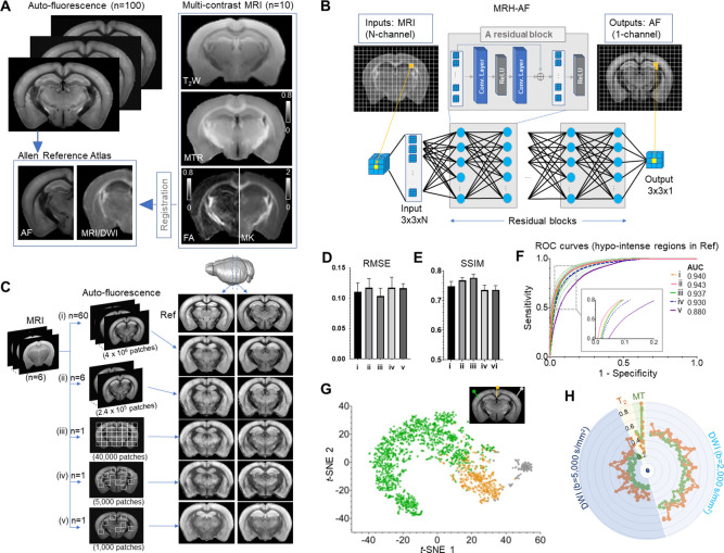
Figure 1. Connect multi-contrast magnetic resonance imaging (MRI) and auto-fluorescence (AF) data of the mouse brain using deep learning.

(A) T2-weighted (T2W), magnetization transfer ratio (MTR), and diffusion-weighted images (DWIs) were registered to the Allen Reference Atlas (ARA) space, from which 100 already registered AF data were selected and down-sampled to the same resolution of the MRI data. Parameter maps derived from DWI, for example, fractional anisotropy (FA) and mean kurtosis (MK), were also included in this study. (B) The deep convolutional neural network (CNN) contained 64 layers (two layers for each residual block × 30 residual blocks plus four additional layers at the input and output ends) and was trained using multiple 3 × 3 MRI patches as inputs and corresponding 3 × 3 patches from histology as targets. (C) The CNN was trained using the MRI data (n = 6) and different amounts of randomly selected AF data (i–v). The results generated by applying the CNN to a separate set of MRI data (n = 4) were shown on the right for visual comparison with the reference (Ref: average AF data from 1675 subject). (D–E) Quantitative evaluation of the results in C with respect to the reference using root mean square error (RMSE) and structural similarity indices (SSIM). The error bars indicate the standard deviations due to random selections of AF data used to train the network. (F) The receiver operating characteristic (ROC) curves of the results in C in identifying hypo-intense structures in the reference and their areas under the curve (AUCs). The ROC curves from 25 separate experiments in (iii) (light green) show the variability with respect to the mean ROC curve (dark green) due to inter-subject variations in AF intensity. (G) The distribution of randomly selected 3 × 3 MRI patches in the network’s two-dimensional (2D) feature space, defined using the t-SNE analysis based on case (iii) in C, shows three clusters of patches based on the intensity of their corresponding patches in the reference AF data (turquoise: hyper-intense, orange: hypo-intense; gray: brain surfaces). (H) MRI signals from two representative patches with hyper-intense AF signals (turquoise) and two patches with hypo-intense AF signals (orange). The orange profiles show higher DWI signals and larger oscillation among them than the turquoise profiles (both at b = 2000 and 5000 s/mm2).

Figure 1.

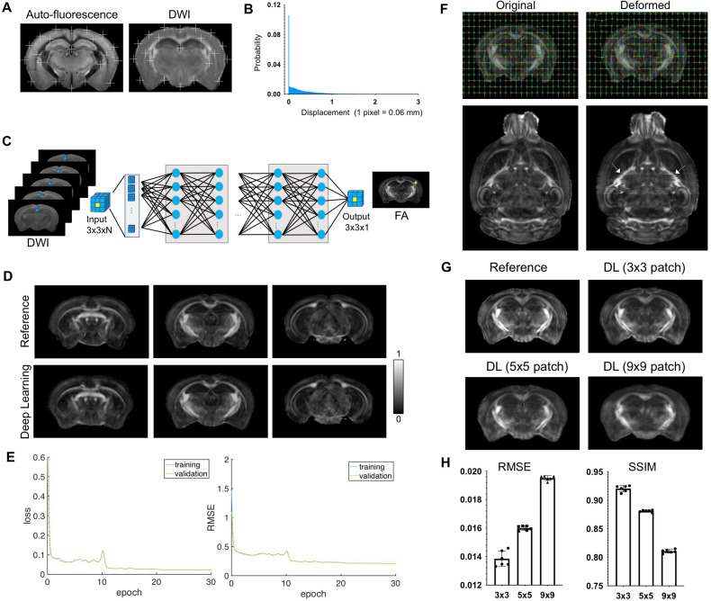
Figure 1—figure supplement 1. Evaluate the effects of mismatches between input magnetic resonance imaging (MRI) data and target auto-fluorescence (AF) data on deep learning outcomes.

Figure 1—figure supplement 1.

(A) The overall registration accuracy was visually examined by overlaying a set of landmarks on AF and average diffusion-weighted (DWI) images. (B) Distribution of pixel displacement due to mismatches between AF and MRI data was estimated using image mapping. Overall, 70% of the pixel displacements are within one pixel (0.0625 mm) and 95% within two pixels (0.125 mm). (C) A convolutional neural network with a similar architecture as the one in the main text was trained using DWIs of ex vivo mouse brains as inputs and corresponding maps of fractional anisotropy (FA), generated by fitting the DWIs to a diffusion tensor model, as targets. In this case, the inputs and targets are perfectly co-registered. (D) Comparisons of FA maps generated from model fitting and from the convolutional neural network (deep learning). Overall, the deep learning results show good agreement with the reference from perfectly registered input and target data. The 3 × 3 patch size used by the network caused smoothing in the deep learning results. (E) Smoothed curves of mean square error loss (left) and root mean square error (RMSE) (right) with respect to the reference FA maps during training measured on the training (blue) and validation (yellow) datasets. Each epoch is 300 iterations. (F) Two-dimensional random displacement fields with the same distribution as shown in A were introduced to deform FA maps in C. The white arrows in the horizontal images indicated the misalignments introduced by this method compared to the original FA maps. Notice the zip-zagged boundaries in the deformed FA map compared to the smooth boundaries in the original FA map. (G) Deep learning results generated using different patch sizes. Larger patch size was able to accommodate more mismatches between input and target data but also increased image smoothing in the results. For the amounts of residual mismatches shown in A, the 3 × 3 patch size was robust to the mismatches with minimal smoothing effects. (H) RMSE and structural similarity index (SSIM) values of results generated using different patch sizes. There were significant differences between different patch sizes (t-test, p < 0.00001).
Figure 1—figure supplement 2. Training convergence curves of MRH auto-fluorescence (MRH-AF) network (A–B) and MRH myelin basic protein (MRH-MBP) during transfer learning.
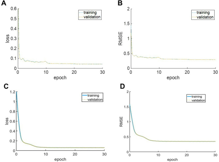
Figure 1—figure supplement 2.

Smoothed curves of mean square error loss (A, C) and root mean square error (RMSE) (B, D) with respect to the reference during training measured on the training (blue) and validation (yellow) datasets. Each epoch is 300 iterations.
Figure 1—figure supplement 3. Evaluation of MRH auto-fluorescence (MRH-AF) results generated using modified 3 × 3 patches with nine voxels assigned the same values as the center voxel as inputs.

Figure 1—figure supplement 3.

(A) Visual inspection showed no apparent differences between results generated using original patches and those using patches with uniform values. (B) Receiver operating characteristic (ROC) analysis showed a slight decrease in area under the curve (AUC) for the MRH-AF results generated using patches with uniform values (dashed purple curve) compared to the original (solid black curve). (C) Correlation between MRH-AF using modified 3 × 3 patches as inputs and reference AF signals (purple open circles) was slightly lower than the original (black open circles).