Impact of mobility on COVID-19 spread – A time series analysis

Abstract

In this paper, we investigate the impact of mobility on the spread of COVID-19 in Tehran, Iran. We have performed a time series analysis between the indicators of public transit use and inter-city trips on the number of infected people. Our results showed a significant relationship between the number of infected people and mobility variables with both short-term and long-term lags. The long-term effect of mobility showed to have a consistent lag correlation with the weekly number of new COVID-19 positive cases. In our statistical analysis, we also investigated key non-transportation variables. For instance, the mandatory use of masks in public transit resulted in observing a 10% decrease in the number of infected people. In addition, the results confirmed that super-spreading events had significant increases in the number of positive cases. We have also assessed the impact of major events and holidays throughout the study period and analyzed the impacts of mobility patterns in those situations. Our analysis shows that holidays without inter-city travel bans have been associated with a 27% increase in the number of weekly positive cases. As such, while holidays decrease transit usage, it can overall negatively affect spread control if proper control measures are not put in place. The result and discussions in this paper can help authorities understand the effects of different strategies and protocols with a pandemic control and choose the most beneficial ones.

Introduction

The recent COVID-19 outbreak is the first global pandemic in the current modern world, and many authorities had no experience dealing with it. Since its confirmation in December 2019 until October 2020 there have been more than 46 million infected cases in the world (WHO, 2019). In Iran, the first confirmed case was reported in February 2020. Since then until October 2020, there have been more than 550,000 reported positive cases, of which over 30,000 cases ended in death. About 83,000 of those infected cases were from Tehran province.

Two major policies that the government used to control the spread of the virus are decreasing the regular outside-the-home daily activities and restrictions on inter-city travels. Such actions are based on the prior knowledge that human mobility is one of the key factors contributing to the spreading of infectious diseases worldwide (Gezairy, 2003), and a strong positive correlation between infectious diseases’ spread and traffic volume is evidenced (Meloni et al., 2009, Wu et al., 2019). Therefore, utilizing mobility data can provide a reliable indicator of the degree of COVID-19′s spread and the effects of pandemic control policies. Also, Kartal et al. (2021) have stated that between some mobility indicators (e.g. trips for grocery, retail, and workplace) and the number of infected people they have witnessed an econometric causality relationship. However, some types of mobility such as walking and driving not seem to have an influence on the pandemic according to Kartal et al. (2021).

There have been many contributions in the literature to study about the impact of COVID-19 on transport system usage and how the pandemic has changed travel patterns (Bhaduri et al., 2020, Lee et al., 2020, Mogaji, 2020, Shamshiripour et al., 2020). Also, there are limited number of studies investigating the effects of mobility on COVID-19. For instance, Hadjidemetriou et al. (2020) examined the effect of government control measures on reducing human mobility and the relationship between the patterns of human mobility and the severe consequences of COVID-19 (e.g. death). Their results demonstrated a significant impact of mobility on the pandemic. In another study, Cartenì et al. (2020) used regression analysis to estimate the effect of different variables on the spread of the virus in Italy. The results showed that mobility habits, environmental variables (such as temperature and pollution), number of tests per day and the proximity to the location of the first outbreak were significant in the model. However, the variable representing mobility habits was the most statistically significant variable explaining the number of COVID-19 cases which indicates the importance of the impact of mobility on the pandemic. The analysis done in Mo et al. (2021) estimated that during their one-month study period on the transit system in Singapore with its highly used and dense transit system, without any control enforcements on public transit system the number of infected people could have increased by 100 times. Therefore, preventive and controlling behaviors are the most effective measures to control the spreading of the epidemic. The impact of mobility on COVID-19′s spread is a complex relationship and various different factors play a part in it. Nevertheless, the studies presented in the literature are limited and have not captured the effects that utilizing the lag that exist between the cause and effect of behavior change or policy on the degree of disease spread. In addition, considering the impact of both inter and intra-city mobility simultaneously and separating the impact of restrictions of each on control the pandemic is yet remained to investigate. To the best of our knowledge, no studies in the literature has considered the gaps presented above, which is the motivation of this study.

In this article, the first objective is to cover the aforementioned gap in the literature. Our main goal is to understand and quantify the impact of inter and intra-city mobility on the number of infected people and the time lag that exists between changes in mobility level and the resulting consequence on the number of new COVID-19 cases. We employed a time-series regression model between the corresponding parameters on a macro-scale level (i.e. City-wide). This modelling is performed based on empirical data from the city of Tehran. The Second objective in our statistical modelling is to investigate the impact of major events and holidays, on the virus spread. Our analysis period includes three important events with significant impacts on the number of infected people: 1) Nowruz Holiday, Persian new-year holiday (March 19-April 1, 2020), 2) Eid al-Fitr (May 23-May 30, 2020) and 3) Ashura (August 8-August 29, 2020). The government utilized different control measures in each of these major events, which led to different mobility patterns and consequently different degrees of disease spread. As such, the lessons learned from different restrictions and control policies can be useful for the authorities.

The rest of this study is organized as follows: Method Section explains the datasets used in this study, how we obtained our model parameters, statistical models employed, and their interpretations. Result and Discussion Section presents a discussion, and finally, Conclusion Section concludes followed by the future research directions.

Method

In this section, first, the datasets used in this study are explained and then developing the time series statistical models are discussed.

Data

We employed different datasets for the time series analysis: COVID-19 positive cases, public transit dataset, and inter-city trips dataset. Each dataset is described in detail in the following next three subsections.

COVID-19 dataset

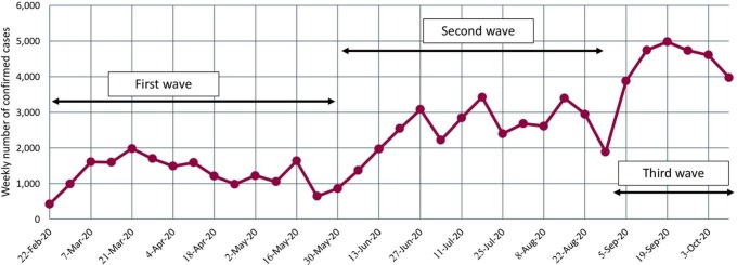
Iran's Ministry of Health’s official data have been used for all COVID-19 related data. We have collected the weekly number of positive cases from February 2019 to October 2020 for Tehran province. In this period, Tehran faced three waves of COVID-19 infection rate (see Fig. 1 ). Mortality from COVID-19 does not only depend on government action and human mobility. It also depends on a variety of other factors such as population density, age, quality of medical treatments and availability of equipment (Docherty et al., 2020, Murthy et al., 2020, Tian et al., 2020). Since considering demographics and quality of medical treatments and availability of equipment are out of the scope of this research, we use the weekly number of infected people as the indicator for virus spread. In addition, the government officials arguably declared that there have been enough test kits in Iran from the beginning of the virus spread (Ministry of Health and Medical Education of Iran) and the unavailability of test kits has not affected the number of positive cases.

Fig. 1.

Weekly COVID-19 cases trend from Feb 2020 to Oct 2020 in Tehran.

Public transit

We collected the AFC (automated fare collection) data of Tehran’s subways and BRTs (Bus Rapid Transit) from January 2019 to October 2020. Around 40% of Tehran’s intra-city travels happen via subway and BRT (Nassereddine and Eskandari, 2017). The data obtained from the AFC system is the temporal and spatial information of the tap-in and tap-out of transit smart cards. The public transportation AFC data consists of smart cards tap-in records for all subway and bus trips and tap-outs for a portion of the subway trips as the tap-out is not mandatory. The dataset also includes the exact time, date, and station of all taps. With the datasets available, we can determine the origin and destination of all trips with tap-out information, and infer the destination and transfer stations on remaining trips based on series of logical, spatial, and temporal rules.

A flowchart (Fig. 2) has been developed for our destination inference algorithm similar to the method proposed in Zhao et al. (2007). We inferred the destination for each trip to create the OD (Origin-Destination) matrix of transit users. For trips consisting of both BRT and subway, we used similar assumptions considered in Nassir et al. (2011) and Gordon et al. (2013). More than 60% of AFC data included only information about entry tap (tap-in) from which 36% are subway only, 43% BRT only, and 21% both; therefore, the algorithm first checks if the tap is related to BRT or subway system. If a trip has a tap-out (for some subway trip records), the destination is known. If there is no tap-out record (for all BRT and some subway trips), the destination is inferred based on the information from the origin of the next trip with the same smart card ID. In the case of inferring the destination of the last trip of the day, the origin of the first trip on the next day is used. Fig. 2 also presents the algorithm for destination inference for trips with a transfer.

Fig. 2.

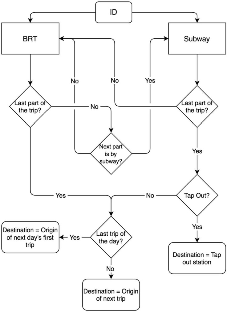
Flowchart of destination inference of mass transit in Tehran from Automated data.

Ridership data alone cannot be a good variable to measure the activity of people in transportation systems during the pandemic. The amount of time or distance traveled in public transit systems can be a better description of people's activity and exposure to the virus in the system. According to the OD matrix inference results, the exact time that each passenger spent in the transportation system could not be calculated, which is due to the lack of Automatic Vehicle Location data. As such, we used the total distance traveled by the passengers per day (daily passenger-kilometer) including both trips with recorded and inferred tap-out stations. This amount is calculated by considering the distance between the location of origin and destination stations.

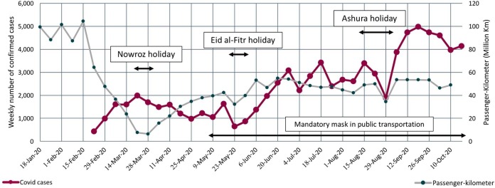
The trend of changes in the estimated passenger-kilometer and the number of infected people is available in Fig. 3 . A significant decline in public transportation ridership happened with the onset of the COVID-19 outbreak. Tehran's public transit experienced an initial 60% drop in its weekly ridership two weeks before Nowruz holiday, and after a few months, settled on around 50% of its pre-pandemic level.

Fig. 3.

Weekly COVID-19 and Passenger-Kilometer trend form Jan 2020 to Oct 2020.

Inter-city trips

We used inter-city travels to capture the effect of traveling in the spread of the disease. According to the reports published by the Statistical Center of Iran (Statistical Center of Iran, 2019), more than 95% of domestic trips in Iran are made by road transportation (e.g. cars and buses). Thus, Tehran province’s traffic counts, extracted from loop detectors placed on all Tehran's inter-province roads from January 2019 to October 2020, were used. 75% of weekly trips to and from Tehran are daily commuting trips from adjacent provinces. The portion of inter-city daily commuters was excluded, because those are part of regular daily work activities and are strongly correlated with the number of transit trips. In addition, the probability of neglecting social distancing and having close contacts with others during recreational trips for trips taking longer than a day are higher than those traveling for daily work and protected by sufficient distancing measures at the workplace.

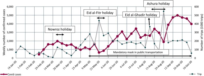
We calculated the difference between the number of entry trips and the number of exit trips of Tehran province for each day as inter-city trip variables for our analysis. As such, it allowed us to neutralize the effect of daily commuters as much as possible. With this logic, if the difference between daily entry and exits is positive, it shows that more people are traveling to the province (visiting trips for non-residents or returning to Tehran by residents). Similarly, if the difference is negative, it shows that more people leaving the province (outside province trips by residents or non-residents leaving the province). Since the study area is Tehran province arrival trips to the province are more relevant. Consequently, we only kept days with a positive number and used the sum of positive numbers for each week as the inter-city trips variable in our analysis. (see Fig. 4)

Fig. 4.

Weekly COVID-19 cases and Number of Trips trend from Jan 2020 to Oct 2020.

Model development

A time-series database was created, consisting of weekly passenger-kilometer data, the number of positive cases of COVID-19, the number of inter-city auto trips (commuters excluded), and two dummy variables for an especial holiday and the period that wearing mask in public transportation system became mandatory. It is worthwhile to note that wearing mask in public places, especially outdoors, did not become mandatory in Tehran. Table 1 presents the list of variables and their definitions in this study.

Table 1.

Description of variables and symbols used in the model.

Variable	Description
$\mathit{INF}$	Weekly number of infected people in unit of 1000 individuals. (dependent variable)
$\mathit{PKM}$	Weekly mass transit passenger-kilometer data in unit of million kilometer.
$\mathit{TRIP}$	Weekly trip data in unit of 1 million vehicles.
${\mathit{INF}}_m$	INF variable with m weeks lag.
${\mathit{PKM}}_{n-m}$	Average of PKM variable from lag n to lag m.
${\mathit{TRIP}}_{n-m}$	Average of TRIP variable from lag n to lag m.
${\mathit{Mask}}_{t-q}$	Binary variable with q weeks lag (is equal to 1 for the weeks that wearing mask was mandatory in public transportation).
${\mathit{Ashura}}_{t-q}$	Binary variable with q weeks lag (is equal to 1 for the three weeks of Ashura ceremonies in Muharram month).

Passengers’ travel patterns may vary according to the day of the week. Therefore, weekly data were used in the model since the periodicity of the data is seven days, meaning that a certain pattern repeats every seven days. Other intervals might not produce uniform data for the model since certain travel patterns may not be taken into account at each interval.

There are other factors such as air pollution and temperature (Cartenì et al., 2020) that can affect the spread of the virus but they were not considered in this study. The absence of certain variables may raise concerns about endogeneity. Technically, endogeneity occurs when there is a correlation between the error term and predictor variable in the model (Weeks, 2002). In that case, the effect of the omitted variable will be considered in the error term. This will result in a violation of one of the OLS assumptions as it will cause a correlation between the independent variables and the error term. In our model that we have omitted some variables, as long as there is no correlation between the included variables and the omitted variables, the omission of variables would not affect the coefficient’s reliability (Greene, 2018). Temperature variable, for instance, is argued to have an effect on the virus spread, but is not correlated with transit use. Thus, omitting the temperature variable in predicting the virus spread would not bias the coefficient of transit use.

Variables and Lags

Due to the silently spreading nature of COVID-19 through communities from those with no symptoms, it is reasonable to investigate the effect of every change in social interaction a few weeks later on the new confirmed COVID-19 cases with signs of COVID-19 and a positive test. Thus, different lags were explored for the variables. The lags are divided into two groups, short-term and long-term. The INF variable is consistent with the mathematical modeling of infectious diseases such as the Susceptible, Infectious, or Recovered (SIR) models (Allen, 1994). The logarithm of INF variable was used in order to prevent negative numbers in the model prediction.

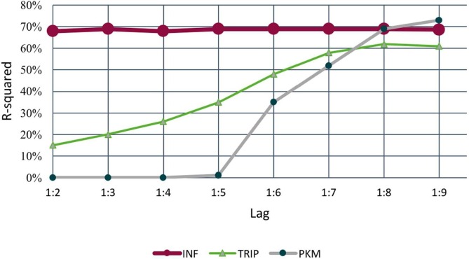
Fig. 5 illustrates the changes of the goodness of fit by adding new lags to each model from 1 to 9 weeks prior to the predicted week. We witnessed no significant changes in goodness-of-fit for INF variable and as the result, the goodness-of-fit seems to be insensitive to the lag variable. The model with the INF with one-week lag is almost well fitted on our observations, which means that this variable gives us enough information about the lagged effect. This trend is consistent with the SIR models.

Fig. 5.

R-squared trends of each variable with different lag ranges.

Public transit usage (PKM) has been used in modeling as one of the parameters that directly affect the incidence rate of COVID-19. According to Fig. 5, the highest amount of goodness of fit belongs to the 1:81 weeks lag. This is because PKM is an indicator of social interactions within the city and it takes more time to see the impact of transit usage on the infection rate. Lags with more than 8 weeks showed no more significant positive effects compared to 6 to 8 weeks lag. Adding further lags reduces the number of observations for training and thereby affects testing statistical models developed. As such, we did not use longer lags to avoid losing more observations. Due to the significant increase in R-squared from model 1:6 onwards, this variable was added to the model in the form of short-term intervals of 1 to 5 weeks lag and long-term intervals of 6 to 8 weeks lag.

The next important mobility variable for the infection rate is the number of inter-city travels. After adding TRIP variable with further lags between 1 and 8 weeks, a significant increase was observed in the R-squared. This variable is discussed more in Variable Interpretation section. To consider the short-term and long-term effects of this variable, it was divided into two separate intervals, consistent with the PKM variable.

We used PKM and TRIP with both lags 1–5 and 6–8, as well as INF with a 1-week lag in our model. For the two dummy variables, Mask and Ashura, after examining different lags, a three-weeks lag results in the best prediction accuracy. Table 2 shows the statistical information of the final variables such as average and average standard error of 32 weeks of observations of each variable.

Table 2.

Statistical information of variables used in model.

	Infected	$\mathit{IN}{F}_1$	$\mathit{PK}{M}_{1-5}$	$\mathit{PK}{M}_{6-8}$	$\mathit{TRI}{P}_{1-5}$	$\mathit{TRI}{P}_{6-8}$	$\mathit{Mas}{k}_{t-3}$	$\mathit{Ashur}{a}_{t-3}$
Unit	1000 Person	1000 Person	1000 Million KM	1000 Million KM	1 Million Vehicle	1 Million Vehicle	Binary	Binary
Number of value	32	32	32	32	32	32	32	32
Min	0.64	0.64	0.02	0.01	0.03	0.03	0.00	0.00
Max	4.98	4.98	0.07	0.10	0.29	0.33	1.00	1.00
Median	2.31	2.10	0.05	0.05	0.19	0.18	1.00	0.00
Mean	2.51	2.43	0.04	0.05	0.18	0.16	0.78	0.09
Average Standard Error	0.22	0.22	0.00	0.00	0.01	0.02	0.07	0.05
Variance	1.61	1.55	0.00	0.00	0.01	0.01	0.18	0.09

Model selection

We used the forward selection approach for the time series multivariable regression analysis in this research which is based on standard OLS (Ordinary Least Squares). A time-series analysis collects data over a period. This method is used to estimate a variable as a function of other parameters over time, called dynamic causality. There are 3 main classes of time-series models: autoregressive models (AR), integrated models (I) and moving average models (MA). By combining these models, some models such as autoregressive moving average models (ARMA) and autoregressive integrated moving average models (ARIMA) were produced (Box et al., 2008). In this study, the model is based on AR model. The dependent variable is modeled along with its lags, as well as some independent variables. Independent variables are added step by step to study the impact of each individual predictor on overall goodness-of-fit.

Table 3 shows the goodness of fit of the model increases as more related variables are added. We began with INF (number of infected people from the previous week). As it could be expected, INF is the predictor with the highest correlation with the dependent variable. As PKM (Model 2) and TRIP (Model 3) variables are added, the model can capture the trend more accurately. In addition, adding dummy variables, Mask (Model 4) and Ashura (Model 5) also increased the goodness of fit of the model. Both of these dummy variables are shown to be statistically significant and increase the prediction accuracy. Wearing mask has been shown very effective in reducing transmission risk in public transportation after it became mandatory. The special event Ashura has also been shown to affect the prediction accuracy. The ceremony takes place around the first three weeks of the lunar month of Muharram (August 15 to September 6). The media coverage during and after these events showed that social distancing was overlooked in lots of gatherings during that time. Also, an increase in the number of infected people in the subsequent weeks could be witnessed from the data that supported those reports. To consider the effect of these gatherings on the infection rate, we added a representing binary variable to the model with a 3-weeks lag, which was shown to have the best fit to the model.

Table 3.

Model development summary for INF as dependent variable.

	Model (1)	Model (2)	Model (3)	Model (4)	Model (5)
(Intercept)	−0.09	−0.43 ***	−0.66*	−1.00 ***	−0.85 ***
	[0.48]	[0.00]	[0.07]	[0.00]	[0.00]
INF1	0.36 ***	0.31 ***	0.67 ***	0.21 ***	0.18 ***
	[0.00]	[0.00]	[0.00]	[0.00]	[0.00]
PKM1–5		9.62 ***	−7.10	−3.11	−3.12
		[0.00]	[0.34]	[0.27]	[0.16]
PKM6–8		1.35	12.30 **	9.47 ***	8.52 ***
		[0.50]	[0.03]	[0.00]	[0.00]
TRIP1–5			5.38 **	5.04 ***	4.02 ***
			[0.02]	[0.00]	[0.00]
TRIP6–8			1.91**	3.47 ***	3.81 ***
			[0.02]	[0.00]	[0.00]
Maskt–3				−0.68 **	−0.59 *
				[0.04]	[0.07]
Ashurat–3					0.35 **
					[0.00]
N. obs.	34	32	32	32	32
R squared	0.69	0.72	0.83	0.88	0.90
Adjusted R squared	0.68	0.69	0.79	0.85	0.87
F statistic	72.41	23.66	24.74	29.35	31.99
P value	0.00	0.00	0.00	0.00	0.00

*** p < 0.01; ** p < 0.05; * p < 0.1.

P-value in brackets.

Our best-fit model is “Model 5” with R-squared being increased from 69% for Model 1 to 90% for Model 5 formulated as below.

$$\text{ln}({\mathit{INF}}_t)\sim {\beta }_0+{\beta }_1{\mathit{INF}}_1+{\beta }_2\mathit{PK}{M}_{1-5}+{\beta }_3\mathit{PK}{M}_{6-8}+{\beta }_4\mathit{TRI}{P}_{1-5}+{\beta }_5\mathit{TRI}{P}_{6-8}+{\beta }_6\mathit{Mas}{k}_{t-3}+{\beta }_7\mathit{Ashur}{a}_{t-3}$$

According to p-values of the best-fit model, except for the $\mathit{PK}{M}_{1-5}$ variable, all other variables are statistically significant. It is important to note that the R-squared value should be interpreted based on the number of observations. According to this, the R-squared value is expected to decrease as the number of observations increases.

To determine whether the model meets the assumptions of the linear regression model, linearity, homoscedasticity, normality, and autocorrelation should be evaluated after the model is developed (Poole and O’Farrell, 1971). These critical assumptions of the ordinary least squares method (OLS) are likely to be violated in a model with limited observations and time-series nature.

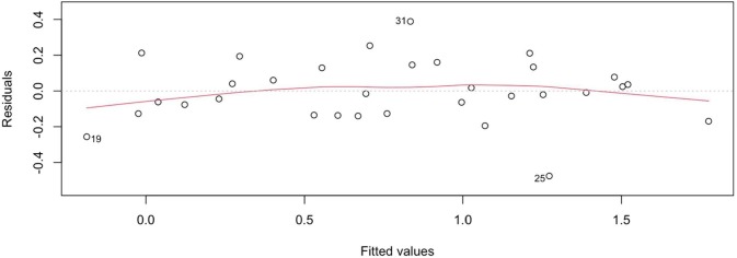
For testing the assumption of linearity, the residuals vs fitted plot are used (see Fig. 6 ). Our linear regression model is linear in parameters, as seen by the equally distributed residuals along a horizontal line with no apparent patterns.

Fig. 6.

Linearity test results.

Breusch-Pagan test (Breusch and Pagan, 1979) is used for checking homoscedasticity on our model's residuals. In this case, the p-value of the test is about 0.86, which indicates that no evidence exists to support the hypothesis that residuals are not homoscedastic (p-value lower than 0.05 would make residuals not homoscedastic).

For the normality test, we use Shapiro-Wilk’s method (Shapiro and Wilk, 1965). The null hypothesis for this test is that the data is normally distributed so if the p-value is significantly close to zero (in this case equal or <0.05), the normality hypothesis will be rejected. The p-value for the Shapiro test for our model's residuals is 0.80 which shows that the normality assumption for model residuals cannot be rejected by the test.

For the potential problem of autocorrelation in our model, the Durbin-Watson statistic is used to investigate the existence of this problem (Savin and White, 1977). The Durbin-Watson test always has a value between 0 and 4. A value of 2.0 evidences no autocorrelation in the residuals. The Durbin-Watson statistic turned out to be 1.85 which is statistically different from 0 and 4 and in a safe range of “no autocorrelation” zone. The Durbin-Watson statistic, however, is slightly below 2 which indicates a tiny tendency toward the positive autocorrelation zone. To make sure this tiny tendency does not affect the standard error of the coefficients, we adopted heteroskedasticity and autocorrelation consistent (HAC) estimators of the variance–covariance matrix (Newey and West, 2014). Although the HAC and classic standard errors are not very different in values, HAC standard errors are used in the model's result as they are more reliable.

Table 4 shows the results of the F-test between models of Table 3 to evaluate whether the increase of goodness of fit is significant. According to Table 3, adding mobility indicator variables (Model 3) increases the goodness of fit by 14%. F-test showed adding these variables resulted in significant improvement to the model. Also, after adding the variable of Mask (Model 4), the R-squared improves to 88%, and the F-test result between Model 3 and Model 4 confirmed that this increase is significant. Finally, comparing Model 5 with Ashura variable added with Model 4, the R-squared increased by 2% and results of the F-test showed this was a significant improvement to the model as well.

Table 4.

F-Test results of comparing models of Table 3.

	F-statics	Degree of Freedom1	Degree of Freedom2	P-value
Model 1 – Model 3	5.35	4	26	0.002
Model 3 – Model 4	10.42	1	25	0.003
Model 4 – Model 5	4.80	1	24	0.038

Result and discussion

In this section, the interpretation of the variables based on the results obtained from our best-fit model, and the stability of model coefficients over different time spans are presented. Furthermore, the impact of some major events during the study period is investigated in order to observe how changes in activity patterns, affect the number of infected people.

Variable interpretation

INF or the number of infected people from the previous week is strongly correlated with the dependent variable, and it could be expected since it was the lag variable. The higher the number of infected people in a week, the more probability of infecting susceptible individuals in the next time step. This observation is consistent with the SIR models as well.

The developed model suggests a strong correlation between PKM and the number of infected people. When the PKM variable is increased by 10 million passenger-kilometers, the number of infected people between one and eight weeks after that will increase by 14.6%. As shown in Fig. 5, this rise does not appear until the fifth week after an increase in the passenger-kilometer rate, and from the sixth to the eighth week, the number of infected people begins to rise and then stabilizes. As discussed earlier, an increase in PKM is an indicator of increased social interaction within the society. This is especially more prominent for public transit usage as social distancing may not be properly followed on busy subway and BRT routes. This observation is consistent with the conclusion in Mo et al. (2021) where they discovered closing the top 40% of high-demand bus routes, which ultimately causes a reduction in demand, can result in a 15.3% reduction in the average number of secondary infections caused by a primary case introduced in a fully susceptible population.

The silently spreading character of the COVID-19 with infected people with no symptoms could be one of the reasons for a relatively long lag (up to 8 weeks) between the PKM variable and the dependent variable. Our model indicates that it takes six to eight weeks until these behaviors show their effect on the number of infected people, which was categorized as long-term effects.

According to the coefficients for TRIP variables in the model, 100,000 increase in TRIP (trips from out of province) leads to a 34.4% increase in weekly cases of infection from one to eight weeks after the increase. According to Fig. 5, the increase takes place gradually up to eight weeks after the TRIP variable was increased, and then it becomes stable. The TRIP variable is to capture the number of the people who were susceptible while traveling to other cities and some became infected during their trip before returning to the province. This causes an increase in the number of positive cases one to five weeks after the trip has ended (short-term impact, TRIP_1-5). Similar to PKM there seems to be a long-term impact between the number of out-of-province trips and the number of infected people 6 to 8 weeks later. The silently spreading nature of COVID-19 from those infected with no symptoms may result in TRIP_6-8 variable being statistically significant. If there are more aggressive testing (without requiring some signs of the disease) such long-term lag for PKM and TRIP may arguably become less statistically significant.

Due to the ignorance of social distancing and health protocols in the ceremonies held in the Ashura holiday, the probability of transmitting the virus from the carriers who participated in these ceremonies is very high. To better capture the effect, a dummy variable (Ashura) was defined in the model. The results of holding this group of ceremonies, based on the model, can be observed in three weeks in terms of infection. Our model indicates that, neglecting all other factors (i.e. mobility indicators), during three weeks of the Ashura event more than 4100 persons became infected with the virus in Tehran province.

Studies have shown that using masks, especially in a public place, can be extremely helpful in reducing the spread of the virus (Eikenberry et al., 2020). In Iran, wearing mask became mandatory in all public transportation vehicles from May 2nd, 2020. We captured the effect of this intervention by introducing a dummy variable in our time series regression analysis. The Mask parameter’s p-value points out a significant impact on the number of infected people (Table 3), and the negative coefficient indicates that it has reduced the number of COVID-19 cases. Based on the Mask variable’s coefficient in the model, after wearing the mask in public transportation become compulsory, it prevented more than 52,900 new COVID-19 cases in the province from May to October 2020.

Stability of coefficients

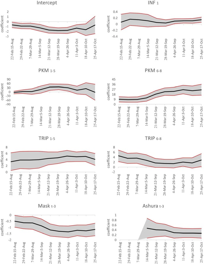
To observe whether regression coefficients are constant during the study period, a stability analysis of all coefficients in different periods was performed. We tested 10 series, each covering 22 consecutive weeks with different start dates, for all model coefficients, as shown in Fig. 7 .

Fig. 7.

Stability of model coefficients with their confidence intervals in different time slots.

The confidence interval for the short-term effect of PKM varies around zero, as the variable is not statistically significant. The model coefficient for long-term PKM seems to jump to a higher value from the end of March 2020. The reason could be due to the fact that after the initial shock to travel patterns at the beginning of the pandemic, people may have gotten used to a new normal travel pattern of using public transit. This observation is also consistent with the transit usage and trends presented in Fig. 1, Fig. 2. The initial lockdown and Nowruz holiday may also affect this model coefficient resulting in a different stable value before the reopening of the economy.

The short-term and long-term effects of the TRIP variable seem to be consistent and do not noticeably change throughout the study period, especially for the short-term effects. It is also observed that the confidence interval of INF decreases as we go forward in time. This may be attributed to the fact that there is more certainty around the true number of confirmed new COVID-19 cases. The same trend happens for Mask as well. It shows that as we go forward in time, more people tend to use masks and it can show its effect better. As for other significant variables, the confidence intervals approximately stay the same throughout all of the series, which shows their coefficients are relatively stable during the study period.

Elasticity values

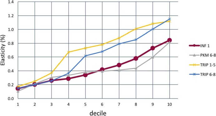
We calculated the elasticity for each of the variable deciles to study their trend changes. For this process, first, the number of deciles for each variable was calculated and then, the average elasticity in each decile was determined.

According to the results in Fig. 8 , The TRIP variable has the highest elasticity growth among all variables and its rate in the ninth and tenth decile reaches more than 1%. This observation shows that a high rate of inter-city travel has a stronger impact on the rate of infection in 1 to 8 weeks later. The rate of elasticity growth in different deciles for the INF and PKM_6-8 variables are similar, which means that every one percent change in these variables causes an approximately equal change in the infection rate.

Fig. 8.

Average elasticity change of variables for each decile.

Impact of especial events

There are three major events throughout our study period: 1) Persian new-year holiday (Nowruz), 2) Eid al-Fitr and 3) Ashura, and each had a significant impact on the number of COVID-19 cases. In the Nowruz holiday, all offices and commercial centers were closed for two weeks and the government put more restrictions on inter-city travel; however, in Eid al-Fitr and Ashura holidays there were no restrictions on inter-city travel as the number of new cases were relatively low at the time.

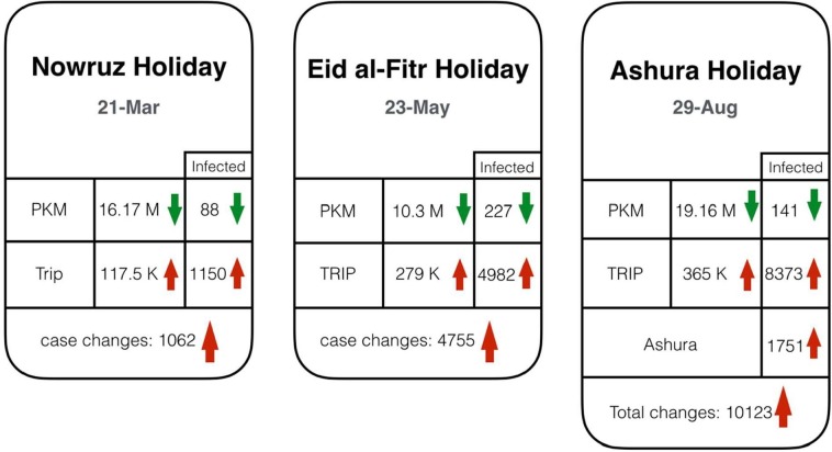
In all three of the holiday periods, we see a decrease in weekly PKM (see Fig. 9). PKM decreased at a higher rate during Nowruz compared with Eid al-Fitr. However, based on our model results, the decrease in the number of new COVID-19 cases caused by the drop in PKM was less during Nowruz because Nowruz was at the very beginning of the pandemic and the total number of cases during that time was significantly lower than Eid al-Fitr, which was during the third peak.

Fig. 9.

Impact of important holidays on the number of infected people.

The increase in the number of inter-city travels has a significant positive effect on the number of infected people in the weeks after. According to Fig. 8, the TRIP variable has the greatest elasticity and effect on increasing the number of new cases. Therefore, holidays without restrictions on inter-city travel not only do not reduce the number of infected people, but also can significantly increase the number of new COVID-19 cases. Lack of restrictions during the Eid al-Fitr and Ashura holidays is the reason that the number of infected people of these two holidays is much higher than the Nowruz holiday.

As it was predicted, due to the holding of ceremonies and the reduction of social distance during the Ashura holiday, the rate of infection is very significant, which is even higher than the number of patients after the Nowruz holiday.

Conclusion

In this paper, our main target was to measure the relationship between the number of new COVID-19 cases and the inter-city and intra-city mobility activities of Tehran. We performed a time-series regression analysis between the indicators of public transit use and of inter-city trips, and other relevant parameters on the number of infected people. For this analysis, transit passenger-kilometer calculated from AFC data was used as the intra-city activity indicator. As for the inter-city mobility indicator, we used the traffic counts in and out of Tehran province excluding commuting trips. The results show that the transit passenger-kilometers variable is statistically significant for the long-term lags (6 to 8 weeks) while the inter-city travel variable is statistically significant for both short-term (1–5 weeks) and long-term. Interestingly, these statistically significant long-term lags exceed the current applied incubation and quarantine periods. This implicates that restrictions and new policies regarding mobility have a much longer lasting impact than the commonly accepted 2–3 weeks period. Thus, a well-adjusted plan for implementing or releasing restrictions for mobility should consider these long-term effects.

We analyzed the impacts of some key events and holidays during the study period. The result from this analysis shows that during holidays, reduced transit usage results in a decrease in the number of new cases. However, if no restriction is in place for out-of-province trips, an increase in the number of them not only will neutralize the positive effect of fewer intra-city mobility, but it possibly can result in an increase in the number of new cases. For instance, during Persian new-year holiday that a travel ban was applied, increase in new COVID-19 was controlled to some extent. However, during the Eid al-Fitr holiday when no restriction on out of province travels were enforced, the negative impact of mobility on new COVID-19 cases were strong. This suggests that governments might need to enforce a set of specific rules and considerations prior to every major event. The ones that are statutory holidays, especially when can be combined with the weekends, usually end up increasing the amount of inter-city trips drastically. Thus, restricting intra-city travel while keeping inter-city travel open could result in a better pandemic control during holidays. On the other hand, holidays during weekdays or observance that include public ceremonies can be controlled through interventions such as nightly traffic curfew.

There were limitations in our study related to data access which can be addressed as possible future directions of this research. We assumed the passenger-kilometer to be the indicator of both mobility and economic activities in the city. However, considering other indicators for economic and social activities (such as bank and credit card transactions separated by transaction types) may help to better separate the impact of mobility on COVID-19. Also, this study was performed with weekly observations. A study with daily intervals can give better and more specific results. Other factors that could also possibly be considered, given data availability, include separation of trip purposes, types and settings of activities outside the home, the infectiousness of the variants in circulation, number of COVID-19 tests per day, weather and climate related factors (e.g. temperature, pollution), spatial components related to exact locations of disease breakout points. Thus, further studies in this matter are encouraged. A comparison of the findings in this paper with other cities can be another interesting area for research.

CRediT authorship contribution statement

Faraz Zargari: Data curation, Formal analysis, Methodology, Software, Investigation, Writing – original draft, Visualization. Nima Aminpour: Data curation, Formal analysis, Methodology, Software, Investigation, Writing – original draft, Visualization. Mohammad Amir Ahmadian: Data curation, Formal analysis, Methodology, Software, Investigation, Writing – original draft, Visualization. Amir Samimi: Conceptualization, Methodology, Validation, Supervision, Resources, Writing – review & editing. Saeid Saidi: Conceptualization, Methodology, Validation, Supervision, Resources, Writing – review & editing.

Declaration of Competing Interest

The authors declare that they have no known competing financial interests or personal relationships that could have appeared to influence the work reported in this paper.

References

- Allen L.J.S. Some discrete-time SI, SIR, and SIS epidemic models. Math. Biosci. 1994;124(1):83–105. doi: 10.1016/0025-5564(94)90025-6. [DOI] [PubMed] [Google Scholar]
- Bhaduri E., Manoj B.S., Wadud Z., Goswami A.K., Choudhury C.F. Modelling the effects of COVID-19 on travel mode choice behaviour in India. Transp. Res. Interdisc. Perspect. 2020;8:100273. doi: 10.1016/j.trip.2020.100273. [DOI] [Google Scholar]
- Breusch T.S., Pagan A.R. A simple test for heteroscedasticity and random coefficient variation. Econometrica. 1979;47(5):1287. doi: 10.2307/1911963. [DOI] [Google Scholar]
- Cartenì A., Di Francesco L., Martino M. How mobility habits influenced the spread of the COVID-19 pandemic: Results from the Italian case study. Sci. Total Environ. 2020;741:140489. doi: 10.1016/j.scitotenv.2020.140489. [DOI] [PMC free article] [PubMed] [Google Scholar]
- Docherty A.B., Harrison E.M., Green C.A., Hardwick H.E., Pius R., Norman L., Holden K.A., Read J.M., Dondelinger F., Carson G., Merson L., Lee J., Plotkin D., Sigfrid L., Halpin S., Jackson C., Gamble C., Horby P.W., Nguyen-Van-Tam J.S., Semple M.G. Features of 20 133 UK patients in hospital with covid-19 using the ISARIC WHO Clinical Characterisation Protocol: Prospective observational cohort study. BMJ. 2020;369(March):1–12. doi: 10.1136/bmj.m1985. [DOI] [PMC free article] [PubMed] [Google Scholar]
- Eikenberry S.E., Mancuso M., Iboi E., Phan T., Eikenberry K., Kuang Y., Kostelich E., Gumel A.B. To mask or not to mask: Modeling the potential for face mask use by the general public to curtail the COVID-19 pandemic. Infect. Dis. Modell. 2020;5:293–308. doi: 10.1016/j.idm.2020.04.001. [DOI] [PMC free article] [PubMed] [Google Scholar]
- Gezairy H.A. Travel epidemiology: WHO perspective. Int. J. Antimicrob. Agents. 2003;21(2):86–88. doi: 10.1016/S0924-8579(02)00365-5. [DOI] [PubMed] [Google Scholar]
- Box G.E.P., Jenkins G.M., Reinsel G.C. 4th ed. Wiley; 2008. Time Series Analysis: Forecasting and Control. [Google Scholar]
- Greene. (2018). Econometric analysis. New York, NY : Pearson; Eighth edition.
- Gordon J.B., Koutsopoulos H.N., Wilson N.H.M., Attanucci J.P. Automated Inference of Linked Transit Journeys in London Using Fare-Transaction and Vehicle Location Data. Transp. Res. Rec. 2013;2343(1):17–24. doi: 10.3141/2343-03. [DOI] [Google Scholar]
- Hadjidemetriou G.M., Sasidharan M., Kouyialis G., Parlikad A.K. The impact of government measures and human mobility trend on COVID-19 related deaths in the UK. Transp. Res. Interdisc Perspect. 2020;6(March) doi: 10.1016/j.trip.2020.100167. [DOI] [PMC free article] [PubMed] [Google Scholar]
- Kartal M.T., Depren Ö., Kilic Depren S. The relationship between mobility and COVID-19 pandemic: Daily evidence from an emerging country by causality analysis. Transp. Res. Interdisc. Perspect. 2021;10(April):1–10. doi: 10.1016/j.trip.2021.100366. [DOI] [PMC free article] [PubMed] [Google Scholar]
- Lee H., Park S.J., Lee G.R., Kim J.E., Lee J.H., Jung Y., Nam E.W. The relationship between trends in COVID-19 prevalence and traffic levels in South Korea. Int. J. Infect. Dis. 2020;96:399–407. doi: 10.1016/j.ijid.2020.05.031. [DOI] [PMC free article] [PubMed] [Google Scholar]
- Meloni S., Arenas A., Moreno Y. Traffic-driven epidemic spreading in finite-size scale-free networks. 2009;106(40):16897–16902. doi: 10.1073/pnas.0907121106. [DOI] [PMC free article] [PubMed] [Google Scholar]
- Mo B., Feng K., Shen Y., Tam C., Li D., Yin Y., Zhao J. Modeling epidemic spreading through public transit using time-varying encounter network. Transp. Res Part C. 2021;122:102893. doi: 10.1016/j.trc.2020.102893. [DOI] [PMC free article] [PubMed] [Google Scholar]
- Mogaji E. Impact of COVID-19 on transportation in Lagos, Nigeria. Transp. Res. Interdisc. Perspect. 2020;6:100154. doi: 10.1016/j.trip.2020.100154. [DOI] [PMC free article] [PubMed] [Google Scholar]
- Murthy S., Gomersall C.D., Fowler R.A. Care for Critically Ill Patients with COVID-19. JAMA. 2020;323(15):1499–1500. doi: 10.1001/jama.2020.3633. [DOI] [PubMed] [Google Scholar]
- Nassereddine M., Eskandari H. An integrated MCDM approach to evaluate public transportation systems in Tehran. Transp. Res. Part A. 2017;106(August):427–439. doi: 10.1016/j.tra.2017.10.013. [DOI] [Google Scholar]
- Nassir N., Khani A., Lee S.G., Noh H., Hickman M. Transit Stop-Level Origin–Destination Estimation through Use of Transit Schedule and Automated Data Collection System. Transp. Res. Rec. 2011;2263(1):140–150. doi: 10.3141/2263-16. [DOI] [Google Scholar]
- Newey W., West K. A simple, positive semi-definite, heteroscedasticity and autocorrelation consistent covariance matrix. Appl. Econometr. 2014;33(1):125–132. doi: 10.2307/1913610. [DOI] [Google Scholar]
- Official: Iran ready to export COVID-19 test kits to regional states. (n.d.).
- Poole M.A., O’Farrell P.N. The assumptions of the linear regression model. Trans. Inst. Br. Geogr. 1971;52(52):145. doi: 10.2307/621706. [DOI] [Google Scholar]
- Savin N.E., White K.J. The Durbin-Watson test for serial correlation with extreme sample sizes or many regressors. Econometrica. 1977;45(8):1989. doi: 10.2307/1914122. [DOI] [Google Scholar]
- Shamshiripour, A., Rahimi, E., Shabanpour, R., & Mohammadian, A. (Kouros)., 2020. How is COVID-19 reshaping activity-travel behavior? Evidence from a comprehensive survey in Chicago. Transp. Res. Interdiscip. Perspect., 7, 100216. https://doi.org/10.1016/j.trip.2020.100216. [DOI] [PMC free article] [PubMed]
- Shapiro S.S., Wilk M.B. An Analysis of Variance Test for Normality (Complete Samples) Biometrika. 1965;52(3-4):591–611. doi: 10.1093/biomet/52.3-4.591. [DOI] [Google Scholar]
- Statistical Center of Iran > Home. (n.d.).
- Tian J., Yuan X., Xiao J., Zhong Q., Yang C., Liu B., Cai Y., Lu Z., Wang J., Wang Y., Liu S., Cheng B., Wang J., Zhang M., Wang L., Niu S., Yao Z., Deng X., Zhou F., Wei W., Li Q., Chen X., Chen W., Yang Q., Wu S., Fan J., Shu B., Hu Z., Wang S., Yang X.-P., Liu W., Miao X., Wang Z. Clinical characteristics and risk factors associated with COVID-19 disease severity in patients with cancer in Wuhan, China: a multicentre, retrospective, cohort study. Lancet Oncol. 2020;21(7):893–903. doi: 10.1016/S1470-2045(20)30309-0. [DOI] [PMC free article] [PubMed] [Google Scholar]
- Weeks, M., 2002. Book Reviews : Introductory Econometrics: A Modern Approach, Jeffrey M. Wooldridge, South-Western College Publishing, 2000, 1-538-85013-2, 824. J. Appl. Econ., 17(2), 191–193. https://doi.org/10.1002/jae.665.
- WHO Coronavirus Disease (COVID-19) Dashboard | WHO Coronavirus Disease (COVID-19) Dashboard. (n.d.).
- Wu Y., Pu C., Li L., Zhang G. Traffic-driven epidemic spreading and its control strategies. Digital Commun. Netw. 2019;5(1):56–61. doi: 10.1016/j.dcan.2018.10.005. [DOI] [Google Scholar]
- Zhao Jinhua, Adam Rahbee, Nigel HM Wilson. Estimating a rail passenger trip origin‐destination matrix using automatic data collection systems. Comput.‐Aided Civ. Inf. Eng. 2007;22(5):376–387. [Google Scholar]