Abstract
In the process of coal mining, a certain amount of gas will be produced. Environmental perception is very important to realize intelligent and unmanned coal mine production and operation and to reduce the accident rate of gas explosion and other disasters. The identification of geometric features of the coal mine working face is the main part of the environmental perception of the working face. In this study, we identify geometric features in a large-scale coal mine working face point cloud (we take the ball as an example) so as to provide a method for the environmental perception of the coal mine working face. On the basis of previous research, we upgrade the dynamic graph convolution neural network (DGCNN) for directly processing point clouds from two aspects: extracting local features and global features of point clouds. First, a multiscale dynamic graph convolution neural network (MS-DGCNN) is proposed, and the combination of max-pooling and average-pooling is used as the symmetry function. Second, we use MS-DGCNN to learn the features of a variety of geometric point clouds in the point cloud data set we make and then look for the ball in the large-scale point cloud of the coal mining working face. Finally, we compare the performance of MS-DGCNN with that of other deep neural networks directly processing point clouds. This study enables MS-DGCNN to obtain more powerful feature expression ability and enhance the generalization of the model. In addition, this study provides a solid foundation for the geometric feature identification of MS-DGCNN in the environmental perception of the coal mine working face and creates a precedent for the application of MS-DGCNN in the field of energy. At the same time, this study makes a beneficial exploration for the development of a transparent coal mine working face.
1. Introduction
Coal is an important basic energy and raw material.1 As the core technical support to realize the high-quality development of the coal industry, intelligent coal mining is the development direction and inevitable trend of safe and efficient coal mining, which has become an industry consensus.2,3 Intelligent coal mining is the deep integration of equipment and technologies, such as artificial intelligence, big data, and robots with coal mine working face to form an intelligent mining system with comprehensive perception, autonomous learning, and collaborative control.4,5 The coal mine working face is one of the most complex places for the coal mining operation. It should be noted that to realize the high intelligence of the coal mine working face, it is necessary to be based on environmental perception.6−8 Environmental perception is an indispensable part for the development of an intelligent coal mine working face.
The identification of geometric features of coal mine working face is a necessary part of the environmental perception of the coal mine working face. The realization of the identification of target feature in the coal mine working face can provide data basis for intelligent decision-making and control of mining equipment.9,10 In this study, we have used our proposed method to perceive and recognize the target features in the point cloud of the coal mine working face (we take the ball in the coal mine working face as an example) so as to provide an effective method for the environmental perception of the actual coal mine working face. This method has strong generalization and universality and can provide the premise and basis for identifying a variety of geometric features and more complex geometric features. For example, the subsequent extension of this method is to identify each hydraulic support in the point cloud of coal mine working face, which can provide a basis for adaptive straightening of the coal mine working face.
The existing method of environmental perception in coal mine working face is the machine vision method. The machine vision method uses multiple cameras to collect the images of the coal mining environment and realizes the environmental perception in coal mine working face through relevant image processing algorithms.11,12 This method has the advantages of a large measurement range, a large amount of information, and a low cost. However, due to the low illumination and large dust in the coal mine working face, the image quality is affected and the measurement effect depends on the position and number of cameras, which affects the measurement accuracy and stability. Furthermore, machine vision is mainly used in occasions with low real-time requirements. Subject to the hardware processing speed and the error of visual measurement, the machine vision method has certain limitations for the environmental perception in coal mine working face.13,14
Another method is the ultra-wide-band method, which transmits data through nanosecond to microsecond non-sine wave narrow pulses, which can realize the detection of targets in the coal mine working face. It has the advantages of a fast transmission speed and a low power consumption.15,16 However, in the coal mine working face, due to the high equipment density, the reflection, refraction, and diffraction of the metal surface on the pulse signal are serious, resulting in a low refresh rate and increased power consumption, which affects the range and accuracy of ultra-wide-band sensing.17,18
The inertial navigation method is a completely autonomous sensing system. It relies on gyroscopes and accelerometers and uses the track estimation algorithm of integral operation to continuously provide a variety of parameters such as the azimuth of fully mechanized mining equipment.19 However, the inertial navigation method involves integral operation, and the error will gradually increase with time. It is not suitable for fully mechanized mining equipment with a low speed and high vibration, and its long-time work will produce a large accumulated error. In addition, the initialization time is long when the inertial navigation system is started.20,21
Due to the fluctuation of coal seams in the working face, the changeable geological environment, the influence of water mist, and electromagnetic interference in the workplace, a variety of perception means cannot be applied. At present, there are still many difficulties in the accurate perception of the mining environment of the coal mine working face. It is an urgent need to find out an effective and reliable perception means that can adapt to the special mining process in the coal mine working face.22−26 Laser has characteristics of strong dust penetration, good unidirectionality, and strong anti-interference ability.27,28 Therefore, we collect the point cloud of the whole coal mine working face by LiDAR to characterize the mining environment of the working face. Furthermore, the expression of point cloud is simpler. Any geometric feature in the point cloud of the coal mining face can be expressed as an N*D matrix. Most importantly, point cloud has three-dimensional coordinates compared with images, which can better and more accurately express the spatial attribute relationship of environmental elements, such as coal wall, underground fully mechanized mining equipment, and so on.
At present, the point cloud feature extraction methods based on the deep neural network can be mainly divided into three categories: multiview method, voxelization method, and direct point cloud processing method.29,30 However, the multiview method changes the local and global structures of the point cloud in the transformation process, which reduces the feature discrimination.31 In the voxelization method, to avoid voxels occupying a lot of storage space, resulting in high computing and memory requirements, the resolution of three-dimensional voxels cannot be too high, so the expression of point cloud data will be lost, and it is difficult to extract the fine-grained features of the point cloud.32 PointNet, directly processing the point cloud, breaks through the bottleneck of deep neural network to process the point cloud, but PointNet is so independent to process each point in the point cloud that it ignores the relevant information between points, resulting in the loss of part of the local feature information of the point cloud.33 By comparison, DGCNN can directly take the point cloud as the input, which uses the edge convolution operation to extract the features of the center point and the edge vectors of K points near the center point to obtain the local features of the point cloud.34,35
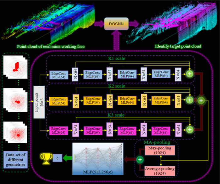
However, some of the local feature areas of the working face point cloud extracted by single-scale edge convolution in DGCNN will be missing or redundant, which affects the geometric feature extraction effect of DGCNN on the working face point cloud. Besides, DGCNN takes max-pooling as a symmetric function to extract the global features of the point cloud.36,37 Although this operation can ensure the disorder of the point cloud, it lacks the information of all points except the point with the largest eigenvalue in the point cloud. Therefore, based on the previously established DGCNN model, we proposed MS-DGCNN to extract the local features of point clouds. This can not only solve the problems of single-scale edge convolution, but also multiscale edge convolution uses different scales to build dynamic local neighborhoods and splice the features extracted at different scales, which learns the local features of point cloud at a deeper and more level. It is remarkable because average-pooling is an operation considering the features of all points in the point cloud, so we have added average-pooling as the symmetric function of MS-DGCNN to extract the global features of the point cloud on the basis of the max-pooling, which can not only ensure the disorder of the point cloud but also can effectively solve the problem of global information loss caused by the max-pooling in DGCNN.
We have used MS-DGCNN to find the target (ball) in the point cloud of coal mine working face, which not only provides a solid foundation for the geometric feature identification in the coal mine working face environmental perception but also makes a beneficial exploration for promoting the development of transparent coal mine working face. Apparently, this study innovates the research method of coal mine working face environmental perception and creates a precedent for the application of MS-DGCNN in the field of energy.
2. Materials and Methods
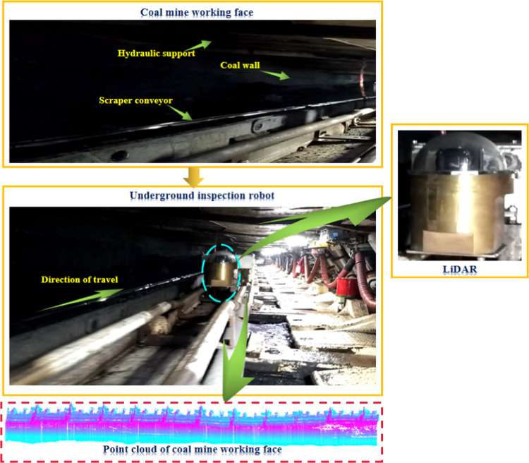
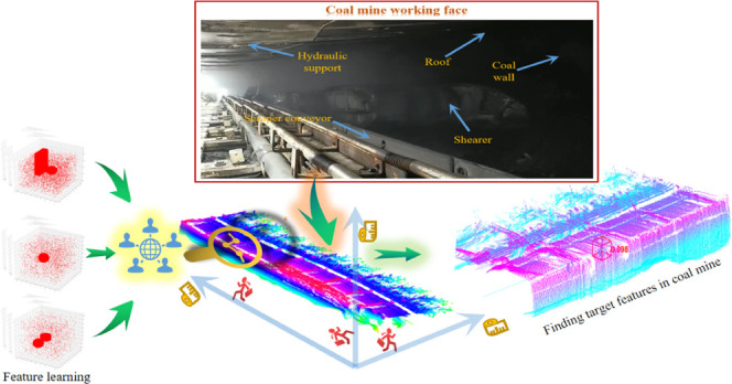
We drive the inspection robot with battery power and carry the LiDAR to realize rapid movement so as to collect the point cloud of the whole coal mine working face. Most importantly, we propose MS-DGCNN to find the ball in the large-scale point cloud data of the coal mining environment (Figure 1).
Figure 1.
MS-DGCNN is trained in the point cloud data set we have made (bottom) and the trained MS-DGCNN identifies the ball in the point cloud of the coal mine working face (top).
2.1. Edge Convolution Operation on Graph Structure
In this study, point cloud data can be represented as graph structure data, each point in the point cloud can be represented by vertices in the graph structure, and the relationship between two points in the point cloud can be represented by edges connecting vertices. The degree matrix D on the graph structure only has values on the diagonal, and the rest are 0. The internal value of adjacency matrix A is 1 only between two nodes with edge links, and 0 in other places, which is used to describe the topology of the graph.38 Laplace matrix L is D–A. It can be expressed as eq 1.
 |
1 |
where d is the degree of the node and a is the edge relationship between the two nodes. Since the L matrix is a positive semidefinite symmetric matrix, we can perform spectral decomposition of the L matrix to obtain eq 2.
 |
2 |
where C is a matrix in which the column vector is a unit eigenvector, C is an n eigenvector of L, C = (c⃗1, c⃗2, ..., c⃗n), and δn represents the eigenvalue corresponding to the nth eigenvector.
We change the eigenfunction of the Laplacian operator into the eigenvector of the Laplacian matrix in the graph structure so as to obtain the Fourier transform on the graph structure, such as eq 3.39,40
| 3 |
where f is the N-dimensional vector on the graph structure, f(δ) corresponds to the nodes on the graph one by one, cl*(i) represents the ith component of the lth eigenvector, and the Fourier transform of f on the graph structure data is essentially the inner product operation of the eigenvector corresponding to δl and cl. The above inner product operation is defined in the complex space, so cl(i) is adopted, that is, the conjugate of the eigenvector cl. We use matrix multiplication to extend the Fourier transform on the graph structure to the matrix form, such as eq 4.
 |
4 |
Similarly, we can obtain the matrix form of the inverse Fourier transform on the graph structure. Based on the above data, we first define the theorem of convolution, as shown in eq 5.41,42
| 5 |
For functions f and p, their convolution is the inverse transformation of their Fourier transform product. Second, we extend convolution to the graph structure and use edge links to represent the relationship between two nodes. Finally, we bring the Fourier transform of the graph defined in eq 3 into eq 5 to obtain the definition of convolution operation on the graph structure, as shown in eq 6.
 |
6 |
where ⊙ is the operation symbol of Hadamard product, which means element by element multiplication for two-point cloud data with the same dimension. The internal propagation rule of DGCNN is expressed as eq 7.
| 7 |
where H is the eigenvector of nodes in the graph structure, where H(0) = X. X ∈ RN*D, X is the feature matrix of N*D (N is the number of nodes and D is the dimension of input feature); l is the number of layers of the model; σ is the activation function; Â = A + I, where A is the adjacency matrix and I is the identity matrix; D̂ is the diagonal matrix of Â; and W(l) is the perceptron model. The feature of the center point vi in the l + 1 layer can be expressed as eq 8.
| 8 |
where j is the neighbor node index of the central point vi, Ni is all neighbors of the central point vi, Cij is the normalized constant of the edge, and hvi(l) is the feature of the node vi in the L layer. Based on the above theory, edge convolution extracts the edge features between the center point and several neighbor points, and then aggregates the edge feature, which considers the local feature of point cloud.
2.2. Method of Multiscale Edge Convolution
The point cloud in the edge convolution is represented in the form of a directed graph. The node is each point in the point cloud, and the set of nodes is represented by eq 9.
| 9 |
where n represents the number of point clouds and F represents the dimension of point clouds. The feature of the edge can be expressed as eq 10.
| 10 |
where hΘ: RF × RF → RF′, Θ is a learnable parameter, Θ = (θ1, ..., θi, ϕ1, ..., ϕi); xi represents the currently selected center point, i = 1, 2, ..., n; and xj represents the adjacent point near the center point, where j depends on the value of K in edge convolution. Therefore, different K values affect the local feature of point cloud extracted by DGCNN.
The aggregation operation of the center point can finally be expressed as eq 11.43
| 11 |
where m represents the number of feature channels, θ and ϕ are the learning parameters of Θ; and ε represents the edges in the graph structure.
In addition, point cloud data is a low-resolution sampling of the three-dimensional physical world, which has the characteristic of uneven density, as shown in Figure 2.
Figure 2.
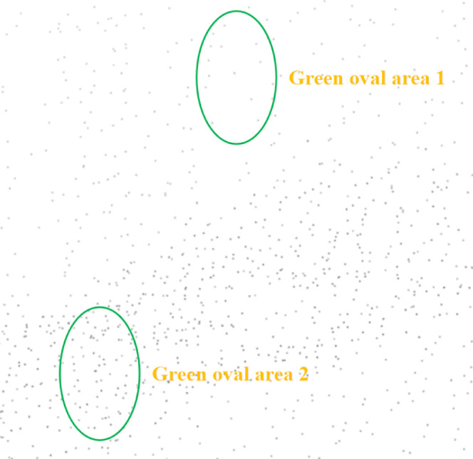
Local enlargement of point cloud in coal mine working face.
In Figure 2, the area size of the green ellipse is the same, but the number of points in the point cloud is different, which will lead to some missing or redundant local feature areas in the point cloud extracted by the single-scale edge convolution in DGCNN. Therefore, based on the previously established DGCNN, we have proposed multiscale edge convolution to extract the local feature of point cloud. This can not only solve the problems of single-scale edge convolution, but also multiscale edge convolution uses different scales to construct dynamic local neighborhoods and splice the feature extracted in different scale regions so that the local feature of point cloud can be learned at more levels.
Through the preliminary research of the research group where the author works, it is known that when K = 20, the performance of DGCNN is the best. In this study, K = 10, 20, and 30 are used to extract the neighborhood features of different scales for each central point, and the local feature of different scales are spliced. We analyze the performance of DGCNN under multiscale and different single-scale edge convolution in Section 3.1.
2.3. Processing Method of Point Cloud Disorder
The point cloud has the characteristics of disorder, that is, the information expressed by the point cloud will be not changed, no matter how the position of each point in the point cloud is permuted. This requires a symmetric function to ensure the disorder of point cloud. The symmetric function can be expressed by eq 12.
| 12 |
where x1, x2, ..., xn represents each point in the point cloud, respectively, and π represents the permutation function.
We can know that for a point cloud with n points, there are n factorial permutations. DGCNN uses the symmetric function max-pooling to meet the permutation invariance of the point cloud after edge convolution and uses max-pooling to obtain the global feature of the point cloud, as shown in eq 13.
| 13 |
where G represents the global feature of the point cloud, [E(x1), E(x2), ..., E(xn)] represents the output of the point cloud after multilayer edge convolution, and max represents the max-pooling operation.
However, using the max-pooling operation to deal with the disorder of point cloud will lead to the loss of point cloud information. Because average-pooling is an operation considering the feature of all points in the point cloud, we have added average-pooling as a symmetric function to extract the global feature in the point cloud on the basis of the max-pooling, which can not only ensure the disorder of the point cloud but also effectively solve the problem of global information loss caused by the existing max-pooling in DGCNN. As shown in eq 14.
| 14 |
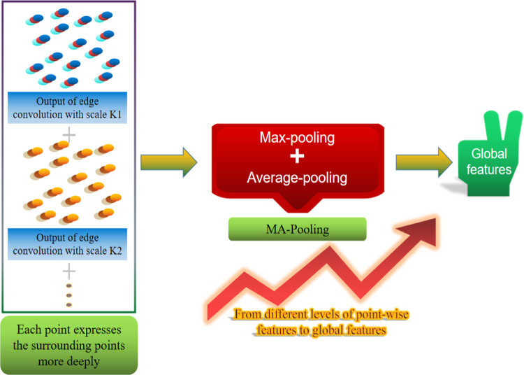
where mean represents the average-pooling operation. The MA-pooling operation of the point cloud after edge convolution is shown in Figure 3.
Figure 3.
MA-pooling of point clouds after edge convolution at different scales.
As shown in Figure 3, after multiscale edge convolution, the local features of the point cloud are fully learned. We splice the feature of point cloud after edge convolution at different scales and then use MA-pooling to better extract the global feature of point cloud. We compare the effects of DGCNN on MA-pooling and max-pooling in Section 3.2.
2.4. Data Set Description
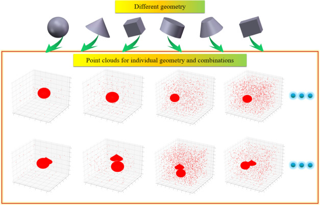
To make different deep neural network models fully learn the feature of the ball, we first generate a variety of geometries including the ball. Second, we set the positions of all geometry to be random within a certain range, including complete balls and incomplete balls appearing. And we generate point clouds from a variety of individual geometries and combinations in different cases. Finally, we add different degrees of noise to each point cloud file in the data set so that the deep neural network can deeply learn the feature of each geometry, as shown in Figure 4 (because there are too many kinds of geometry, we select the point cloud of balls, combination of ball and cuboid, combination of ball and cone, and combination of ball and cube for display).
Figure 4.
Point cloud data set with different degrees of noise added.
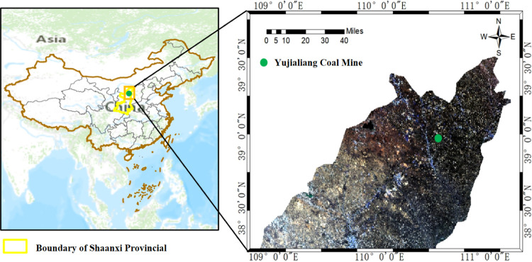
To verify the correctness of our proposed method, we have collected the point cloud of coal mine working face on the spot. Shendong Coal Group of China National Energy Group has several production mines, among which Yujialiang coal mine has a mine field area of 56.33 km2, a mine geological storage of 504 million tons, and a recoverable storage of 355 million tons. We have cooperated with Shendong Coal Group to arrange the underground inspection robot purchased and developed by us in Yujialiang coal mine. The location of Yujialiang coal mine is shown in Figure 5.
Figure 5.
Location of Yujialiang coal mine.
Due to the harsh underground working environment, our research team have installed a protective cover outside the LiDAR of the underground inspection robot to prevent damage and interference from external objects. The underground inspection robot is equipped with LiDAR and runs on the flexible track arranged on one side of the cable trough of the scraper conveyor, and the springs with certain bearing capacity are used between the tracks so as to scan and collect the large-scale point cloud of the whole coal mine working face, as shown in Figure 6. We have used the trained different deep neural networks to identify the ball point cloud in the point cloud of the coal mine working face by sliding the window. If there is a ball point cloud in the current window, the error of the ball center position between the found ball and the real ball will be calculated.
Figure 6.
Equipment for obtaining point cloud of the coal mine working face.
The collected point cloud of the whole coal mine working face is shown in Figure 7. Because the number of point clouds in the whole coal mine working face reaches tens of millions, the range of point clouds in the X direction is 0–350 m. To intuitively and clearly observe the effect of different deep neural networks, we have visualized the local segment of the point cloud of the coal mine working face where the ball is located.
Figure 7.
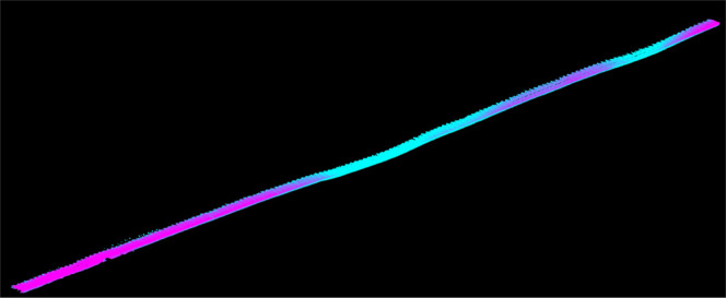
Point cloud of the whole coal mine working face.
2.5. Experimental Details
The central processing unit of the experimental platform of this study is Intel Core(R) CPU I7-9700@3.00GHz×8. The graphics processing unit is NVIDIA GTX 2080 Super. The momentum factor is set to 0.9, and the weight attenuation coefficient is set to 10–4. The K of edge convolution is set to 10, 15, 20, 25, and 30, respectively, to observe the performance of DGCNN under single-scale edge convolution and multiscale edge convolution. To prevent overfitting, dropout is used in the full connection layer. We have selected the variant of ReLU (Leaky ReLU) as the activation function. Leaky ReLU changes the method of complete inhibition of nonpositive part in ReLU and gives it a smaller slope value. Adaptive motion estimation (Adam) is used in the training process of deep neural network.44−47
We use accuracy and loss to evaluate the performance of different networks. Accuracy indicates the proportion of all samples correctly predicted in all test samples. Accuracy can be expressed as eq 15.48
| 15 |
where TP (true positive) represents the number of samples whose actual category and prediction category are positive category. FP (false positive) represents the number of samples whose actual category belongs to negative category but is predicted to be positive category. FN (false negative) represents the number of samples whose actual category belongs to positive category but is predicted to be negative category. TN (true negative) represents the number of samples whose actual category and prediction category are negative category.
Cross-entropy loss function is a way to measure the predicted value and actual value of neural network. The loss of neural network is the calculation result of cross-entropy loss function, and its calculation formula can be expressed as eq 16.49,50
| 16 |
where N is the number of samples, K is the category of samples, p(x) is the probability distribution of the expected output for sample x, and q(x) is the probability distribution of the predicted output for sample x. Therefore, it can be seen that the larger the accuracy and the smaller loss, the better the performance of the neural network.
We have used the confusion matrix to analyze the extraction effect of different networks on each geometric feature and verified the results of accuracy and loss. The confusion matrix CM can be expressed as eq 17.51,52
 |
17 |
where n represents the number of samples and m represents the category of samples. The element in row i and column j represents the number of class i identified as class j by classifier C in the sample. Under the ideal condition, the accuracy of the neural network is 100%, then the nondiagonal elements of the confusion matrix are 0, and only the diagonal elements are non-0.
In this study, six kinds of geometric point clouds were generated, including the ball, and we represent each individual geometric point cloud with a one-digit code (if there is a geometric feature, its corresponding number is 1, and if there is no geometric feature, its corresponding number is 0) and then traverse to generate all geometric feature digital codes. The main MATLAB R2019a code is shown in Table S1.
There are 64 features in the point cloud data set (including 00000, which indicates that there are no geometric feature and only noise points). If the results are represented by numbers in each square in the confusion matrix, it will be too confusing in the sense. To make the confusion matrix more clear and intuitive, we have used different colors to represent each square in the confusion matrix. The closer the color is to dark red, the higher the accuracy is, and the closer the color is to dark blue, the lower the accuracy is. In addition, we have added the main core MATLAB R2019a code that randomly generated different numbers of noise points within a certain coordinate range, as shown in Table S2.
Only after the deep neural network model learns the feature of geometric point cloud more deeply and fully, it can find geometric point cloud more accurately in the point cloud of coal mine working face. We have replaced the test set with the coal mine working face point cloud, further analyzed the robustness of multiscale edge convolution, MA-pooling, and MS-DGCNN, and have provided a new method for geometric feature perception in the coal mine working face point cloud.
The real ball center position in the coal mine working face has been obtained in MATLAB R2019a. We use the error of the ball center position to evaluate the effect of the deep neural network model on finding the ball point cloud. The error of the ball center position (EBCP) expression is shown in eq 18.
| 18 |
where x1, y1, and z1 represent the real ball center position and x2, y2, and z2 represent the ball center position found by the deep neural network. We finally select the minimum EBCP display obtained by each network model.
3. Results
3.1. Comparison of Results of Single-Scale and Multiscale Edge Convolutions
The point cloud has an unstructured characteristic. The original DGCNN uses single-scale edge convolution (single K value) to extract the local feature of the point cloud (according to our previous research results, it is known that the performance of DGCNN is better when K = 20). We have analyzed the loss and accuracy of DGCNN under multiscale edge convolution and single-scale edge convolution (K = 10, K = 15, K = 20, K = 25, K = 30), as shown in Figures 8 and 9, respectively.
Figure 8.
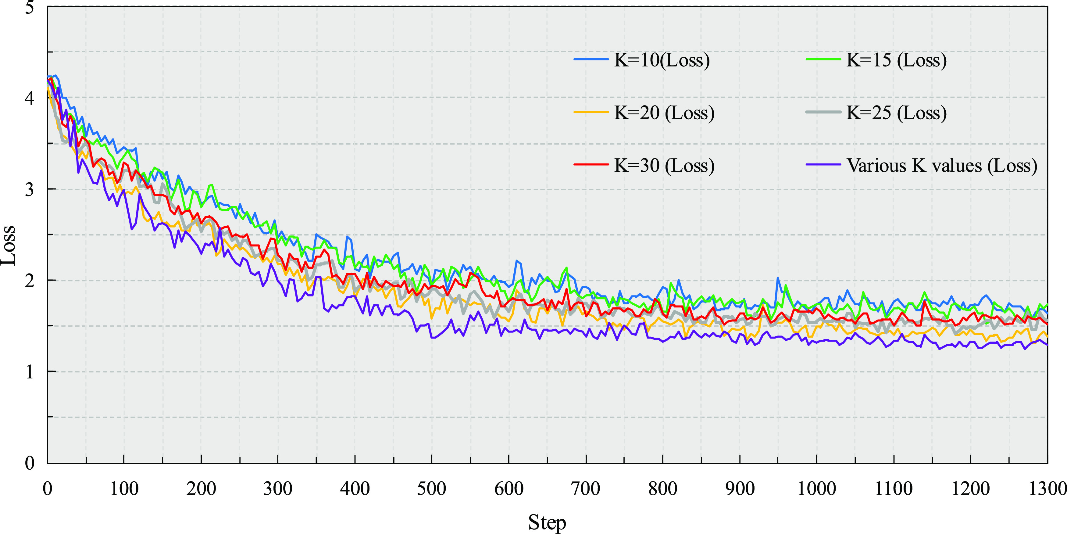
Loss of DGCNN under multiscale and single-scale edge convolutions.
Figure 9.
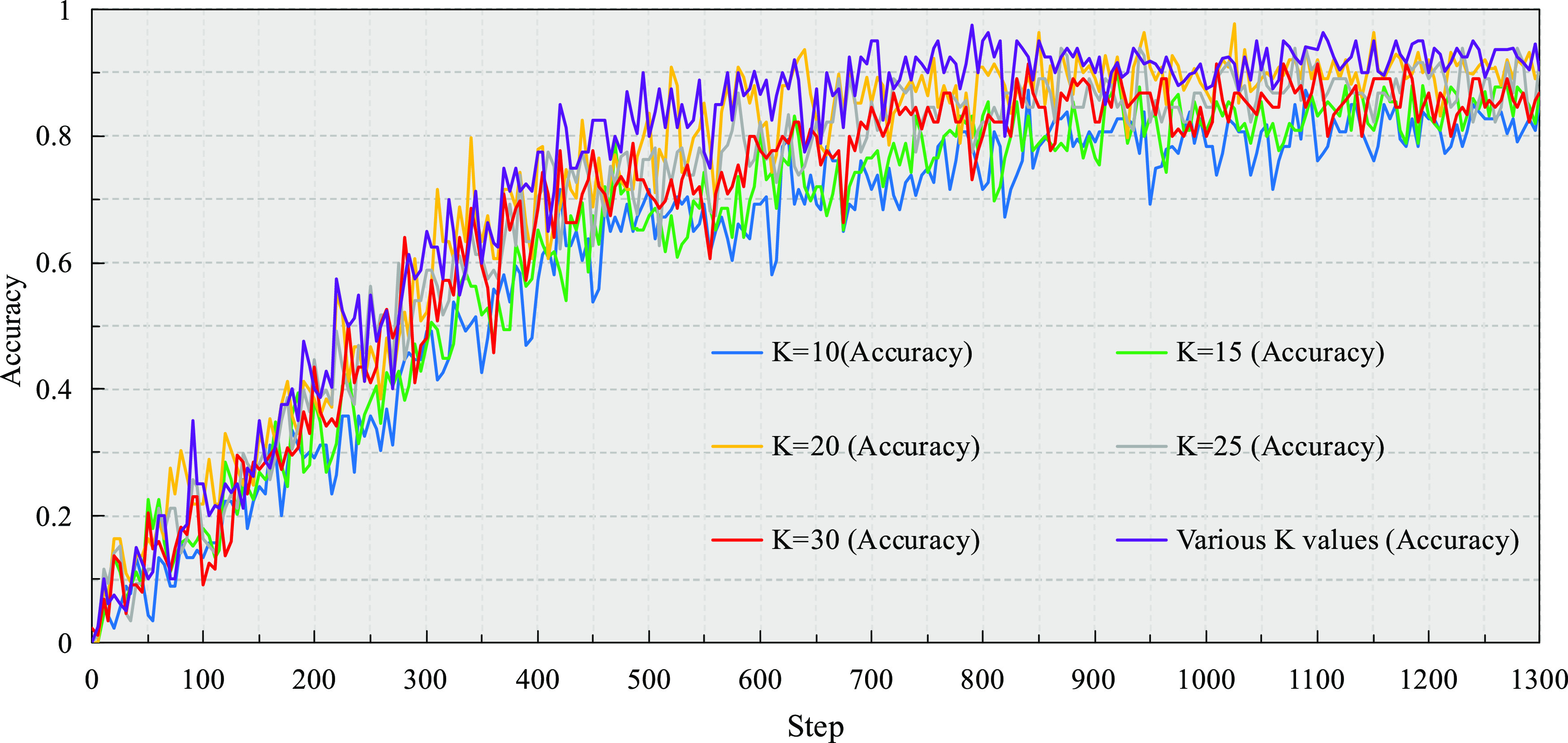
Accuracy of DGCNN under multiscale and single-scale edge convolutions.
We can see that when the accuracy and loss tend to be stable, the accuracy obtained by DGCNN under multiscale edge convolution is greater than that obtained by DGCNN under different single-scale edge convolutions. At the same time, the loss obtained by DGCNN under multiscale edge convolution is less than that obtained by DGCNN under different single-scale edge convolutions. Therefore, DGCNN under multiscale edge convolution achieves the best effect.
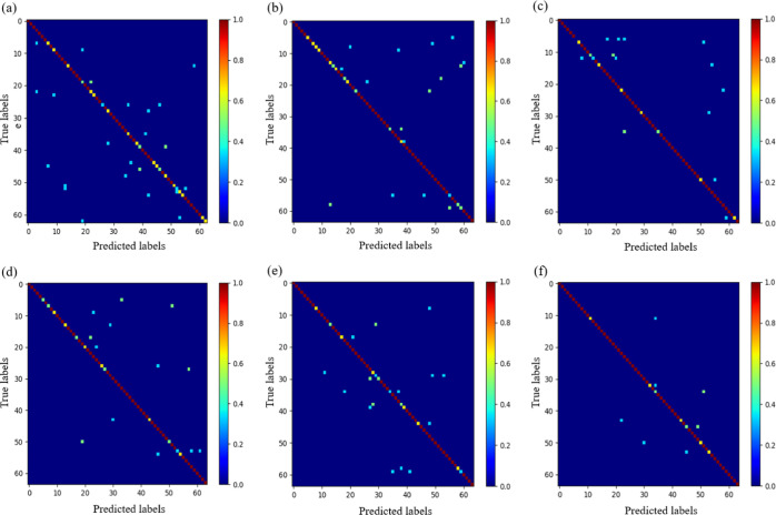
We have obtained the confusion matrix of DGCNN under multiscale edge convolution and different single-scale edge convolutions, as shown in Figure 10.
Figure 10.
Confusion matrix of DGCNN under multiscale and single-scale edge convolutions: (a) K = 10, (b) K = 15, (c) K = 20, (d) K = 25, (e) K = 30, and (f) various K values.
In Figure 10, the closer the color in each square is to dark red, the higher the accuracy is, and the closer the color in each square is to dark blue, the lower the accuracy is. We can see that DGCNN under multiscale edge convolution has the best effect in the case of a single geometric feature, as well as in the case of multiple geometric features at the same time. It fully shows that DGCNN of multiscale edge convolution can learn the geometric feature of point cloud more deeply.
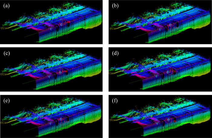
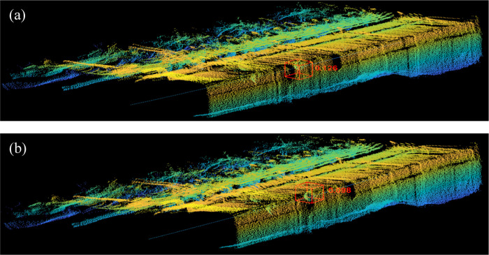
Finally, we have obtained the effect of DGCNN identifying the ball in the point cloud of coal mine working face under multiscale edge convolution and different single-scale edge convolutions, as shown in Figure 11.
Figure 11.
Effects of different single-scale edge convolutions and multiscale edge convolution: (a) K = 10, (b) K = 15, (c) K = 20, (d) K = 25, (e) K = 30, and (f) various K values.
As can be seen from Figure 11, DGCNN in different cases has highlighted the point cloud of the ball they found with a red box, and the number on the side of the box is the EBCP between the ball found by the deep neural network and the real ball. When K = 10, K = 15, K = 20, K = 20, K = 30 and various K values, EBCP is 0.268, 0.260, 0.144, 0.179, 0.208, and 0.126 respectively. DGCNN under multiscale edge convolution shows the best performance, which is consistent with the results obtained by comparing the performance of DGCNN under accuracy, loss, and confusion matrix.
3.2. Comparison of Results between MA-Pooling and Max-Pooling
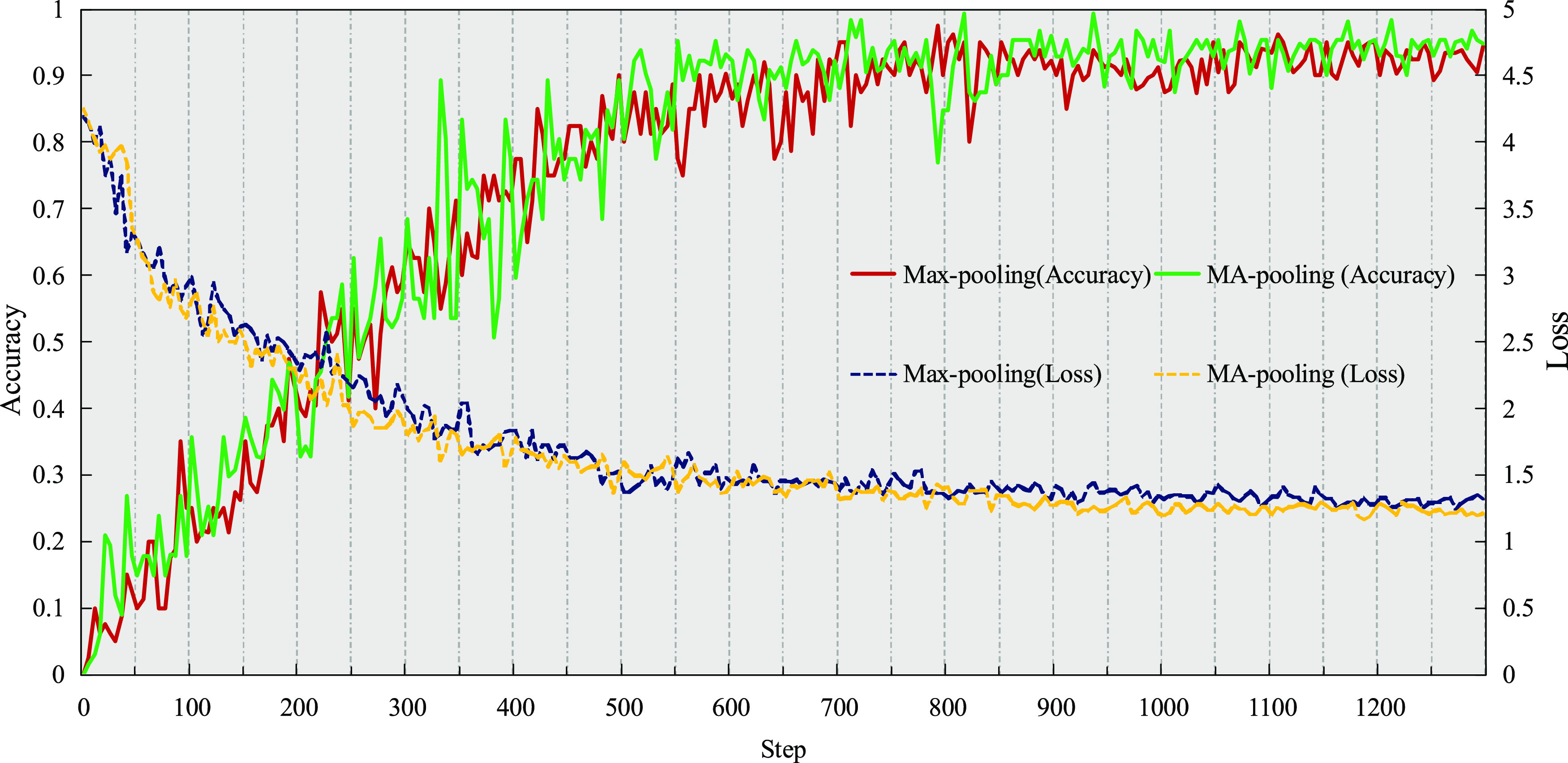
Point cloud has the characteristics of not only nonuniformity but also disorder. The deep neural networks that directly process point clouds use max-pooling as a symmetric function to meet the displacement invariance of point clouds and use max-pooling to obtain the global feature of point clouds. We have proposed to upgrade max-pooling to MA-pooling and the accuracy and loss of MS-DGCNN under MA-pooling and max-pooling, as shown in Figure 12.
Figure 12.
Accuracy and loss of MS-DGCNN under MA-pooling and max-pooling.
As can be seen from Figure 12, MS-DGCNN under MA-pooling is higher than MS-DGCNN under max-pooling in terms of accuracy, and MS-DGCNN under MA-pooling is lower than MS-DGCNN under max-pooling in terms of loss. MS-DGCNN under MA-pooling has achieved the best results in both accuracy and loss.
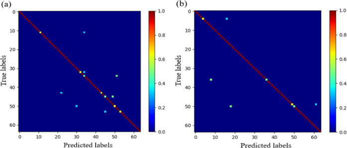
The confusion matrix of MS-DGCNN under max-pooling and MA-pooling is shown in Figure 13.
Figure 13.
Confusion matrix of MS-DGCNN under max-pooling and MA-pooling: (a) max-pooling and (b) MA-pooling.
From Figure 13, we can see that MS-DGCNN under MA-pooling has the best point cloud classification effect for a single feature, and the point cloud classification effect for multiple features is also the best. It is remarkable that when some geometric features appear at the same time and the features are not obvious, the effect of MS-DGCNN under MA-pooling is still the best, which fully shows that MS-DGCNN under MA-pooling shows better performance than MS-DGCNN under max-pooling.
The effect of MS-DGCNN under max-pooling and MS-DGCNN under MA-pooling on identifying the ball in the point cloud of coal mine working face is shown in Figure 14.
Figure 14.
Effects of (a) max-pooling and (b) MA-pooling.
It can be seen that the EBCP of MS-DGCNN under MA-pooling to identify the ball in the point cloud of coal mine working face is lower than that of MS-DGCNN under max-pooling, which shows that MS-DGCNN under MA-pooling can better extract the geometric feature of the ball point cloud. In addition, it also shows that MS-DGCNN using MA-pooling has strong generalization, and its ability to identify the ball in the point cloud of coal mine working face is still better than MS-DGCNN using max-pooling.
4. Discussion
The main reasons why DGCNN under multiscale edge convolution is better than that under single-scale (K = 10, K = 15, K = 20, K = 25, K = 30) edge convolution are as follows: point cloud is a kind of data obtained by randomly collecting discrete points on a three-dimensional physical surface. The irregular distribution of point cloud data makes the density of points in different regions different. When DGCNN selects a fixed single K value, some of the local feature regions of the point cloud extracted by edge convolution will be missing and some will be redundant. Multiple K values can not only overcome the above shortcomings to a certain extent, but more importantly, the multiple K values proposed in this study can obtain feature representation with higher dimensions and richer local details, and the local feature of point cloud can be extracted more fully and at more levels by edge convolution so that DGCNN under multiscale edge convolution can obtain a more powerful feature expression ability.
The main reason why MS-DGCNN under MA-pooling achieves better results than MS-DGCNN under max-pooling is that only the max-pooling layer is used to deal with the disorder of point cloud and extract global feature. However, such an operation will lose the information of all points except the point with the maximum eigenvalue in each dimension. MA-pooling combines max-pooling and average-pooling as symmetric functions. With the advantage that average-pooling retains the global feature, average-pooling is obtained by considering the feature of each point in the point cloud. This improvement makes up for the information loss caused by the use of max-pooling alone. Therefore, MA-pooling can get more abundant global feature information of point cloud, which makes MS-DGCNN have stronger robustness and classification performance.
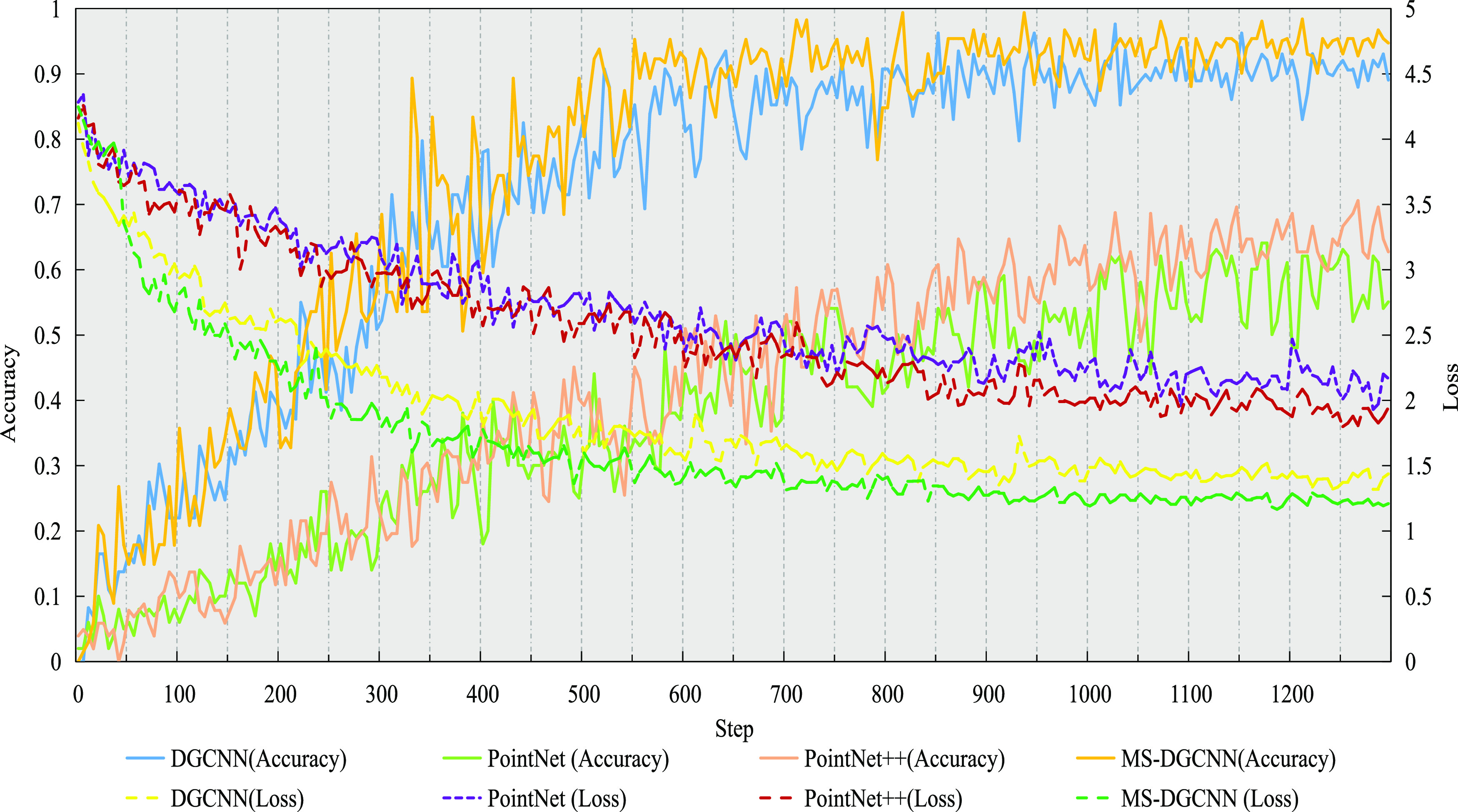
We have compared MS-DGCNN with MA-pooling and DGCNN (K value is 20, and max-pooling is used to extract global feature). Furthermore, we have added another deep neural network (PointNet), which directly processes point clouds and PointNet++ (an improved version of PointNet), to the comparative experiment. The accuracy and loss results of MS-DGCNN, DGCNN, PointNet, and PointNet++ are shown in Figure 15.
Figure 15.
Accuracy and loss of MS-DGCNN, DGCNN, PointNet, and PointNet++.
As can be seen from Figure 15, in terms of loss, the performance of different deep neural networks from good to bad is ranked as MS-DGCNN, DGCNN, PointNet, and PointNet++. In terms of accuracy, the performance of different deep neural networks from good to bad is also ranked as MS-DGCNN, DGCNN, PointNet, and PointNet++.
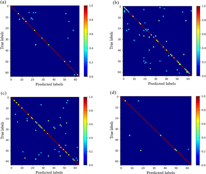
We analyze the confusion matrix of MS-DGCNN, DGCNN, PointNet, and PointNet++, as shown in Figure 16.
Figure 16.
Confusion matrix of DGCNN, PointNet, PointNet++, and MS-DGCNN: (a) DGCNN, (b) PointNet, (c) PointNet++, and (d) MS-DGCNN.
As can be seen from Figure 16, MS-DGCNN not only shows the best performance when there are only individual geometric features in the point cloud. When there are many geometric features in the point cloud, MS-DGCNN also shows the best performance. The results are the same as that obtained using accuracy and loss as evaluation indexes.
This is because PointNet can only learn the global feature of the point cloud without considering the local feature of the point cloud. PointNet++ uses multiple PointNets to consider the local structure of point cloud, but PointNet++ does not break away from the bondage of PointNet in essence. Although DGCNN uses edge convolution to extract the local feature of point cloud, it uses single-scale edge convolution to result in the number of points in each local region. DGCNN, PointNet, and PointNet++ use max-pooling to extract the global feature of point cloud, resulting in the loss of point cloud information to a certain extent. On the one hand, MS-DGCNN uses multiscale edge convolution to splice and combine the local feature of point cloud extracted at each scale to obtain local features with higher dimensions and richer local details. On the other hand, MA-pooling makes up for the loss of global information caused by max-pooling alone and can better extract the global feature of point cloud.
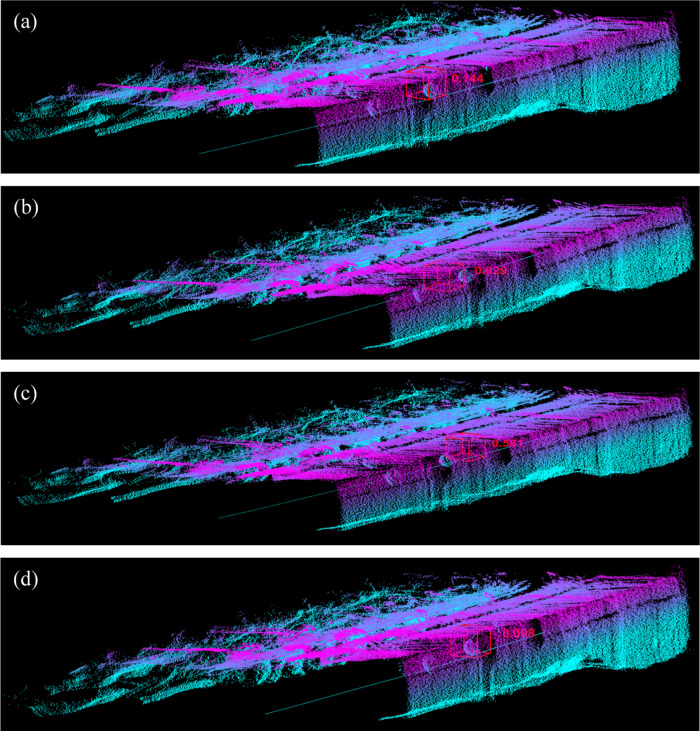
We have used PointNet, PointNet++, DGCNN, and MS-DGCNN proposed in this research to identify the ball in the actually collected point cloud of coal mine working face. The results are shown in Figure 17.
Figure 17.
DGCNN, PointNet, PointNet, and MS-DGCNN identify the ball point cloud: (a) DGCNN, (b) PointNet, (c) PointNet++, and (d) MS-DGCNN.
As can be seen from Figure 17, the EBCPs corresponding to DGCNN, PointNet, PointNet++, and MS-DGCNN are 0.144, 0.629, 0.581, and 0.098 respectively, and MS-DGCNN obtains the minimum EBCP. This is because, on the one hand, MS-DGCNN solves the problem that some local features of point cloud extracted by edge convolution under a single K value will be missing and some will be redundant. On the other hand, edge convolution can extract local feature of point cloud at a deeper and more level under a variety of K values. In addition, MS-DGCNN solves the problem of information loss when DGCNN, PointNet, and PointNet++ extract the global feature of point cloud in the coal mine working face. Therefore, the MS-DGCNN we have proposed and constructed can better extract the global and local features in point cloud data and achieve better performance. More importantly, this research reflects the practical application value of the MS-DGCNN we have constructed. The MS-DGCNN we proposed can more accurately identify the point cloud of the ball in the point cloud of the coal mine working face, which provides a solid foundation for the geometric feature identification in the environmental perception of the coal mine working face.
Finally, it is remarkable that the inspection robot installed with LiDAR has vibration and shaking, as well as collecting the point cloud of coal mine working face, coupled with the influence of adverse factors, such as coal dust and water mist on coal mine working face and so on. The geometry point cloud training set in this study is generated for the ball point cloud of coal mine working face. At the same time, our proposed method is also aiming at the point cloud of coal mine working face. Therefore, although the method we proposed in this study can identify the target geometry (ball) in the point cloud of coal mine working face, we need to consider how this method can identify the target geometry in other point cloud scenes.
5. Conclusions
Based on our previous work, MS-DGCNN (integrating multiscale edge convolution and MA-pooling) is proposed for the first time to identify the geometric feature of point cloud in coal mine working face. The main conclusions of this study are as follows: (1) We use multiscale edge convolution, which not only overcomes the defect that the local feature of point cloud extracted by single-scale edge convolution will be missing or be redundant but also extracts the local feature representation of point cloud deeper and richer from multiple angles so that MS-DGCNN can obtain more powerful feature expression ability. (2) Average-pooling is a pooling operation that takes into account each feature in the point cloud. We proposed a method combining max-pooling and average-pooling (MA-pooling) to extract the global feature of point cloud, and we took MA-pooling as the symmetry function of MS-DGCNN. This achievement not only meets the displacement invariance of point cloud but also makes up for the loss of certain global feature information of point cloud caused by using max-pooling alone. (3) We have used MS-DGCNN, DGCNN, PointNet, and PointNet++ to extract the feature of various geometric point clouds and identify the target geometry in the large-scale point cloud of coal mine working face (in this study, we take the ball as an example). MS-DGCNN has obtained the best effect, which fully explains the powerful feature expression ability and generalization performance of MS-DGCNN. The lack of accurate environmental perception ability of coal mine working face has always been one of the important factors hindering the development of transparency of working face. This study provides a solid foundation for geometric feature identification in the environmental perception of coal mine working face and makes a beneficial exploration on promoting the development of transparency of working face. Most importantly, this study innovates the research method of environmental perception of coal mine working face.
Acknowledgments
This study was supported by the National Key R&D Program of China (grant no. 2017YFC0804310), the Key R&D Projects of Shaanxi Province (grant nos. 2019ZDLGY03-09-02, 2020ZDLGY04-05, and 2020ZDLGY04-06) and the General Special Scientific Research Plan of Shaanxi Provincial Department of Education (grant no. 20JK0754). The authors thank the reviewers and editors for their constructive comments and suggestions on improving this manuscript.
Supporting Information Available
The Supporting Information is available free of charge at https://pubs.acs.org/doi/10.1021/acsomega.1c05473.
Main code for generating all geometric features and the main code for adding noise points to geometry point cloud (PDF)
The authors declare no competing financial interest.
Supplementary Material
References
- Santamarina J. C.; Torres-Cruz L. A.; Bachus R. C. Why coal ash and tailings dam disasters occur. Science 2019, 364, 526–528. 10.1126/science.aax1927. [DOI] [PubMed] [Google Scholar]
- Li X.; Chen X.; Zhang F.; Zhang M.; Zhang Q.; Jia S. Energy Calculation and Simulation of Methane Adsorbed by Coal with Different Metamorphic Grades. ACS Omega 2020, 5, 14976–14989. 10.1021/acsomega.0c00462. [DOI] [PMC free article] [PubMed] [Google Scholar]
- Li L.; Liu D.; Cai L.; Wang Y.; Jia Q. Coal Structure and Its Implications for Coalbed Methane Exploitation: A Review. Energy Fuels 2021, 35, 86–110. 10.1021/acs.energyfuels.0c03309. [DOI] [Google Scholar]
- Wang G.; Xu Y.; Ren H. Intelligent and ecological coal mining as well as clean utilization technology in China: Review and prospects. Int. J. Min. Sci. Technol. 2019, 29, 161–169. 10.1016/j.ijmst.2018.06.005. [DOI] [Google Scholar]
- Xiao D.; Li H.; Sun X. Coal Classification Method Based on Improved Local Receptive Field-Based Extreme Learning Machine Algorithm and Visible–Infrared Spectroscopy. ACS Omega 2020, 5, 25772–25783. 10.1021/acsomega.0c03069. [DOI] [PMC free article] [PubMed] [Google Scholar]
- Sonter L. J.; Dade M. C.; Watson J. E.; Valenta R. K. Renewable energy production will exacerbate mining threats to biodiversity. Nat. Commun. 2020, 11, 4174 10.1038/s41467-020-17928-5. [DOI] [PMC free article] [PubMed] [Google Scholar]
- Wang J.; Huang Z. The recent technological development of intelligent mining in China. Engineering 2017, 3, 439–444. 10.1016/J.ENG.2017.04.003. [DOI] [Google Scholar]
- Liu H.; Wang F.; Ren T. Research on the characteristic of the coal–oxygen reaction in a lean-oxygen environment caused by methane. Energy Fuels 2019, 33, 9215–9223. 10.1021/acs.energyfuels.9b01753. [DOI] [Google Scholar]
- Liu J.; Yang T.; Wang L.; Chen X. Research progress in coal and gas co-mining modes in China. Energy Sci. Eng. 2020, 8, 3365–3376. 10.1002/ese3.739. [DOI] [Google Scholar]
- Jo B. W.; Khan R. M. A.; Javaid O. Arduino-based intelligent gases monitoring and information sharing Internet-of-Things system for underground coal mines. J. Ambient Intell. Smart Environ. 2019, 11, 183–194. 10.3233/AIS-190518. [DOI] [Google Scholar]
- Zhai G.; Zhang W.; Hu W.; Ji Z. Coal mine rescue robots based on binocular vision: A review of the state of the art. IEEE Access 2020, 8, 130561 10.1109/ACCESS.2020.3009387. [DOI] [Google Scholar]
- Igathinathane C.; Ulusoy U. Machine vision methods based particle size distribution of ball-and gyro-milled lignite and hard coal. Powder Technol. 2016, 297, 71–80. 10.1016/j.powtec.2016.03.032. [DOI] [Google Scholar]
- Xu J.; Wang E.; Zhou R. Real-time measuring and warning of surrounding rock dynamic deformation and failure in deep roadway based on machine vision method. Measurement 2020, 149, 107028 10.1016/j.measurement.2019.107028. [DOI] [Google Scholar]
- Qiao T.; Liu W.; Pang Y.; Yan G. Research on visible light and infrared vision real-time detection system for conveyor belt longitudinal tear. IET Sci., Meas. Technol. 2016, 10, 577–584. 10.1049/iet-smt.2015.0297. [DOI] [Google Scholar]
- Cui Y.; Liu S.; Yao J.; Gu C. Integrated Positioning System of Unmanned Automatic Vehicle in Coal Mines. IEEE Trans. Instrum. Meas. 2021, 70, 1–13. 10.1109/TIM.2021.3083903.33776080 [DOI] [Google Scholar]
- Cao B.; Wang S.; Ge S.; Ma X.; Liu W. A novel mobile target localization approach for complicate underground environment in mixed LOS/NLOS scenarios. IEEE Access 2020, 8, 96347–96362. 10.1109/ACCESS.2020.2995641. [DOI] [Google Scholar]
- Li M.; Zhu H.; You S.; Tang C. UWB-Based Localization System Aided With Inertial Sensor for Underground Coal Mine Applications. IEEE Sens. J. 2020, 20, 6652–6669. 10.1109/JSEN.2020.2976097. [DOI] [Google Scholar]
- Zheng X.; Wang B.; Guo J.; Zhang D.; Zhao J. Factors influencing dielectric properties of coal of different ranks. Fuel 2019, 258, 116181 10.1016/j.fuel.2019.116181. [DOI] [Google Scholar]
- a Wu G.; Fang X.; Zhang L.; Liang M.; Lv J.; Quan Z. Positioning Accuracy of the Shearer Based on a Strapdown Inertial Navigation System in Underground Coal Mining. Appl. Sci. 2020, 10, 2176 10.3390/app10062176. [DOI] [Google Scholar]; b Miao Q.; Liu C.; Zhang N.; Lu K.; Gu H.; Jiao J.; Zhang J.; Wang Z.; Zhou X. Toward Self-Powered Inertial Sensors Enabled by Triboelectric Effect. ACS Appl. Electron. Mater. 2020, 2, 3072–3087. 10.1021/acsaelm.0c00644. [DOI] [Google Scholar]
- Cui Y.; Liu J.; Yao J.; Gu C. Integrated Positioning System of Unmanned Automatic Vehicle in Coal Mines. IEEE Trans. Instrum. Meas. 2021, 70, 1–13. 10.1109/TIM.2021.3083903.33776080 [DOI] [Google Scholar]
- Mellors R.; Yang X.; White J. A.; Ramirez A.; Wagoner J.; Camp D. W. Advanced geophysical underground coal gasification monitoring. Mitigation Adapt. Strategies Global Change 2016, 21, 487–500. 10.1007/s11027-014-9584-1. [DOI] [Google Scholar]
- Yim G.; Ji S.; Cheong Y.; Neculita C. M.; Song H. The influences of the amount of organic substrate on the performance of pilot-scale passive bioreactors for acid mine drainage treatment. Environ. Earth Sci. 2015, 73, 4717–4727. 10.1007/s12665-014-3757-9. [DOI] [Google Scholar]
- Liang M.; Fang X.; Li S.; Wu G.; Ma M.; Zhang Y. A fiber Bragg grating tilt sensor for posture monitoring of hydraulic supports in coal mine working face. Measurement 2019, 138, 305–313. 10.1016/j.measurement.2019.02.060. [DOI] [Google Scholar]
- Guo P.; Su Y.; Pang D.; Wang Y.; Guo Z. Numerical study on heat transfer between airflow and surrounding rock with two major ventilation models in deep coal mine. Arabian J. Geosci. 2020, 13, 756 10.1007/s12517-020-05725-9. [DOI] [Google Scholar]
- Du T.; Nie W.; Chen D.; Xiu Z.; Yang B.; Liu Q.; Guo L. CFD modeling of coal dust migration in an 8.8-meter-high fully mechanized mining face. Energy 2020, 212, 118616 10.1016/j.energy.2020.118616. [DOI] [Google Scholar]
- Cheng M.; Fu X.; Kang J.; Tian Z.; Shen Y. Experimental Study on the Change of the Pore-Fracture Structure in Mining-Disturbed Coal-Series Strata: An Implication for CBM Development in Abandoned Mines. Energy Fuels 2021, 35, 1208–1218. 10.1021/acs.energyfuels.0c03281. [DOI] [Google Scholar]
- Abdullayeva N.; Tuc Altaf C.; Kumtepe A.; Yilmaz N.; Coskun O.; Sankir M.; Kurt H.; Celebi C.; Yanilmaz A.; Sankir N. Zinc Oxide and Metal Halide Perovskite Nanostructures Having Tunable Morphologies Grown by Nanosecond Laser Ablation for Light-Emitting Devices. ACS Appl. Nano Mater. 2020, 3, 5881–5897. 10.1021/acsanm.0c01034. [DOI] [Google Scholar]
- Kunwar P.; Soman P. Direct Laser Writing of Fluorescent Silver Nanoclusters: A Review of Methods and Applications. ACS Appl. Nano Mater. 2020, 3, 7325–7342. 10.1021/acsanm.0c01339. [DOI] [PMC free article] [PubMed] [Google Scholar]
- Bachhofner S.; Loghin A.-M.; Otepka J.; Pfeifer N.; Hornacek M.; Siposova A.; Schmidinger N.; Hornik K.; Schiller N.; Kähler O.; Hochreiter R. Generalized Sparse Convolutional Neural Networks for Semantic Segmentation of Point Clouds Derived from Tri-Stereo Satellite Imagery. Remote Sens. 2020, 12, 1289 10.3390/rs12081289. [DOI] [Google Scholar]
- Griffiths D.; Boehm J. A Review on Deep Learning Techniques for 3D Sensed Data Classification. Remote Sens. 2019, 11, 1499 10.3390/rs11121499. [DOI] [Google Scholar]
- Shi B.; Bai S.; Zhou Z.; Bai X. Deeppano: Deep panoramic representation for 3-d shape recognition. IEEE Signal Process. Lett. 2015, 22, 2339–2343. 10.1109/LSP.2015.2480802. [DOI] [Google Scholar]
- Kalogerakis E.; Averkiou M.; Maji S.; Chaudhuri S. In 3D Shape Segmentation with Projective Convolutional Networks, Proceedings of the IEEE Conference on Computer Vision and Pattern Recognition (CVPR); IEEE, 2018; pp 3779–3788.
- Qi C. R.; Yi L.; Su H.; Guibas L. J. In PointNet++: Deep Hierarchical Feature Learning on Point Sets in a Metric Space, Proceedings of the International Conference on Neural Information Processing Systems (NIPS), 2017; pp 5105–5114.
- Wang Y.; Sun Y.; Liu Z.; Sarma S. E.; Bronstein M. M.; Solomon J. M. Dynamic graph cnn for learning on point clouds. ACM Trans. Graphics 2019, 38, 1–12. 10.1145/3326362. [DOI] [Google Scholar]
- Xing Z.; Zhao S.; Guo W.; Guo X.; Wang Y. Processing Laser Point Cloud in Fully Mechanized Mining Face Based on DGCNN. ISPRS Int. J. Geo-Inf. 2021, 10, 482 10.3390/ijgi10070482. [DOI] [Google Scholar]
- Li Y.; Ma L.; Zhong Z.; Liu F.; Chapman M. A.; Cao D.; Li J. Deep Learning for LiDAR Point Clouds in Autonomous Driving: A Review. IEEE Trans. Neural Netw. Learn. Syst. 2021, 32, 3412–3432. 10.1109/TNNLS.2020.3015992. [DOI] [PubMed] [Google Scholar]
- Guo Y.; Wang H.; Hu Q.; Liu H.; Liu L.; Bennamoun M. In Deep Learning for 3D Point Clouds: A Survey, IEEE Transactions on Pattern Analysis and Machine Intelligence; IEEE, 2020. [DOI] [PubMed]
- Schweidtmann A.; Rittig J.; König A.; Grohe M.; Mitsos A.; Dahmen M. Graph Neural Networks for Prediction of Fuel Ignition Quality. Energy Fuels 2020, 34, 11395–11407. 10.1021/acs.energyfuels.0c01533. [DOI] [Google Scholar]
- Wu Z.; Pan S.; Chen F.; Long G.; Zhang C.; Philip S. Y. A comprehensive survey on graph neural networks. IEEE Trans. Neural Netw. Learn. Syst. 2021, 32, 4–24. 10.1109/TNNLS.2020.2978386. [DOI] [PubMed] [Google Scholar]
- Asif N. A.; Sarker Y.; Chakrabortty R. K.; Ryan M. J.; Ahamed M. H.; Saha D. K.; Badal F. R.; Das S. K.; Ali M. F.; Moyeen S. I.; Islam M. R.; Tasneem Z. Graph neural network: a comprehensive review on non-euclidean space. IEEE Access 2021, 9, 60588–60606. 10.1109/ACCESS.2021.3071274. [DOI] [Google Scholar]
- Song T.; Zheng W.; Song P.; Cui Z. M. EEG emotion recognition using dynamical graph convolutional neural networks. IEEE Trans. Affective Comput. 2020, 11, 532–541. 10.1109/TAFFC.2018.2817622. [DOI] [Google Scholar]
- Sun M.; Zhao S.; Gilvary C.; Elemento O.; Zhou J.; Wang F. Graph convolutional networks for computational drug development and discovery. Briefings Bioinf. 2020, 21, 919–935. 10.1093/bib/bbz042. [DOI] [PubMed] [Google Scholar]
- Jiang Y.; Li C.; Takeda F.; Kramer E. A.; Ashrafi H.; Hunter J. 3D point cloud data to quantitatively characterize size and shape of shrub crops. Hortic. Res. 2019, 6, 1–17. 10.1038/s41438-019-0123-9. [DOI] [PMC free article] [PubMed] [Google Scholar]
- Liu Y.; Zhai W.; Zeng K. Study of the Freeze Casting Process by Artificial Neural Networks. ACS Appl. Mater. Interfaces 2020, 12, 40465–40474. 10.1021/acsami.0c09095. [DOI] [PubMed] [Google Scholar]
- Srivastava N.; Hinton G.; Krizhevsky A.; Sutskever I.; Salakhutdinov R. Dropout: a simple way to prevent neural networks from overfitting. J. Mach. Learn. Res. 2014, 15, 1929–1958. [Google Scholar]
- Qi C. R.; Su H.; Mo K.; Guibas L. J. In PointNet: Deep Learning on Point Sets for 3D Classification and Segmentation, Proceedings of the IEEE Conference on Computer Vision and Pattern Recognition (CVPR); IEEE, 2017; pp 652–660.
- Xing Z.; Zhao S.; Guo W.; Guo X.; Wang S.; Ma J.; He H. Coal Wall and Roof Segmentation in the Coal Mine Working Face Based on Dynamic Graph Convolution Neural Networks. ACS Omega 2021, 6, 31699–31715. 10.1021/acsomega.1c04393. [DOI] [PMC free article] [PubMed] [Google Scholar]
- Bozuyuk U.; Dogan N. O.; Kizilel S. Deep Insight into PEGylation of Bioadhesive Chitosan Nanoparticles: Sensitivity Study for the Key Parameters Through Artificial Neural Network Model. ACS Appl. Mater. Interfaces 2018, 10, 33945–33955. 10.1021/acsami.8b11178. [DOI] [PubMed] [Google Scholar]
- Sigmund G.; Gharasoo M.; Hüffer T.; Hofmann T. Deep Learning Neural Network Approach for Predicting the Sorption of Ionizable and Polar Organic Pollutants to a Wide Range of Carbonaceous Materials. Environ. Sci. Technol. 2020, 54, 4583–4591. 10.1021/acs.est.9b06287. [DOI] [PMC free article] [PubMed] [Google Scholar]
- Anand U.; Ghosh T.; Aabdin Z.; Vrancken N.; Yan H.; Xu X.; Holsteyns F.; Mirsaidov U. Deep Learning-Based High Throughput Inspection in 3D Nanofabrication and Defect Reversal in Nanopillar Arrays: Implications for Next Generation Transistors. ACS Appl. Nano Mater. 2021, 4, 2664–2672. 10.1021/acsanm.0c03283. [DOI] [Google Scholar]
- Taqvi S. A.; Tufa L. D.; Zabiri H.; Maulud A. S.; Uddin F. Multiple fault diagnosis in distillation column using multikernel support vector machine. Ind. Eng. Chem. Res. 2018, 57, 14689–14706. 10.1021/acs.iecr.8b03360. [DOI] [Google Scholar]
- Desouky M.; Tariq Z.; Aljawad M. S.; Alhoori H.; Mahmoud M.; AlShehri D. Data-Driven Acid Fracture Conductivity Correlations Honoring Different Mineralogy and Etching Patterns. ACS Omega 2020, 5, 16919–16931. 10.1021/acsomega.0c02123. [DOI] [PMC free article] [PubMed] [Google Scholar]
Associated Data
This section collects any data citations, data availability statements, or supplementary materials included in this article.


