Mathematical analysis of an extended SEIR model of COVID-19 using the ABC-fractional operator

Abstract

This paper aims to suggest a time-fractional $\left(S_P{E}_P{I}_P^A{I}_P^{S_P}{H}_P{R}_P\right)$ model of the COVID-19 pandemic disease in the sense of the Atangana–Baleanu–Caputo operator. The proposed model consists of six compartments: susceptible, exposed, infected (asymptomatic and symptomatic), hospitalized and recovered population. We prove the existence and uniqueness of solutions to the proposed model via fixed point theory. Furthermore, a stability analysis in the context of Ulam–Hyers and the generalized Ulam–Hyers criterion is also discussed. For the approximate solution of the suggested model, we use a well-known and efficient numerical technique, namely the Toufik–Atangana numerical scheme, which validates the importance of arbitrary order derivative $\vartheta$ and our obtained theoretical results. Finally, a concise analysis of the simulation is proposed to explain the spread of the infection in society.

1. Introduction

Infectious diseases have been a constant threat to humanity. This threat has increased in recent decades due to the emergence and re-emergence of several lethal infectious diseases. Mathematical analysis and modeling enable officials to comprehend and forecast the dynamics of an infectious disease under several distinct circumstances (see [7], [11], [17], [26], [45]).

Fractional calculus is used to examine the effect of memory on computer models, resulting in more accurate results. Due to hereditary characteristics and the notion of memory, fractional calculus is more adaptable than classical calculus. Caputo [28], Liouville–Caputo [13], and Caputo and Fabrizio [12] all put out many ideas on fractional-order operators, and these ideas are highly useful in constructing models for a variety of real-world applications (see [1], [3], [4], [5], [18], [20], [24], [31], [32], [33], [38] and the references therein). Furthermore, when using numerical approaches and comparing the relationships between different situations, the above-mentioned derivatives have been shown to be highly effective. Many studies have shown that using fractional-order derivatives produces better results in obtaining actual data for various models (see [22], [34], [37], [39] and the references therein). Atangana and Baleanu [9] first implemented a new fractional-order derivative in 2016. It was based on the principle of a generalized Mittag-Leffler function in the role of a non-singular and non-local kernel. The newly formulated Atangana–Baleanu (AB) derivative produces better results in many real-world problems (see [10], [14], [29]).

Coronavirus infection (COVID-19) is a contagious disease that began in December 2019 in China and has since spread worldwide (see [42], [43]). The World Health Organization (WHO) named this epidemic on 11 February 2020 as severe acute respiratory syndrome coronavirus 2 (SARS-CoV-2) (see [15], [27]). The WHO announced it as a Public Health Disaster of International Significance on 30 January 2020 (see [44]). As of 11 March 2020, the disease was recorded in more than 118,000 individuals worldwide in 114 nations. Among them, more than 90 percent of infections occurred in only four countries (two of these — China and the Republic of Korea-have dramatically reduced epidemics), and the WHO proclaimed it to be a pandemic, the first triggered by a coronavirus (see [2]). Officially confirmed incidents and deaths on 1st April 2020 were 872,481 and 43,275, respectively, and there was no antidote expressly developed for this strain, with proven efficacy.

The literature includes several mathematical models that aim to explain the dynamics of COVID-19’s development. Three phenomenological models are provided in [30], which have been validated for outbreaks of other diseases other than COVID-19, seeking to produce and test short-term estimates of the total recorded events. Other research (see, e.g., [21]) suggests minor modifications of the SEIR form, including stochastic components.

COVID-19 is a disease triggered by a modern virus that creates a worldwide emergency and requires a model that considers its unique characteristics. In specific, creating a model that integrates the following would be appropriate:

• •the impact of undetected infected individuals (see [25]) indicates that COVID-19 is based on the ratio of cases observed overestimated gross infected people;
• •the impact of various sanitary and contagious factors on hospitalized individuals (differentiating those with moderate and extreme conditions to survive from others that would ultimately die);
• •calculating bed demands in hospitals (one of the main issues confronting policy-makers tackling COVID-19).

The main objective of this research is to study an epidemic fractional-order $\left(S_P{E}_P{I}_P^A{I}_P^{S_P}{H}_P{R}_P\right)$ model, which investigates the significance of COVID-19 spread in society. The paper is organized in the following sections. The derivation of the proposed compartmental model is outlined in Section 2. In Section 3, we presented some basic results related to fractional calculus. The existence and uniqueness of solutions to the proposed COVID-19 fractional-order model are given in Section 4. Section 5 explores some mathematical properties of the fractional model in detail. The proofs of the positivity and boundedness of solutions are done in Section 5. The stability analysis of the proposed model in the form of Ulam–Hyers and generalized Ulam–Hyers has been discussed in Section 6. In the end, we have used a Toufik–Atangana numerical scheme for the approximate solution of the proposed fractional model.

2. Formulation of the model

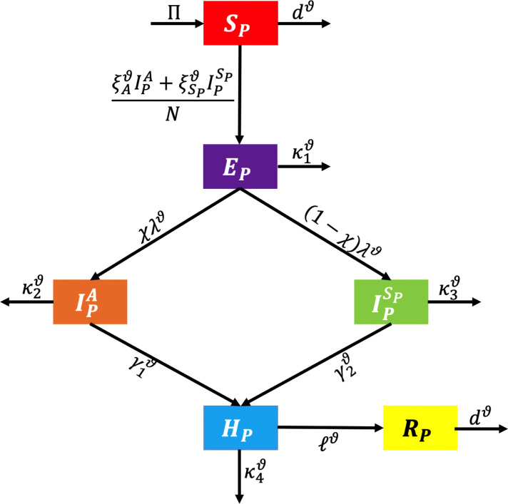
The model described here is an update of the SEIR model having two additional compartments. We propose an $\left(S_P{E}_P{I}_P^A{I}_P^{S_P}{H}_P{R}_P\right)$ constituent model, which contains the susceptible, exposed, infected (asymptomatic and symptomatic), hospitalized, and recovered population (see Fig. 1).

Fig. 1.

Flowchart of $\left(S_P{E}_P{I}_P^A{I}_P^{S_P}{H}_P{R}_P\right)$ model.

Because of this operator’s performance in simulating epidemic diseases and inspired by the practical applications of certain fractional operators in modeling such problems, in this paper, we are investigating the dynamics of the novel coronavirus model in the context of the nonlinear differential equation method involving the Atangana–Baleanu–Caputo (shortly, $ABC$) fractional derivative. Here, we give the following fractional system:

$$\left\{\begin{array}{cc}\hfill {}^{ABC}{\mathfrak{D}}_0^{\vartheta }{S}_P\left(t\right)& =\Pi -\frac{S_P\left(t\right)}{N}\left({\xi }_A^{\vartheta }{I}_P^A\left(t\right)+{\xi }_{S_P}^{\vartheta }{I}_P^{S_P}\left(t\right)\right)-d^{\vartheta }{S}_P\left(t\right),\hfill \\ \hfill {}^{ABC}{\mathfrak{D}}_0^{\vartheta }{E}_P\left(t\right)& =\frac{S_P\left(t\right)}{N}\left({\xi }_A^{\vartheta }{I}_P^A\left(t\right)+{\xi }_{S_P}^{\vartheta }{I}_P^{S_P}\left(t\right)\right)-\left({\lambda }^{\vartheta }+{\kappa }_1^{\vartheta }\right)E_P\left(t\right),\hfill \\ \hfill {}^{ABC}{\mathfrak{D}}_0^{\vartheta }{I}_P^A\left(t\right)& =\chi {\lambda }^{\vartheta }{E}_P\left(t\right)-\left({\gamma }_1^{\vartheta }+{\kappa }_2^{\vartheta }\right)I_P^A\left(t\right),\hfill \\ \hfill {}^{ABC}{\mathfrak{D}}_0^{\vartheta }{I}_P^S\left(t\right)& =\left(1-\chi \right){\lambda }^{\vartheta }{E}_P\left(t\right)-\left({\gamma }_2^{\vartheta }+{\kappa }_3^{\vartheta }\right)I_P^S\left(t\right),\hfill \\ \hfill {}^{ABC}{\mathfrak{D}}_0^{\vartheta }{H}_P\left(t\right)& ={\gamma }_1^{\vartheta }{I}_P^A\left(t\right)+{\gamma }_2^{\vartheta }{I}_P^S\left(t\right)-\left({\ell }^{\vartheta }+{\kappa }_4^{\vartheta }\right)H_P\left(t\right),\hfill \\ \hfill {}^{ABC}{\mathfrak{D}}_0^{\vartheta }{R}_P\left(t\right)& ={\ell }^{\vartheta }{H}_P\left(t\right)-d^{\vartheta }{R}_P\left(t\right),\hfill \end{array}\right)$$ (2.1)

with the initial conditions

$$\left\{\begin{array}{cc}\hfill S_P\left(0\right)& =S_{P0},\hfill \\ \hfill E_P\left(0\right)& =E_{P0},\hfill \\ \hfill I_P^A\left(0\right)& =I_{P0}^A,\hfill \\ \hfill I_P^{S_P}\left(0\right)& =I_{P0}^{S_P},\hfill \\ \hfill H_P\left(0\right)& =H_{P0},\hfill \\ \hfill R_P\left(0\right)& =R_{P0},\hfill \end{array}\right)$$ (2.2)

where $\Pi ≔n\times N,N$ is the total number of individuals and $n$ is the birth rate, ${}^{ABC}{\mathfrak{D}}_0^{\vartheta }$ denotes the $ABC$ fractional derivative of order $\vartheta \in [0,1)$ and all other parameters are described in Table 1. It is important to note that the model’s parameters are non-negative and having dimensions $\frac{1}{{\text{time}}^{\vartheta }}$.

Table 1.

Description of the parameters.

Parameter	Description
$d^{\vartheta }$	Death rate of individuals
${\xi }_A^{\vartheta },$${\xi }_{S_P}^{\vartheta }$	Transmission rates to the susceptible population from the asymptomatic and symptomatic populations, respectively
$\frac{1}{{\lambda }^{\vartheta }}$	Incubation period of an exposed individual
$\chi ,$$\left(1-\chi \right)$	Fraction of the exposed population that becomes asymptomatic after the incubation period and the remaining of the population are symptomatic, respectively
${\gamma }_1^{\vartheta },{\gamma }_2^{\vartheta }$	Infectious rates of an asymptomatic and a symptomatic individual, respectively
${\ell }^{\vartheta }$	Recovery rate through hospitalization
${\kappa }_1^{\vartheta },{\kappa }_2^{\vartheta },{\kappa }_3^{\vartheta },{\kappa }_4^{\vartheta }$	Mortality rates of the exposed, asymptomatic, symptomatic and hospitalized populations, respectively

The total population at time $t$ is $N$ which is further divided into $S_P\left(t\right),E_P\left(t\right),I_P^A\left(t\right)$, $I_P^{S_P}\left(t\right),H_P\left(t\right)$ and $R_P\left(t\right)$. The key assumptions are as follows:

• 1.natural mortality and birth rates are same;
• 2.the natural causes of death account for fatalities are presented in compartments $S_P$ and $R_P$;
• 3.the model’s death population is made up of individuals who died as a result of exposure ${\kappa }_1^{\vartheta }{E}_P\left(t\right)$, during infectious period (${\kappa }_2^{\vartheta }{I}_P^A\left(t\right)$ and ${\kappa }_3^{\vartheta }{I}_P^{S_P}\left(t\right)$) and hospitalization ${\kappa }_4^{\vartheta }{H}_P\left(t\right)$;
• 4.the total number of dead population from each compartment can be calculated by $\nu N≔d^{\vartheta }{S}_P+d^{\vartheta }{R}_P+{\kappa }_1^{\vartheta }{E}_P+{\kappa }_2^{\vartheta }{I}_P^A+{\kappa }_3^{\vartheta }{I}_P^{S_P}+{\kappa }_4^{\vartheta }{H}_P$;
• 5.other natural disasters have had a minimal effect on the population; therefore, we are neglecting them.

3. Auxiliary results

The following concepts and proven results would be needed in the sequel.

Definition 3.1 [35] —

Let $p\in [1,\infty )$ and $\mathfrak{O}$ be an open subset of $\mathbb{R}$, the Sobolev space $H^p\left(\mathfrak{O}\right)$ is defined by

$$H^p\left(\mathfrak{O}\right)=\{\Psi \in L^2\left(\mathfrak{O}\right):D^{\mu }\Psi \in L^2\left(\mathfrak{O}\right),\text{ for all }\left|\mu \right|\le p\}.$$

Based on the above definition, Atangana and Baleanu [9] gave the following definition of the Atangana–Baleanu fractional derivative in Caputo sense.

Definition 3.2 [9] —

Let $\Psi \in H^1(a,b)$, where $a,b\in \mathbb{R}$ with $a<b$, and $\vartheta \in [0,1)$. The Atangana and Baleanu fractional derivative in Caputo sense (shorten, $ABC$) are defined as follows:

$${}^{ABC}{\mathfrak{D}}_a^{\vartheta }\Psi \left(t\right)=\frac{\omega \left(\vartheta \right)}{1-\vartheta }{\int }_a^t\frac{d}{d\varsigma }\Psi \left(\varsigma \right){\mathbf{E}}_{\vartheta }\left[\frac{-\vartheta }{1-\vartheta }{(t-\varsigma )}^{\vartheta }\right]d\varsigma ,$$ (3.1)

where $\omega$ is the normalization function defined by $\omega \left(\vartheta \right)=\frac{\vartheta }{2-\vartheta }$, for all $0\le \vartheta <1$. Also, ${\mathbf{E}}_{\vartheta }$ stands for the Mittag-Leffler function which is a generalization of the exponential function (see [16], [23], [28]).

Remark 3.3

If we replace ${\mathbf{E}}_{\vartheta }\left[\frac{-\vartheta }{1-\vartheta }{(t-\varsigma )}^{\vartheta }\right]$ by ${\mathbf{E}}_1=exp\left[\frac{-\vartheta }{1-\vartheta }(t-\varsigma )\right]$, then we get the so-called Caputo–Fabrizio differential operator. Further, it is to be noted that

$${}^{ABC}{\mathfrak{D}}_0^{\vartheta }\left(\text{Constant}\right)=0.$$ (3.2)

Definition 3.4 [9] —

The Laplace transform of (3.1) is defined as follows:

$$\mathcal{L}\left\{{}^{ABC}{\mathfrak{D}}_a^{\vartheta }\Psi \left(t\right)\right\}\left(s\right)=\frac{\omega \left(\vartheta \right)}{1-\vartheta }\mathcal{L}\left[{\int }_a^t\Psi \left(\varsigma \right){\mathbf{E}}_{\vartheta }\left\{-\vartheta \frac{{(t-\varsigma )}^{\vartheta }}{1-\vartheta }\right\}d\varsigma \right]=\frac{\omega \left(\vartheta \right)}{1-\vartheta }\left[\frac{s^{\vartheta }\mathcal{L}\left\{\Psi \left(t\right)\right\}\left(s\right)-s^{\vartheta -1}\Psi \left(0\right)}{s^{\vartheta }+\frac{\vartheta }{1-\vartheta }}\right].$$ (3.3)

Definition 3.5 [9] —

Let $\Psi \in H^1(a,b)$, where $a,b\in \mathbb{R}$ with $a<b$, and $\vartheta \in [0,1)$. The corresponding integral in $ABC$ sense are defined as follows:

$${}^{ABC}{\mathbb{I}}_a^{\vartheta }\Psi \left(t\right)=\frac{1-\vartheta }{\omega \left(\vartheta \right)}\Psi \left(t\right)+\frac{\vartheta }{\omega \left(\vartheta \right)\Gamma \left(\vartheta \right)}{\int }_a^t{(t-\varsigma )}^{\vartheta -1}\Psi \left(\varsigma \right)d\varsigma ,$$ (3.4)

where $\Gamma$ is a gamma function.

Lemma 3.6

The solution of the given problem for$0\le \vartheta <1$,

$${}^{ABC}{\mathfrak{D}}_0^{\vartheta }\Psi \left(t\right)=\sigma \left(t\right),t\in [0,T],\Psi \left(0\right)={\Psi }_0,$$ (3.5)

where$\Psi :[0,T]\to \mathbb{R}$is an unknown function and${\Psi }_0$ is a fixed constant, provided by

$$\Psi \left(t\right)={\Psi }_0+\frac{1-\vartheta }{\omega \left(\vartheta \right)}\sigma \left(t\right)+\frac{\vartheta }{\omega \left(\vartheta \right)\Gamma \left(\vartheta \right)}{\int }_0^t{(t-\varsigma )}^{\vartheta -1}\sigma \left(\varsigma \right)d\varsigma .$$ (3.6)

For the qualitative analysis, we define the Banach space $\mathbb{F}=Y\times Y\times Y\times Y\times Y\times Y$, where $Y=C[0,T]$ with $0<T<\infty$, under the norm given for $\Psi ={\left({\psi }_1,{\psi }_2,{\psi }_3,{\psi }_4,{\psi }_5,{\psi }_6\right)}^T\in \mathbb{F}$ by

$$\Vert \Psi \Vert =\Vert {\left({\psi }_1,{\psi }_2,{\psi }_3,{\psi }_4,{\psi }_5,{\psi }_6\right)}^T\Vert =\underset{t\in [0,T]}{max}\left[\left|{\psi }_1\left(t\right)\right|+\left|{\psi }_2\left(t\right)\right|+\left|{\psi }_3\left(t\right)\right|+\left|{\psi }_4\left(t\right)\right|+\left|{\psi }_5\left(t\right)\right|+\left|{\psi }_6\left(t\right)\right|\right].$$

Throughout this paper, for $\mathbf{v}=(v_1,v_2,\dots ,v_6)\in {\mathbb{R}}^6$, we use this notion $\left|\cdot \right|$ as the taxicab norm in ${\mathbb{R}}^6$.

4. Existence and uniqueness of a solution

We shall examine the existence and uniqueness of a solution to our main model (2.1) with the condition (2.2) in this section. Let us write the model (2.1) with the condition (2.2) as

$$\left\{\begin{array}{cc}\hfill {}^{ABC}{\mathfrak{D}}_0^{\vartheta }{S}_P\left(t\right)& ={\Theta }_1\left(S_P\left(t\right),E_P\left(t\right),I_P^A\left(t\right),I_P^{S_P}\left(t\right),H_P\left(t\right),R_P\left(t\right)\right),\hfill \\ \hfill {}^{ABC}{\mathfrak{D}}_0^{\vartheta }{E}_P\left(t\right)& ={\Theta }_2\left(S_P\left(t\right),E_P\left(t\right),I_P^A\left(t\right),I_P^{S_P}\left(t\right),H_P\left(t\right),R_P\left(t\right)\right),\hfill \\ \hfill {}^{ABC}{\mathfrak{D}}_0^{\vartheta }{I}_P^A\left(t\right)& ={\Theta }_3\left(S_P\left(t\right),E_P\left(t\right),I_P^A\left(t\right),I_P^{S_P}\left(t\right),H_P\left(t\right),R_P\left(t\right)\right),\hfill \\ \hfill {}^{ABC}{\mathfrak{D}}_0^{\vartheta }{I}_P^{S_P}\left(t\right)& ={\Theta }_4\left(S_P\left(t\right),E_P\left(t\right),I_P^A\left(t\right),I_P^{S_P}\left(t\right),H_P\left(t\right),R_P\left(t\right)\right),\hfill \\ \hfill {}^{ABC}{\mathfrak{D}}_0^{\vartheta }{H}_P\left(t\right)& ={\Theta }_5\left(S_P\left(t\right),E_P\left(t\right),I_P^A\left(t\right),I_P^{S_P}\left(t\right),H_P\left(t\right),R_P\left(t\right)\right),\hfill \\ \hfill {}^{ABC}{\mathfrak{D}}_0^{\vartheta }{R}_P\left(t\right)& ={\Theta }_6\left(S_P\left(t\right),E_P\left(t\right),I_P^A\left(t\right),I_P^{S_P}\left(t\right),H_P\left(t\right),R_P\left(t\right)\right),\hfill \end{array}\right)$$ (4.1)

where

$$\left\{\begin{array}{cc}\hfill {\Theta }_1\left(S_P\left(t\right),E_P\left(t\right),I_P^A\left(t\right),I_P^{S_P}\left(t\right),H_P\left(t\right),R_P\left(t\right)\right)& =\Pi -\frac{S_P\left(t\right)}{N}\left({\xi }_A^{\vartheta }{I}_P^A\left(t\right)+{\xi }_{S_P}^{\vartheta }{I}_P^{S_P}\left(t\right)\right)\hfill \\ \hfill & -d^{\vartheta }{S}_P\left(t\right),\hfill \\ \hfill {\Theta }_2\left(S_P\left(t\right),E_P\left(t\right),I_P^A\left(t\right),I_P^{S_P}\left(t\right),H_P\left(t\right),R_P\left(t\right)\right)& =\frac{S_P\left(t\right)}{N}\left({\xi }_A^{\vartheta }{I}_P^A\left(t\right)+{\xi }_{S_P}^{\vartheta }{I}_P^{S_P}\left(t\right)\right)\hfill \\ \hfill & -\left({\lambda }^{\vartheta }+{\kappa }_1^{\vartheta }\right)E_P\left(t\right),\hfill \\ \hfill {\Theta }_3\left(S_P\left(t\right),E_P\left(t\right),I_P^A\left(t\right),I_P^{S_P}\left(t\right),H_P\left(t\right),R_P\left(t\right)\right)& =\chi {\lambda }^{\vartheta }{E}_P\left(t\right)-\left({\gamma }_1^{\vartheta }+{\kappa }_2^{\vartheta }\right)I_P^A\left(t\right),\hfill \\ \hfill {\Theta }_4\left(S_P\left(t\right),E_P\left(t\right),I_P^A\left(t\right),I_P^{S_P}\left(t\right),H_P\left(t\right),R_P\left(t\right)\right)& =\left(1-\chi \right){\lambda }^{\vartheta }{E}_P\left(t\right)-\left({\gamma }_2^{\vartheta }+{\kappa }_3^{\vartheta }\right)I_P^{{\mathcal{S}}_{\mathcal{P}}}\left(t\right),\hfill \\ \hfill {\Theta }_5\left(S_P\left(t\right),E_P\left(t\right),I_P^A\left(t\right),I_P^{S_P}\left(t\right),H_P\left(t\right),R_P\left(t\right)\right)& ={\gamma }_1^{\vartheta }{I}_P^A\left(t\right)+{\gamma }_2^{\vartheta }{I}_P^{S_P}\left(t\right)-\left({\ell }^{\vartheta }+{\kappa }_4^{\vartheta }\right)H_P\left(t\right),\hfill \end{array}\right)$$

$$\left\{\begin{array}{cc}\hfill {\Theta }_6\left(S_P\left(t\right),E_P\left(t\right),I_P^A\left(t\right),I_P^{S_P}\left(t\right),H_P\left(t\right),R_P\left(t\right)\right)& ={\ell }^{\vartheta }{H}_P\left(t\right)-d^{\vartheta }{R}_P\left(t\right)\hfill \end{array}\right)$$ (4.2)

with the condition (2.2). By using (2.1), we transform (4.2) with (2.2) to the following system:

$$\left\{\begin{array}{cc}\hfill {}^{ABC}{\mathfrak{D}}_0^{\vartheta }\Psi \left(t\right)& =\mathcal{Q}\left(t,\Psi \left(t\right)\right),\hfill \\ \hfill \Psi \left(0\right)& ={\Psi }_0,\hfill \end{array}\right)$$ (4.3)

where

$$\Psi =\left[\begin{array}{c}\hfill S_P\hfill \\ \hfill E_P\hfill \\ \hfill I_P^A\hfill \\ \hfill I_P^{S_P}\hfill \\ \hfill H_P\hfill \\ \hfill R_P\hfill \end{array}\right],{}^{ABC}{\mathfrak{D}}_0^{\vartheta }\Psi =\left[\begin{array}{c}\hfill {}^{ABC}{\mathfrak{D}}_0^{\vartheta }{S}_P\hfill \\ \hfill {}^{ABC}{\mathfrak{D}}_0^{\vartheta }{E}_P\hfill \\ \hfill {}^{ABC}{\mathfrak{D}}_0^{\vartheta }{I}_P^A\hfill \\ \hfill {}^{ABC}{\mathfrak{D}}_0^{\vartheta }{I}_P^{S_P}\hfill \\ \hfill {}^{ABC}{\mathfrak{D}}_0^{\vartheta }{H}_P\hfill \\ \hfill {}^{ABC}{\mathfrak{D}}_0^{\vartheta }{R}_P\hfill \end{array}\right],{\Psi }_0=\left[\begin{array}{c}\hfill S_{P0}\hfill \\ \hfill E_{P0}\hfill \\ \hfill I_{P0}^A\hfill \\ \hfill I_{P0}^{S_P}\hfill \\ \hfill H_{P0}\hfill \\ \hfill R_{P0}\hfill \end{array}\right],$$

and

$$\mathcal{Q}\left(t,\Psi \left(t\right)\right)=\left[\begin{array}{c}\hfill {\Theta }_1\left(S_P\left(t\right),E_P\left(t\right),I_P^A\left(t\right),I_P^{S_P}\left(t\right),H_P\left(t\right),R_P\left(t\right)\right)\hfill \\ \hfill {\Theta }_2\left(S_P\left(t\right),E_P\left(t\right),I_P^A\left(t\right),I_P^{S_P}\left(t\right),H_P\left(t\right),R_P\left(t\right)\right)\hfill \\ \hfill {\Theta }_3\left(S_P\left(t\right),E_P\left(t\right),I_P^A\left(t\right),I_P^{S_P}\left(t\right),H_P\left(t\right),R_P\left(t\right)\right)\hfill \\ \hfill {\Theta }_4\left(S_P\left(t\right),E_P\left(t\right),I_P^A\left(t\right),I_P^{S_P}\left(t\right),H_P\left(t\right),R_P\left(t\right)\right)\hfill \\ \hfill {\Theta }_5\left(S_P\left(t\right),E_P\left(t\right),I_P^A\left(t\right),I_P^{S_P}\left(t\right),H_P\left(t\right),R_P\left(t\right)\right)\hfill \\ \hfill {\Theta }_6\left(S_P\left(t\right),E_P\left(t\right),I_P^A\left(t\right),I_P^{S_P}\left(t\right),H_P\left(t\right),R_P\left(t\right)\right)\hfill \end{array}\right].$$

Using Lemma 3.6, the model (4.3) can be turned to the fractional integral equation in the sense of $ABC$ fractional integral as follows:

$$\Psi \left(t\right)={\Psi }_0+\frac{1-\vartheta }{\omega \left(\vartheta \right)}\mathcal{Q}\left(t,\Psi \left(t\right)\right)+\frac{\vartheta }{\omega \left(\vartheta \right)\Gamma \left(\vartheta \right)}{\int }_0^t{(t-\varsigma )}^{\vartheta -1}\mathcal{Q}\left(\varsigma ,\Psi \left(\varsigma \right)\right)d\varsigma .$$ (4.4)

Here we impose the following conditions:

• $\left({\Delta }_1\right)$
  there exist two constants $p_1>0$ and $p_2>0$ such that

  $$\left|\mathcal{Q}\left(t,\Psi \left(t\right)\right)\right|\le p_1\Vert \Psi \Vert +p_2,$$ (4.5)

  for all $t\in [0,T]$.
• $\left({\Delta }_2\right)$
  there exists $p_3>0$ such that

  $$|\mathcal{Q}\left(t,\Psi \left(t\right)\right)-\mathcal{Q}\left(t,\overline{\Psi }\left(t\right)\right)|\le p_3|\Psi \left(t\right)-\overline{\Psi }\left(t\right)|,$$ (4.6)

  for each $\Psi ,\overline{\Psi }\in \mathbb{F}$ and $t\in [0,T]$.

We start with the following result.

Lemma 4.1

The operator$\mathfrak{C\; :}$$\mathbb{F}\to \mathbb{F}$are defined in(4.4) is completely continuous.

Proof

First, we see that if $\Psi \in \mathbb{F}$, then $ℭ\Psi \in \mathbb{F}$. For each $\Psi \in D_Z≔\{\Psi \in \mathbb{F}:\Vert \Psi \Vert \le Z\}$, we obtain

$$\left|\left(ℭ\Psi \right)\left(t\right)\right|\le \Vert {\Psi }_0\Vert +\frac{1-\vartheta }{\omega \left(\vartheta \right)}\underset{t\in [0,1]}{max}\left|\mathcal{Q}\left(t,\Psi \left(t\right)\right)\right|+\underset{t\in [0,1]}{max}\frac{\vartheta }{\omega \left(\vartheta \right)\Gamma \left(\vartheta \right)}\times {\int }_0^t{(t-\varsigma )}^{\vartheta -1}\left|\mathcal{Q}\left(\varsigma ,\Psi \left(\varsigma \right)\right)\right|d\varsigma \le \Vert {\Psi }_0\Vert +\frac{1-\vartheta }{\omega \left(\vartheta \right)}\left(p_1\Vert \Psi \Vert +p_2\right)+\frac{\vartheta }{\omega \left(\vartheta \right)\Gamma \left(\vartheta \right)}{\int }_0^t{(t-\varsigma )}^{\vartheta -1}\left(p_1\Vert \Psi \Vert +p_2\right)d\varsigma \le \Vert {\Psi }_0\Vert +\left\{\frac{1-\vartheta }{\omega \left(\vartheta \right)}+\frac{T^{\vartheta }}{\omega \left(\vartheta \right)\Gamma \left(\vartheta \right)}\right\}{p}_2+\left\{\frac{1-\vartheta }{\omega \left(\vartheta \right)}+\frac{T^{\vartheta }}{\omega \left(\vartheta \right)\Gamma \left(\vartheta \right)}\right\}{p}_1\Vert \Psi \Vert \le \Vert {\Psi }_0\Vert +\Lambda \left(p_1\Vert \Psi \Vert +p_2\right)<+\infty ,$$

where $\Lambda ≔\left(\frac{1-\vartheta }{\omega \left(\vartheta \right)}+\frac{T^{\vartheta }}{\omega \left(\vartheta \right)\Gamma \left(\vartheta \right)}\right)$. This implies that

$$\Vert ℭ\Psi \Vert \le +\infty .$$

Hence, $ℭ$ is uniformly bounded on $D_Z$.

Next, we have to prove that the operator $ℭ$ is equicontinuous. For this, let $\Psi \in D_Z$ and $t_1,t_2\in [0,T]$ such that $t_1<t_2$. Then

$$|ℭ\Psi \left(t_2\right)-ℭ\Psi \left(t_1\right)|\le \frac{\vartheta }{\omega \left(\vartheta \right)\Gamma \left(\vartheta \right)}{\int }_{t_1}^{t_2}{(t_2-\varsigma )}^{\vartheta -1}\left|\mathcal{Q}\left(\varsigma ,\Psi \left(\varsigma \right)\right)\right|d\varsigma +\frac{\vartheta }{\omega \left(\vartheta \right)\Gamma \left(\vartheta \right)}{\int }_0^{t_1}\left\{{(t_2-\varsigma )}^{\vartheta -1}-{(t_1-\varsigma )}^{\vartheta -1}\right\}\left|\mathcal{Q}\left(\varsigma ,\Psi \left(\varsigma \right)\right)\right|d\varsigma$$

$$\le \frac{\left(p_{1}Z+p_2\right)}{\omega \left(\vartheta \right)\Gamma \left(\vartheta \right)}\left\{2{(t_2-t_1)}^{\vartheta }+(t_2^{\vartheta }-t_1^{\vartheta })\right\}.$$

Due to the fact that $t_1\to t_2$, the right hand side of the preceding inequality approaches to zero. As a result of the Arzelá–Ascoli theorem, $ℭ$ is compact and therefore completely continuous. □

Theorem 4.2

Assume that$\mathcal{Q}:[0,T]\times {\mathbb{R}}^6\to \mathbb{R}$is continuous and$\left({\Delta }_1\right)$ is satisfied. Then the integral Eq. (4.4) which is equivalent to the proposed COVID-19 model (2.1) – (2.2) has at least one solution.

Proof

Consider $\mathfrak{S}≔\{\Psi \in \mathbb{F}:\Psi =\delta \left(ℭ\Psi \right)\left(t\right),0<\delta <1\}$. From Lemma 4.1, it is clear that the operator $\mathfrak{C\; :}$ $\mathfrak{S}\to \mathbb{F}$ as given in (4.9) is completely continuous. From $\left({\Delta }_1\right)$, for any $\Psi \in \mathfrak{S}$, we obtain

$$\left|\Psi \left(t\right)\right|=\left|\delta \left(ℭ\Psi \right)\left(t\right)\right|\le \Vert {\Psi }_0\Vert +\frac{1-\vartheta }{\omega \left(\vartheta \right)}\left|\mathcal{Q}\left(t,\Psi \left(t\right)\right)\right|+\frac{\vartheta }{\omega \left(\vartheta \right)\Gamma \left(\vartheta \right)}{\int }_0^t{(t-\varsigma )}^{\vartheta -1}\left|\mathcal{Q}\left(\varsigma ,\Psi \left(\varsigma \right)\right)\right|d\varsigma \le \Vert {\Psi }_0\Vert +\frac{1-\vartheta }{\omega \left(\vartheta \right)}\left(p_1\Vert \Psi \Vert +p_2\right)+\frac{\vartheta }{\omega \left(\vartheta \right)\Gamma \left(\vartheta \right)}{\int }_0^t{(t-\varsigma )}^{\vartheta -1}\left(p_1\Vert \Psi \Vert +p_2\right)d\varsigma \le \Vert {\Psi }_0\Vert +\Lambda \left(p_2+p_1\Vert \Psi \Vert \right)<+\infty ,$$

where $\Lambda ≔\left(\frac{1-\vartheta }{\omega \left(\vartheta \right)}+\frac{T^{\vartheta }}{\omega \left(\vartheta \right)\Gamma \left(\vartheta \right)}\right)$. This implies that

$$\Vert \Psi \Vert \le +\infty .$$

As a result, $\mathfrak{S}$ is bounded. Hence, the operator has at least one fixed point, which happens to be the solution of the COVID-19 model (2.1)–(2.2). □

Theorem 4.3

Suppose that$\Psi \in \mathbb{F}$ and $\Psi$ maps a bounded subset of $[0,T]$ into relatively compact subset of ${\mathbb{R}}^6$ . Then the integral Eq. (4.4) which is equivalent to the proposed model (2.1) with the condition (2.2) has a unique solution provided that ${\tilde{\Lambda }}_1,\Lambda p_3<1$ , where

$$\Lambda ≔\left\{\frac{1-\vartheta }{\omega \left(\vartheta \right)}+\frac{T^{\vartheta }}{\omega \left(\vartheta \right)\Gamma \left(\vartheta \right)}\right\},$$ (4.7)

and

$${\tilde{\Lambda }}_1≔\left\{\frac{1-\vartheta }{\omega \left(\vartheta \right)}+\frac{T^{\vartheta }}{\omega \left(\vartheta \right)\Gamma \left(\vartheta \right)}\right\}{p}_1.$$ (4.8)

Proof

Let the operator $\mathfrak{C\; :}$ $\mathbb{F}\to \mathbb{F}$ defined for each $\Psi \in \mathbb{F}$ by

$$\left(ℭ\Psi \right)\left(t\right)={\Psi }_0+\frac{1-\vartheta }{\omega \left(\vartheta \right)}\mathcal{Q}\left(t,\Psi \left(t\right)\right)+\frac{\vartheta }{\omega \left(\vartheta \right)\Gamma \left(\vartheta \right)}{\int }_0^t{(t-\varsigma )}^{\vartheta -1}\mathcal{Q}\left(\varsigma ,\Psi \left(\varsigma \right)\right)d\varsigma ,$$ (4.9)

for all $t\in [0,T]$. It can be seen that the operator $ℭ$ is well defined and the unique solution of (4.9) is just the fixed point of $ℭ$. Here, we consider $D_Z=\{\Psi \in \mathbb{F}:\Vert \Psi \Vert \le Z\}$ as a closed and convex set with $Z\ge \frac{{\tilde{\Lambda }}_2}{1-{\tilde{\Lambda }}_1}$, where

$${\tilde{\Lambda }}_2≔\Vert {\Psi }_0\Vert +\left[\frac{1-\vartheta }{\omega \left(\vartheta \right)}+\frac{T^{\vartheta }}{\omega \left(\vartheta \right)\Gamma \left(\vartheta \right)}\right]p_2.$$ (4.10)

Thus, it is enough to show that $ℭD_Z\subset D_Z$. Now, for any $\Psi \in D_Z$, it yields

$$\left|\left(ℭ\Psi \right)\left(t\right)\right|\le \Vert {\Psi }_0\Vert +\frac{1-\vartheta }{\omega \left(\vartheta \right)}\left|\mathcal{Q}\left(t,\Psi \left(t\right)\right)\right|+\frac{\vartheta }{\omega \left(\vartheta \right)\Gamma \left(\vartheta \right)}{\int }_0^t{(t-\varsigma )}^{\vartheta -1}\left|\mathcal{Q}\left(\varsigma ,\Psi \left(\varsigma \right)\right)\right|d\varsigma \le \Vert {\Psi }_0\Vert +\frac{1-\vartheta }{\omega \left(\vartheta \right)}\left[p_1\Vert \Psi \Vert +p_2\right]+\frac{\vartheta }{\omega \left(\vartheta \right)\Gamma \left(\vartheta \right)}{\int }_0^t{(t-\varsigma )}^{\vartheta -1}\left[p_1\Vert \Psi \Vert +p_2\right]d\varsigma \le \Vert {\Psi }_0\Vert +\left[\frac{1-\vartheta }{\omega \left(\vartheta \right)}+\frac{T^{\vartheta }}{\omega \left(\vartheta \right)\Gamma \left(\vartheta \right)}\right]p_2+\left[\frac{1-\vartheta }{\omega \left(\vartheta \right)}+\frac{T^{\vartheta }}{\omega \left(\vartheta \right)\Gamma \left(\vartheta \right)}\right]p_{1}Z={\tilde{\Lambda }}_2+{\tilde{\Lambda }}_{1}Z\le Z.$$

Now, let ${\Psi }_1,{\Psi }_2\in \mathbb{F}$ and $t\in [0,T]$. Then, we obtain

$$|ℭ{\Psi }_1\left(t\right)-ℭ{\Psi }_2\left(t\right)|\le \frac{1-\vartheta }{\omega \left(\vartheta \right)}|\mathcal{Q}\left(\varsigma ,{\Psi }_1\left(\varsigma \right)\right)-\mathcal{Q}\left(\varsigma ,{\Psi }_2\left(\varsigma \right)\right)|+\frac{\vartheta }{\omega \left(\vartheta \right)\Gamma \left(\vartheta \right)}{\int }_0^t{(t-\varsigma )}^{\vartheta -1}|\mathcal{Q}\left(\varsigma ,{\Psi }_1\left(\varsigma \right)\right)-\mathcal{Q}\left(\varsigma ,{\Psi }_2\left(\varsigma \right)\right)|d\varsigma \le \left\{\frac{1-\vartheta }{\omega \left(\vartheta \right)}+\frac{T^{\vartheta }}{\omega \left(\vartheta \right)\Gamma \left(\vartheta \right)}\right\}{p}_3\Vert {\Psi }_1-{\Psi }_2\Vert =\Lambda p_3\Vert {\Psi }_1-{\Psi }_2\Vert .$$

This implies that

$$\Vert ℭ{\Psi }_1-ℭ{\Psi }_2\Vert \le \Lambda p_3\Vert {\Psi }_1-{\Psi }_2\Vert .$$

As $\Lambda p_3<1$, therefore $ℭ$ is a Banach contraction mapping. Hence, the integral Eq. (4.4) has a unique solution. Consequently, the proposed COVID-19 model (2.1)–(2.2) has a unique solution. □

5. Properties of the model

Here, we discuss some critical aspects of the model (2.1) or, more precisely, the system (4.3), including the boundedness and positivity of the solutions for $t\ge 0$.

5.1. Invariant region

The boundary of solutions for the nonlinear system (2.1) with non-negative initial conditions is determined in this subsection. Our major goal is to prove that the feasible region produced in ${\mathbb{R}}_{+}^6$ is positively invariant with respect to the fractional model (2.1).

Theorem 5.1

The feasible region of the proposed fractional model (2.1) is given by

$$\Omega ≔\left\{(S_P,E_P,I_P^A,I_P^{S_P},H_P,R_P)\in {\mathbb{R}}_{+}^6:0\le N\le \frac{\Pi }{\nu };S_P,E_P,I_P^A,I_P^{S_P},H_P,R_P\ge 0\right\}$$ (5.1)

The existence and uniqueness of the solution of model (2.1) have already been shown in the preceding section; all that remains is to demonstrate that the set $\Omega$ is positively invariant with respect to the condition (2.2). For the proof of Theorem 5.1, the following theorem will be utilized.

Theorem 5.2

The solutions of the system (2.1) are bounded.

Proof

To obtain the fractional derivative of total population, we add all the relations in system (2.1). So

$${}^{ABC}{\mathfrak{D}}_0^{\vartheta }N\left(t\right)={}^{ABC}{\mathfrak{D}}_0^{\vartheta }{S}_P\left(t\right)+{}^{ABC}{\mathfrak{D}}_0^{\vartheta }{E}_P\left(t\right)+{}^{ABC}{\mathfrak{D}}_0^{\vartheta }{I}_P^A\left(t\right)+{}^{ABC}{\mathfrak{D}}_0^{\vartheta }{I}_P^{S_P}\left(t\right)+{}^{ABC}{\mathfrak{D}}_0^{\vartheta }{H}_P\left(t\right)+{}^{ABC}{\mathfrak{D}}_0^{\vartheta }{R}_P=\Pi -d^{\vartheta }{S}_P\left(t\right)-d^{\vartheta }{R}_P\left(t\right)-{\kappa }_1^{\vartheta }{E}_P\left(t\right)-{\kappa }_2^{\vartheta }{I}_P^A\left(t\right)-{\kappa }_3^{\vartheta }{I}_P^{S_P}\left(t\right)-{\kappa }_4^{\vartheta }{H}_P\left(t\right)=\Pi -\nu N\left(t\right).$$ (5.2)

By applying the Laplace transform on both sides of above inequality, we obtain

$$\mathcal{L}\left\{{}^{ABC}{\mathfrak{D}}_0^{\vartheta }N\left(t\right)\right\}\left(s\right)=\frac{\Pi }{s}-\nu \mathcal{L}\left\{N\left(t\right)\right\}\left(s\right)$$

and then

$$\frac{\omega \left(\vartheta \right)s^{\vartheta }\mathcal{L}\left\{N\left(t\right)\right\}\left(s\right)}{\vartheta +(1-\vartheta )s^{\vartheta }}+\nu \mathcal{L}\left\{N\left(t\right)\right\}\left(s\right)=\Pi s^{\vartheta -(\vartheta +1)}+\frac{\omega \left(\vartheta \right)N\left(0\right)s^{\vartheta -1}}{\vartheta +(1-\vartheta )s^{\vartheta }},$$

where $N\left(0\right)$ represents the initial value of the total population and $\omega$ is the normalization function defined in Definition 3.2. This implies that

$$\mathcal{L}\left\{N\left(t\right)\right\}\left(s\right)=\frac{\Pi \left[(1-\vartheta )s^{\vartheta }+\vartheta \right]s^{\vartheta -(\vartheta +1)}+\omega \left(\vartheta \right)s^{\vartheta -1}N\left(0\right)}{\nu \vartheta +(1-\vartheta )s^{\vartheta }\vartheta +\omega \left(\vartheta \right)s^{\vartheta }}.$$

Now, by applying the inverse Laplace transform, we have

$$N\left(t\right)=\frac{\Pi \vartheta t^{\vartheta }}{(1-\vartheta )\nu +\omega \left(\vartheta \right)}{\mathbf{E}}_{\vartheta ,\vartheta +1}\left(-\wp t^{\vartheta }\right)+\left[\frac{\Pi (1-\vartheta )}{(1-\vartheta )\nu +\omega \left(\vartheta \right)}+\frac{\omega \left(\vartheta \right)N\left(0\right)}{\omega \left(\vartheta \right)+(1-\vartheta )\nu }{\mathbf{E}}_{\vartheta ,1}\left(-\wp t^{\vartheta }\right)\right],$$ (5.3)

where $\wp =\frac{\vartheta w}{\omega \left(\vartheta \right)+(1-\vartheta )\nu }$, and ${\mathbf{E}}_{a,b}$ is the Mittag-Leffler function with two parameters $a>0$ and $b>0$ may be defined by the following series

$${\mathbf{E}}_{a,b}(ħ)=\sum _{n=0}^{\infty }\frac{{ħ}^n}{\Gamma (an+b)},$$

whose Laplace transform is

$$\mathcal{L}\left\{t^{b-1}{\mathbf{E}}_{a,b}\left(\pm \Lambda t^a\right)\right\}=\frac{s^{a-b}}{s^a\mp \Lambda },$$

provided that $s>\mid \Lambda {\mid }^{1/a}$. For $a,b>0$, the Mittag-Leffler function satisfies

$${\mathbf{E}}_{a,b}(ħ)=\frac{1}{ħ}\left[{\mathbf{E}}_{a,b-a}(ħ)-\frac{1}{\Gamma (b-a)}\right],$$

and for the case $a=\vartheta ,b=\vartheta +1$ and $ħ=-\wp t^{\vartheta }$, we have

$${\mathbf{E}}_{\vartheta ,\vartheta +1}\left(-\wp t^{\vartheta }\right)=\frac{1}{\wp t^{\vartheta }}\left[1-{\mathbf{E}}_{\vartheta ,1}\left(-\wp t^{\vartheta }\right)\right].$$ (5.4)

From [9], it is clear that the Mittag-Leffler function is bounded for all $t>0$ and possess an asymptotic behavior. Therefore, from (5.2), (5.3), we can say that $N\left(t\right)\le \frac{\Pi }{\nu }$ as $t\to \infty$. Thus, $N\left(t\right)$ and all other variables of the model (2.1) are bounded in a region $\Omega$.

The solution remains $\mathbf{x}=0$ for all $t>0$ if ${\mathbf{x}}_{\mathbf{0}}=0$. Furthermore, for any non-negative set of initial conditions in $\Omega$, every solution of model (2.1) in

$${\mathbb{R}}_{+}^6=\left\{\mathbf{y}\in {\mathbb{R}}^6:\mathbf{y}\ge 0\right\},\mathbf{y}\left(t\right)={\left(S_P,E_P,I_P^A,I_P^{S_P},H_P,R_P\right)}^T,$$

approaches asymptotically in finite time $t$, enters and remains in $\Omega$. Thus, the closed set $\Omega$ is positively invariant for our system (2.1). □

5.2. Positivity of solutions

In this subsection, we will show that for all $t\ge 0$, the state variables $S_P,E_P,I_P^A,I_P^{S_P},H_P$ and $R_P$ are positive. This characteristic is essential in order to demonstrate that our model is physically feasible.

Theorem 5.3

The solution space $\left(S_P,E_P,I_P^A,I_P^{S_P},H_P,R_P\right)$ of the system (2.1) will remain positive forever with any non-negative initial data.

Proof

First equation of the model (2.1) is rearranged to give

$${}^{ABC}{\mathfrak{D}}_0^{\vartheta }{S}_P\left(t\right)\ge -\left(\frac{1}{N}\left({\xi }_A^{\vartheta }{I}_P^A\left(t\right)+{\xi }_{S_P}^{\vartheta }{I}_P^{S_P}\left(t\right)\right)+d^{\vartheta }\right)S_P\left(t\right).$$

As all the solutions are bounded, therefore, we let $\frac{I_P^A\left(t\right)}{N}$ and $\frac{I_P^{S_P}\left(t\right)}{N}$ are bounded by ${\rho }_1$ and ${\rho }_2$ respectively. Then,

$${}^{ABC}{\mathfrak{D}}_0^{\vartheta }{S}_P\left(t\right)\ge -q{S}_P\left(t\right),$$ (5.5)

where $q≔{\xi }_A^{\vartheta }{\rho }_1+{\xi }_{S_P}^{\vartheta }{\rho }_2+d^{\vartheta }$ is a constant. Applying the Laplace transform on both sides of (5.5), we obtain

$$\frac{\omega \left(\vartheta \right)s^{\vartheta }}{\vartheta +(1-\vartheta )s^{\vartheta }}\mathcal{L}\left\{S_P\left(t\right)\right\}\left(s\right)-\frac{\omega \left(\vartheta \right)s^{\vartheta }}{\vartheta +(1-\vartheta )s^{\vartheta }}{S}_P\left(0\right)\ge -q\mathcal{L}\left\{S_P\left(t\right)\right\}\left(s\right),$$

and

$$\mathcal{L}\left\{S_P\left(t\right)\right\}\left(s\right)\ge \frac{\omega \left(\vartheta \right)s^{\vartheta -1}{S}_P\left(0\right)}{\omega \left(\vartheta \right)+q(1-\vartheta )}\cdot \frac{s^{\vartheta -1}}{s^{\vartheta }+\frac{q\vartheta }{\omega \left(\vartheta \right)+q(1-\vartheta )}}.$$

Now, by applying the inverse Laplace transform, we have

$$S_P\left(t\right)\ge \frac{\omega \left(\vartheta \right)s^{\vartheta -1}{S}_P\left(0\right)}{\omega \left(\vartheta \right)+q(1-\vartheta )}{\mathbf{E}}_{\vartheta ,1}\left(-t^{\vartheta }\frac{q\vartheta }{\omega \left(\vartheta \right)+q(1-\vartheta )}\right).$$ (5.6)

Because both of the values on the right-hand side of (5.6) are positive. Therefore, for every $t\ge 0$, the solution $S_P\left(t\right)$ also remains positive. Likewise, for every $t\ge 0$ corresponding to any non-negative initial data, we can simply argue that $E_P>0,I_P^A>0,I_P^{S_P}>0,H_P>0,R_P>0$. As a result, the solutions in ${\mathbb{R}}_{+}^6$ will always be positive. □

5.3. Equilibrium points

Here, by solving the following system yields the equilibrium points of the suggested fractional model (2.1):

$${}^{ABC}{\mathfrak{D}}_0^{\vartheta }{S}_P={}^{ABC}{\mathfrak{D}}_0^{\vartheta }{E}_P={}^{ABC}{\mathfrak{D}}_0^{\vartheta }{I}_P^A={}^{ABC}{\mathfrak{D}}_0^{\vartheta }{I}_P^{S_P}={}^{ABC}{\mathfrak{D}}_0^{\vartheta }{H}_P={}^{ABC}{\mathfrak{D}}_0^{\vartheta }{R}_P=0.$$

The proposed model (2.1) has a unique non-negative Corona free equilibrium at the point after simple computations given by

$$E{P}_0^{\star }=\left(S_{P0}^{\star },E_{P0}^{\star },I_{P0}^{A\star },I_{P0}^{S_P\star },H_{P0}^{\star },R_{P0}^{\star }\right)=\left(\frac{\Pi }{\nu },0,0,0,0,0\right),$$

and a unique non-negative Corona present equilibrium at the point given by

$$E{P}_1^{\star }=\left(S_{P1}^{\star },E_{P1}^{\star },I_{P1}^{A\star },I_{P1}^{S_P\star },H_{P1}^{\star },R_{P1}^{\star }\right),$$

in the epidemiological region $\Omega$, where

$$S_{P1}^{\star }=\frac{S_{P0}^{\star }}{R_{P0}^{\star }}>0,$$

$$E_{P1}^{\star }=\left(\frac{R_{P0}^{\star }-1}{R_{P0}^{\star }}\right)\left(\frac{d^{\vartheta }{S}_{P0}^{\star }}{R_{P0}^{\star }\left({\lambda }^{\vartheta }+{\kappa }_1^{\vartheta }\right)}\right)>0,$$

$$I_{P1}^{A\star }=\left(\frac{R_{P0}^{\star }-1}{R_{P0}^{\star }}\right)\left(\frac{d^{\vartheta }\chi {\lambda }^{\vartheta }{S}_{P0}^{\star }}{R_{P0}^{\star }\left({\lambda }^{\vartheta }+{\kappa }_1^{\vartheta }\right)\left({\gamma }_1^{\vartheta }+{\kappa }_2^{\vartheta }\right)}\right)>0,$$

$$I_{P1}^{S_P\star }=\left(\frac{R_{P0}^{\star }-1}{R_{P0}^{\star }}\right)\left(\frac{d^{\vartheta }(1-\chi ){\lambda }^{\vartheta }{S}_{P0}^{\star }}{R_{P0}^{\star }\left({\lambda }^{\vartheta }+{\kappa }_1^{\vartheta }\right)\left({\gamma }_2^{\vartheta }+{\kappa }_3^{\vartheta }\right)}\right)>0,$$

$$H_{P1}^{\star }=\left(\frac{R_{P0}^{\star }-1}{R_{P0}^{\star }}\right)\left(\frac{d^{\vartheta }{\lambda }^{\vartheta }{S}_{P0}^{\star }}{R_{P0}^{\star }\left({\lambda }^{\vartheta }+{\kappa }_1^{\vartheta }\right)\left({\ell }_{\vartheta }^{\vartheta }+{\kappa }_4^{\vartheta }\right)}\right)\left(\frac{(1-\chi ){\gamma }_2^{\vartheta }}{{\gamma }_2^{\vartheta }+{\kappa }_3^{\vartheta }}+\chi \right)>0,$$

$$R_{P1}^{\star }=\left(\frac{R_{P0}^{\star }-1}{R_{P0}^{\star }}\right)\left(\frac{d^{\vartheta }{\ell }^{\vartheta }{\lambda }^{\vartheta }{S}_{P0}^{\star }}{R_{P0}^{\star }\left({\lambda }^{\vartheta }+{\kappa }_1^{\vartheta }\right)\left({\ell }_{\vartheta }^{\vartheta }+{\kappa }_4^{\vartheta }\right)}\right)\left(\frac{(1-\chi ){\gamma }_2^{\vartheta }}{{\gamma }_2^{\vartheta }+{\kappa }_3^{\vartheta }}+\chi \right)>0.$$

5.4. Threshold parameter ${\mathcal{R}}_0$

The value of the threshold parameter, commonly represented by ${\mathcal{R}}_0$, can be used to define the dynamics of mathematical models. Any infectious disease spreads when an infected individual comes into contact with a group of entirely susceptible persons. As a result, at the time $t\ge 0$, a threshold parameter refers to the total number of new infections created by an infected individual. It secretly predicts a model’s dynamical behavior, indicating that it gives more excellent knowledge regarding the disease’s future spread or containment.

The value of the threshold parameter in model (2.1) is determined using the conventional next generation matrix technique. If $\mathbf{v}=\left(v_1,v_2,v_3,v_4\right)={\left(E_P,I_P^A,I_P^{S_P},H_P\right)}^T\in {\mathbb{R}}_{+}^4$, then the model (2.1) can be written as

$${}^{ABC}{\mathfrak{D}}_0^{\vartheta }{\mathbf{v}}_i={\mathcal{F}}_i\left(\mathbf{v}\right)-{\mathcal{G}}_i\left(\mathbf{v}\right),i=1\left(1\right)4,$$

where ${\mathcal{F}}_i\left(\mathbf{v}\right)$ represents the rate of appearance of new infections in compartment $i$ and ${\mathcal{G}}_i\left(\mathbf{v}\right)$ denotes the rate of transfer of infections to and from compartment $i$.

Now, by taking the Jacobian of the matrices at point $E{P}_0^{\star }$, we have

$$\mathbf{F}=\left[\begin{array}{cccc}\hfill \frac{\partial {\mathcal{F}}_1}{\partial E_P}\hfill & \hfill \frac{\partial {\mathcal{F}}_1}{\partial I_P^A}\hfill & \hfill \frac{\partial {\mathcal{F}}_1}{\partial I_P^{S_P}}\hfill & \hfill \frac{\partial {\mathcal{F}}_1}{\partial H_P}\hfill \\ \hfill \frac{\partial {\mathcal{F}}_2}{\partial E_P}\hfill & \hfill \frac{\partial {\mathcal{F}}_2}{\partial I_P^A}\hfill & \hfill \frac{\partial {\mathcal{F}}_2}{\partial I_P^{S_P}}\hfill & \hfill \frac{\partial {\mathcal{F}}_2}{\partial H_P}\hfill \\ \hfill \frac{\partial {\mathcal{F}}_3}{\partial E_P}\hfill & \hfill \frac{\partial {\mathcal{F}}_3}{\partial I_P^A}\hfill & \hfill \frac{\partial {\mathcal{F}}_3}{\partial I_P^{S_P}}\hfill & \hfill \frac{\partial {\mathcal{F}}_3}{\partial H_P}\hfill \\ \hfill \frac{\partial {\mathcal{F}}_4}{\partial E_P}\hfill & \hfill \frac{\partial {\mathcal{F}}_4}{\partial I_P^A}\hfill & \hfill \frac{\partial {\mathcal{F}}_4}{\partial I_P^{S_P}}\hfill & \hfill \frac{\partial {\mathcal{F}}_4}{\partial H_P}\hfill \end{array}\right]=\left[\begin{array}{cccc}\hfill 0\hfill & \hfill {\xi }_A^{\vartheta }\hfill & \hfill {\xi }_{S_P}^{\vartheta }\hfill & \hfill 0\hfill \\ \hfill 0\hfill & \hfill 0\hfill & \hfill 0\hfill & \hfill 0\hfill \\ \hfill 0\hfill & \hfill 0\hfill & \hfill 0\hfill & \hfill 0\hfill \\ \hfill 0\hfill & \hfill 0\hfill & \hfill 0\hfill & \hfill 0\hfill \end{array}\right],$$

$$\mathbf{G}=\left[\begin{array}{cccc}\hfill \frac{\partial {\mathcal{G}}_1}{\partial E_P}\hfill & \hfill \frac{\partial {\mathcal{G}}_1}{\partial I_P^A}\hfill & \hfill \frac{\partial {\mathcal{G}}_1}{\partial I_P^{S_P}}\hfill & \hfill \frac{\partial {\mathcal{G}}_1}{\partial H_P}\hfill \\ \hfill \frac{\partial {\mathcal{G}}_2}{\partial E_P}\hfill & \hfill \frac{\partial {\mathcal{G}}_2}{\partial I_P^A}\hfill & \hfill \frac{\partial {\mathcal{G}}_2}{\partial I_P^{S_P}}\hfill & \hfill \frac{\partial {\mathcal{G}}_2}{\partial H_P}\hfill \\ \hfill \frac{\partial {\mathcal{G}}_3}{\partial E_P}\hfill & \hfill \frac{\partial {\mathcal{G}}_3}{\partial I_P^A}\hfill & \hfill \frac{\partial {\mathcal{G}}_3}{\partial I_P^{S_P}}\hfill & \hfill \frac{\partial {\mathcal{G}}_3}{\partial H_P}\hfill \\ \hfill \frac{\partial {\mathcal{G}}_4}{\partial E_P}\hfill & \hfill \frac{\partial {\mathcal{G}}_4}{\partial I_P^A}\hfill & \hfill \frac{\partial {\mathcal{G}}_4}{\partial I_P^{S_P}}\hfill & \hfill \frac{\partial {\mathcal{G}}_4}{\partial H_P}\hfill \end{array}\right]=\left[\begin{array}{cccc}\hfill {\lambda }^{\vartheta }+{\kappa }_1^{\vartheta }\hfill & \hfill 0\hfill & \hfill 0\hfill & \hfill 0\hfill \\ \hfill -{\lambda }^{\vartheta }\chi \hfill & \hfill {\gamma }_1^{\vartheta }+{\kappa }_2^{\vartheta }\hfill & \hfill 0\hfill & \hfill 0\hfill \\ \hfill -{\lambda }^{\vartheta }(1-\chi )\hfill & \hfill 0\hfill & \hfill {\gamma }_2^{\vartheta }+{\kappa }_3^{\vartheta }\hfill & \hfill 0\hfill \\ \hfill 0\hfill & \hfill -{\gamma }_1^{\vartheta }\hfill & \hfill -{\gamma }_2^{\vartheta }\hfill & \hfill {\ell }^{\vartheta }+{\kappa }_4^{\vartheta }\hfill \end{array}\right].$$

The maximum absolute eigenvalue of the positive matrix ${\mathbf{FG}}^{-1}$ is the value of ${\mathcal{R}}_0$ for the model (2.1). That is,

$${\mathcal{R}}_0=\frac{\left[\chi {\xi }_A^{\vartheta }\left({\gamma }_2^{\vartheta }+{\kappa }_3^{\vartheta }\right)+(1-\chi ){\xi }_{S_P}^{\vartheta }\left({\gamma }_1^{\vartheta }+{\kappa }_2^{\vartheta }\right)\right]{\lambda }^{\vartheta }}{\left({\lambda }^{\vartheta }+{\kappa }_1^{\vartheta }\right)\left({\gamma }_1^{\vartheta }+{\kappa }_2^{\vartheta }\right)\left({\gamma }_2^{\vartheta }+{\kappa }_3^{\vartheta }\right)}.$$

5.5. Strength number ${\mathcal{A}}_0$

The strength number is the expansion of the reproduction number. Without a doubt, the reproduction rate is critical in the study of epidemiology when it comes to the spread and extinction of diseases. The epidemiologist uses a variety of strategies to get such numbers (i.e., violation of the reproduction number’s uniqueness and many others). The primary conclusion of this strategy depends on the prediction of the waves of the transmission of illness. The essential point is that this number is evaluated using the next-generation matrix approach by assuming coronavirus-free equilibrium in the system (2.1) and calculating the second derivative of infectious classes. As a result, the transmission and transition matrices are denoted by F and G [8], respectively, where:

$$\tilde{\mathbf{F}}=\left[\begin{array}{cccc}\hfill \frac{{\partial }^2{\mathcal{F}}_1}{\partial E_P^2}\hfill & \hfill \frac{{\partial }^2{\mathcal{F}}_1}{\partial I_P^{A2}}\hfill & \hfill \frac{{\partial }^2{\mathcal{F}}_1}{\partial I_P^{S_{P}2}}\hfill & \hfill \frac{{\partial }^2{\mathcal{F}}_1}{\partial H_P^2}\hfill \\ \hfill \frac{{\partial }^2{\mathcal{F}}_2}{\partial E_P^2}\hfill & \hfill \frac{{\partial }^2{\mathcal{F}}_2}{\partial I_P^{A2}}\hfill & \hfill \frac{{\partial }^2{\mathcal{F}}_2}{\partial I_P^{S_{P}2}}\hfill & \hfill \frac{{\partial }^2{\mathcal{F}}_2}{\partial H_P^2}\hfill \\ \hfill \frac{{\partial }^2{\mathcal{F}}_3}{\partial E_P^2}\hfill & \hfill \frac{{\partial }^2{\mathcal{F}}_3}{{\partial }^2{I}_P^{A2}}\hfill & \hfill \frac{{\partial }^2{\mathcal{F}}_3}{\partial I_P^{S_{P}2}}\hfill & \hfill \frac{{\partial }^2{\mathcal{F}}_3}{\partial H_P^2}\hfill \\ \hfill \frac{{\partial }^2{\mathcal{F}}_4}{\partial E_P^2}\hfill & \hfill \frac{{\partial }^2{\mathcal{F}}_4}{{\partial }^2{I}_P^{A2}}\hfill & \hfill \frac{{\partial }^2{\mathcal{F}}_4}{{\partial }^2{I}_P^{S_{P}2}}\hfill & \hfill \frac{{\partial }^2{\mathcal{F}}_4}{\partial H_P^2}\hfill \end{array}\right]=\left[\begin{array}{cccc}\hfill 0\hfill & \hfill \frac{-{\xi }_A^{\vartheta }}{N^2}\hfill & \hfill \frac{-{\xi }_{S_P}^{\vartheta }}{N^2}\hfill & \hfill 0\hfill \\ \hfill 0\hfill & \hfill 0\hfill & \hfill 0\hfill & \hfill 0\hfill \\ \hfill 0\hfill & \hfill 0\hfill & \hfill 0\hfill & \hfill 0\hfill \\ \hfill 0\hfill & \hfill 0\hfill & \hfill 0\hfill & \hfill 0\hfill \end{array}\right].$$

Then

$$Det\left(\tilde{\mathbf{F}}{\mathbf{G}}^{-1}-\theta I_4\right)=0.$$

Hence, the strength number ${\mathcal{A}}_0$ is

$${\mathcal{A}}_0=\left(\frac{-{\lambda }^{\vartheta }}{N^2}\right)\left[\frac{\left(\chi {\xi }_A^{\vartheta }\left({\gamma }_2^{\vartheta }+{\kappa }_3^{\vartheta }\right)+(1-\chi ){\xi }_{S_P}^{\vartheta }\left({\gamma }_1^{\vartheta }+{\kappa }_2^{\vartheta }\right)\right)}{\left({\lambda }^{\vartheta }+{\kappa }_1^{\vartheta }\right)\left({\gamma }_1^{\vartheta }+{\kappa }_2^{\vartheta }\right)\left({\gamma }_2^{\vartheta }+{\kappa }_3^{\vartheta }\right)}\right]<0.$$

A negative strength number indicates that the system (2.1) will have a single magnitude, either a maximum with two infection sites suggesting a single wave or a quick drop from the coronavirus-free equilibrium. As a result, the infection will grow to a minimal point with the renewal process, then stabilize or halt as requested later.

6. Stability results

The consistency of solutions has a strong emphasis on the theory of mathematical modeling. For illustration, slight variations in the model, induced by natural measurement errors in practical situations, have a minor proportional impact on the solution. The mathematical calculations that explain the system will not accurately forecast the probable result. Hence, the stability of the suggested mathematical model (2.1) with ((2.2) ) must be discussed here. For the detail of the Ulam–Hyers and generalized Ulam–Hyers stability, we refer [6], [19], [40], [41].

The definitions that follow are required in the upcoming results. Let $\epsilon >0$ and consider the following inequality:

$$|{}^{ABC}{\mathfrak{D}}_0^{\vartheta }\tilde{\Psi }\left(t\right)-\mathcal{Q}\left(t,\tilde{\Psi }\left(t\right)\right)|\le \epsilon ,t\in [0,T],$$ (6.1)

where $\epsilon =max{\left({\epsilon }_j\right)}^T$, $j=1,2,\dots ,6$.

Definition 6.1

The proposed problem (3.5), which is equivalent to model (2.1)–(2.2), is Ulam–Hyers stable if there exists $\Xi >0$ such that, for every $\epsilon >0$ and for each solution $\tilde{\Psi }\in \mathbb{F}$ satisfying inequality (6.1), there exists a solution $\Psi \in \mathbb{F}$ of problem (4.3) with the initial condition $\tilde{\Psi }\left(0\right)=\Psi \left(0\right)$ such that 

$$|\tilde{\Psi }\left(t\right)-\Psi \left(t\right)|\le \Xi \epsilon ,t\in [0,T],$$

where

$$\tilde{\Psi }=\left[\begin{array}{c}\hfill {\tilde{S}}_P\hfill \\ \hfill {\tilde{E}}_P\hfill \\ \hfill {\tilde{I}}_P^A\hfill \\ \hfill {\tilde{I}}_P^{S_P}\hfill \\ \hfill {\tilde{H}}_P\hfill \\ \hfill {\tilde{R}}_P\hfill \end{array}\right],{\tilde{\Psi }}_0=\left[\begin{array}{c}\hfill {\tilde{S}}_{P0}\hfill \\ \hfill {\tilde{E}}_{P0}\hfill \\ \hfill {\tilde{I}}_{P0}^A\hfill \\ \hfill {\tilde{I}}_{P0}^{S_P}\hfill \\ \hfill cvskip\left[3pt\right]{\tilde{H}}_{P0}\hfill \\ \hfill {\tilde{R}}_{P0}\hfill \end{array}\right],\Xi =max\left[\begin{array}{c}\hfill {\Xi }_1\hfill \\ \hfill {\Xi }_2\hfill \\ \hfill {\Xi }_3\hfill \\ \hfill {\Xi }_4\hfill \\ \hfill {\Xi }_5\hfill \\ \hfill {\Xi }_6\hfill \end{array}\right],\epsilon =max\left[\begin{array}{c}\hfill {\epsilon }_1\hfill \\ \hfill {\epsilon }_2\hfill \\ \hfill {\epsilon }_3\hfill \\ \hfill {\epsilon }_4\hfill \\ \hfill {\epsilon }_5\hfill \\ \hfill {\epsilon }_6\hfill \end{array}\right],$$

and

$$\mathcal{Q}\left(t,\tilde{\Psi }\left(t\right)\right)=\left[\begin{array}{c}\hfill {\tilde{\Theta }}_1\left({\tilde{S}}_P\left(t\right),{\tilde{E}}_P\left(t\right),{\tilde{I}}_P^A\left(t\right),{\tilde{I}}_P^{S_P}\left(t\right),{\tilde{H}}_P\left(t\right),{\tilde{R}}_P\left(t\right)\right)\hfill \\ \hfill {\tilde{\Theta }}_2\left({\tilde{S}}_P\left(t\right),{\tilde{E}}_P\left(t\right),{\tilde{I}}_P^A\left(t\right),{\tilde{I}}_P^{S_P}\left(t\right),{\tilde{H}}_P\left(t\right),{\tilde{R}}_P\left(t\right)\right)\hfill \\ \hfill {\tilde{\Theta }}_3\left({\tilde{S}}_P\left(t\right),{\tilde{E}}_P\left(t\right),{\tilde{I}}_P^A\left(t\right),{\tilde{I}}_P^{S_P}\left(t\right),{\tilde{H}}_P\left(t\right),{\tilde{R}}_P\left(t\right)\right)\hfill \\ \hfill {\tilde{\Theta }}_4\left({\tilde{S}}_P\left(t\right),{\tilde{E}}_P\left(t\right),{\tilde{I}}_P^A\left(t\right),{\tilde{I}}_P^{S_P}\left(t\right),{\tilde{H}}_P\left(t\right),{\tilde{R}}_P\left(t\right)\right)\hfill \\ \hfill {\tilde{\Theta }}_5\left({\tilde{S}}_P\left(t\right),{\tilde{E}}_P\left(t\right),{\tilde{I}}_P^A\left(t\right),{\tilde{I}}_P^{S_P}\left(t\right),{\tilde{H}}_P\left(t\right),{\tilde{R}}_P\left(t\right)\right)\hfill \\ \hfill {\tilde{\Theta }}_6\left({\tilde{S}}_P\left(t\right),{\tilde{E}}_P\left(t\right),{\tilde{I}}_P^A\left(t\right),{\tilde{I}}_P^{S_P}\left(t\right),{\tilde{H}}_P\left(t\right),{\tilde{R}}_P\left(t\right)\right)\hfill \end{array}\right].$$

Definition 6.2

Problem (4.3), which is equivalent to the model (2.1) with (2.2), is referred to as being generalized Ulam–Hyers stable if there exists a continuous function $\phi :{\mathbb{R}}^{+}\to {\mathbb{R}}^{+}$ with $\phi \left(0\right)=0$ such that for each solution $\tilde{\Psi }\in \mathbb{F}$ of the inequality (6.1), there exists a solution $\Psi \in \mathbb{F}$ of Problem (4.3) such that

$$|\tilde{\Psi }\left(t\right)-\Psi \left(t\right)|\le \phi \epsilon ,t\in [0,T],$$

where $\phi =max{\left({\phi }_j\right)}^T$, $j=1,2,\dots ,6$.

Assumption 6.3

Consider a small perturbation $h\in C[0,T]$ such that $h\left(0\right)=0$ with the following properties:

• (i)$\left|h\left(t\right)\right|\le \epsilon$, $h=max{\left(h_j\right)}^T$, $t\in [0,T]$ and $\epsilon >0;$
• (ii)
  for $t\in [0,T]$, we have the following model

  $${}^{ABC}{\mathfrak{D}}_0^{\vartheta }\tilde{\Psi }\left(t\right)=\mathcal{Q}\left(t,\tilde{\Psi }\left(t\right)\right)+h\left(t\right),$$

  where $h\left(t\right)={(h_1\left(t\right),h_2\left(t\right),\dots ,h_6\left(t\right))}^T$.

Lemma 6.4

The solution of the perturbed problem

$$\left\{\begin{array}{cc}\hfill {}^{ABC}{\mathfrak{D}}_0^{\vartheta }\tilde{\Psi }\left(t\right)& =\mathcal{Q}\left(t,\tilde{\Psi }\left(t\right)\right)+h\left(t\right),\hfill \\ \hfill \tilde{\Psi }\left(0\right)& ={\tilde{\Psi }}_0,\hfill \end{array}\right)$$ (6.2)

satisfies the given relation

$$|{\tilde{\Psi }}_h\left(t\right)-\tilde{\Psi }\left(t\right)|\le \Lambda \epsilon ,$$

where${\tilde{\Psi }}_h\left(t\right)$is a solution of(6.2),$\tilde{\Psi }\left(t\right)$ satisfies (6.1) and $\Lambda ≔\left(\frac{1-\vartheta }{\omega \left(\vartheta \right)}+\frac{T^{\vartheta }}{\omega \left(\vartheta \right)\Gamma \left(\vartheta \right)}\right)$ .

Proof

In view of $\left(ii\right)$ of Assumption 6.3 and Lemma 3.6, the solution of (6.2) is given by

$${\tilde{\Psi }}_h\left(t\right)={\tilde{\Psi }}_0+\frac{1-\vartheta }{\omega \left(\vartheta \right)}\mathcal{Q}\left(t,\tilde{\Psi }\left(t\right)\right)+\frac{\vartheta }{\omega \left(\vartheta \right)\Gamma \left(\vartheta \right)}{\int }_0^t{(t-\varsigma )}^{\vartheta -1}\mathcal{Q}\left(t,\tilde{\Psi }\left(\varsigma \right)\right)d\varsigma +\frac{1-\vartheta }{\omega \left(\vartheta \right)}h\left(t\right)+\frac{\vartheta }{\omega \left(\vartheta \right)\Gamma \left(\vartheta \right)}{\int }_0^t{(t-\varsigma )}^{\vartheta -1}h\left(\varsigma \right)d\varsigma .$$

Furthermore, we have

$$\tilde{\Psi }\left(t\right)={\tilde{\Psi }}_0+\frac{1-\vartheta }{\omega \left(\vartheta \right)}\mathcal{Q}\left(t,\tilde{\Psi }\left(t\right)\right)+\frac{\vartheta }{\omega \left(\vartheta \right)\Gamma \left(\vartheta \right)}{\int }_0^t{(t-\varsigma )}^{\vartheta -1}\mathcal{Q}\left(t,\tilde{\Psi }\left(\varsigma \right)\right)d\varsigma .$$

Using $\left(i\right)$ of Assumption 6.3, we get

$$|{\tilde{\Psi }}_h\left(t\right)-\tilde{\Psi }\left(t\right)|\le \frac{1-\vartheta }{\omega \left(\vartheta \right)}\left|h\left(t\right)\right|+\frac{\vartheta }{\omega \left(\vartheta \right)\Gamma \left(\vartheta \right)}{\int }_0^t{(t-\varsigma )}^{\vartheta -1}\left|h\left(\varsigma \right)\right|d\varsigma \le \left(\frac{1-\vartheta }{\omega \left(\vartheta \right)}+\frac{T^{\vartheta }}{\omega \left(\vartheta \right)\Gamma \left(\vartheta \right)}\right)\epsilon =\Lambda \epsilon ,$$

where $\Lambda ≔\left(\frac{1-\vartheta }{\omega \left(\vartheta \right)}+\frac{T^{\vartheta }}{\omega \left(\vartheta \right)\Gamma \left(\vartheta \right)}\right)$.

This implies that

$$|{\tilde{\Psi }}_h\left(t\right)-\tilde{\Psi }\left(t\right)|\le \Lambda \epsilon .$$

Hence, we get the desired result. □

Theorem 6.5

Under the assumptions of Theorem 4.3 , the model (2.1) – (2.2) is Ulam–Hyers and, consequently, generalized Ulam–Hyers stable.

Proof

Suppose that $\tilde{\Psi }\in \mathbb{F}$ satisfies inequality (6.1) and $\Psi \in \mathbb{F}$ is a unique solution of problem (4.4) with the condition

$$\Psi \left(0\right)=\tilde{\Psi }\left(0\right).$$ (6.3)

Due to (6.3), we can write (4.4) as

$$\Psi \left(t\right)=\tilde{\Psi }\left(0\right)+\frac{1-\vartheta }{\omega \left(\vartheta \right)}\mathcal{Q}\left(t,\Psi \left(t\right)\right)+\frac{\vartheta }{\omega \left(\vartheta \right)\Gamma \left(\vartheta \right)}{\int }_0^t{(t-\varsigma )}^{\vartheta -1}\mathcal{Q}\left(\varsigma ,\Psi \left(\varsigma \right)\right)d\varsigma .$$

Thus, by (${\Delta }_1$)  and Lemma 6.4, we obtain

$$|\tilde{\Psi }\left(t\right)-\Psi \left(t\right)|\le |\tilde{\Psi }\left(t\right)-{\tilde{\Psi }}_h\left(t\right)|+|{\tilde{\Psi }}_h\left(t\right)-\Psi \left(t\right)|\le \Lambda \epsilon +\frac{1-\vartheta }{\omega \left(\vartheta \right)}|\mathcal{Q}\left(t,\tilde{\Psi }\left(t\right)\right)-\mathcal{Q}\left(t,\Psi \left(t\right)\right)|+\Lambda \epsilon +\frac{\vartheta }{\omega \left(\vartheta \right)\Gamma \left(\vartheta \right)}{\int }_0^t{(t-\varsigma )}^{\vartheta -1}|\mathcal{Q}\left(t,\tilde{\Psi }\left(t\right)\right)-\mathcal{Q}\left(t,\Psi \left(t\right)\right)|d\varsigma$$

$$\le 2\Lambda \epsilon +\left(\frac{1-\vartheta }{\omega \left(\vartheta \right)}+\frac{T^{\vartheta }}{\omega \left(\vartheta \right)\Gamma \left(\vartheta \right)}\right)p_3\Vert \tilde{\Psi }-\Psi \Vert =2\Lambda \epsilon +\Lambda p_3\Vert \tilde{\Psi }-\Psi \Vert .$$

Hence,

$$\Vert \tilde{\Psi }-\Psi \Vert \le \frac{2\Lambda \epsilon }{1-\Lambda p_3}.$$

As, $\Lambda p_3<1$, we obtain

$$\Vert \tilde{\Psi }-\Psi \Vert \le \Xi \epsilon ,$$

where $\Xi ≔$ $\frac{2\Lambda }{1-\Lambda p_3}$. □

Remark 6.6

If we set $\phi \left(\epsilon \right)=\Xi \epsilon$ such that $\phi \left(0\right)=0$, then from the above theorem, we conclude that the proposed model (2.1) with (2.2) is generalized Ulam–Hyers stable.

7. Numerical simulations and discussion

In this section, we need to examine the estimated solutions of the $ABC$ fractional-order model (2.1) with (2.2). The theoretical models are then obtained by employing the current scheme. The $ABC$ fractional derivative is utilized to develop the computational procedure for the simulation of our model (2.1).

7.1. General algorithm

In this subsection, we offer a numerical technique for analyzing and predicting the numerical stability of a Coronavirus fractional model (2.1) with (2.2) based on a recently developed Toufik–Atangana criterion [36]. We first outline the concept briefly before applying it to the fractional model (2.1) with (2.2) to get an iterative approach. The system (2.1) may be represented using the fundamental theorem of fractional calculus.

$$z\left(t\right)-z\left(0\right)=\frac{1-\vartheta }{\omega \left(\vartheta \right)}\Psi (t,z\left(t\right))+\frac{\vartheta }{\omega \left(\vartheta \right)\Gamma \left(\vartheta \right)}{\int }_0^t{(t-\varsigma )}^{\vartheta -1}\Psi (\varsigma ,z\left(\varsigma \right))d\varsigma ,$$

At $t=t_{n+1},n=0,1,2,\dots ,N$ with $h=\frac{T}{N}$, we have

$$z\left(t_{n+1}\right)=z\left(0\right)+\frac{1-\vartheta }{\omega \left(\vartheta \right)}\Psi (t_n,z\left(t_n\right))+\frac{\vartheta }{\omega \left(\vartheta \right)\Gamma \left(\vartheta \right)}\sum _{j=0}^n{\int }_{t_j}^{t_{j+1}}{(t_{n+1}-\varsigma )}^{\vartheta -1}\Psi (\varsigma ,z\left(\varsigma \right))d\varsigma .$$ (7.1)

The function $\Psi (\varsigma ,z\left(\varsigma \right))$ can be approximated over $\left[t_j,t_{j+1}\right]$, using the interpolation polynomial

$$\Psi (\varsigma ,z\left(\varsigma \right))=\frac{\Psi (t_j,z\left(t_j\right))}{h}\times (t-t_{j-1})-\frac{\Psi (t_{j-1},z\left(t_{j-1}\right))}{h}\times (t-t_j).$$

By substituting this in (7.1), we obtain

$$z\left(t_{n+1}\right)=z\left(0\right)+\frac{1-\vartheta }{\omega \left(\vartheta \right)}\Psi (t_n,z\left(t_n\right))+\frac{\vartheta }{\omega \left(\vartheta \right)\Gamma \left(\vartheta \right)}\sum _{j=0}^n\left[\frac{\Psi (t_j,z\left(t_j\right))}{h}\times \right)\left({\int }_{t_j}^{t_{j+1}}{(t_{n+1}-t)}^{\vartheta -1}(t-t_{j-1})dt-\frac{\Psi (t_{j-1},z\left(t_{j-1}\right))}{h}{\int }_{t_j}^{t_{j+1}}{(t_{n+1}-t)}^{\vartheta -1}(t-t_j)dt\right].$$

Finally, we get the approximate solution as:

$$z\left(t_{n+1}\right)=z\left(t_0\right)+\frac{1-\vartheta }{\omega \left(\vartheta \right)}\Psi (t_n,z\left(t_n\right))+\frac{\vartheta }{\omega \left(\vartheta \right)}\sum _{j=0}^n\left[\frac{h^{\vartheta }\Psi (t_j,z\left(t_j\right))}{\Gamma (\vartheta +2)}\times \right)\left\{(n-j+2+\vartheta ){(n+1-j)}^{\vartheta }(n-j+2+2\vartheta ){(n-j)}^{\vartheta }\right\}-\left(\frac{h^{\vartheta }\Psi (t_{j-1},z\left(t_{j-1}\right))}{\Gamma (\vartheta +2)}\left\{{(n+1-j)}^{\vartheta +1}-(n-j+1+\vartheta ){(n-j)}^{\vartheta }\right\}\right].$$

Hence, we obtain the following recursive formula for the model equations:

$$\left\{\begin{array}{cc}\hfill S_P\left(t_{n+1}\right)& =S_P\left(t_0\right)+\frac{1-\vartheta }{\omega \left(\vartheta \right)}{\Psi }_1(t_n,z\left(t_n\right))+\frac{\vartheta }{\omega \left(\vartheta \right)}\sum _{j=0}^n\left[\frac{h^{\vartheta }{\Psi }_1(t_j,z\left(t_j\right))}{\Gamma (\vartheta +2)}\times \right)\hfill \\ \hfill & \left\{(n-j+2+\vartheta ){(n+1-j)}^{\vartheta }(n-j+2+2\vartheta ){(n-j)}^{\vartheta }\right\}\hfill \\ \hfill & -\left(\frac{h^{\vartheta }{\Psi }_1(t_{j-1},z\left(t_{j-1}\right))}{\Gamma (\vartheta +2)}\left\{{(n+1-j)}^{\vartheta +1}-(n-j+1+\vartheta ){(n-j)}^{\vartheta }\right\}\right],\hfill \\ \hfill E_P\left(t_{n+1}\right)& =E_P\left(t_0\right)+\frac{1-\vartheta }{\omega \left(\vartheta \right)}{\Psi }_2(t_n,z\left(t_n\right))+\frac{\vartheta }{\omega \left(\vartheta \right)}\sum _{j=0}^n\left[\frac{h^{\vartheta }{\Psi }_2(t_j,z\left(t_j\right))}{\Gamma (\vartheta +2)}\times \right)\hfill \\ \hfill & \left\{(n-j+2+\vartheta ){(n+1-j)}^{\vartheta }(n-j+2+2\vartheta ){(n-j)}^{\vartheta }\right\}\hfill \\ \hfill & -\left(\frac{h^{\vartheta }{\Psi }_1(t_{j-1},z\left(t_{j-1}\right))}{\Gamma (\vartheta +2)}\left\{{(n+1-j)}^{\vartheta +1}-(n-j+1+\vartheta ){(n-j)}^{\vartheta }\right\}\right],\hfill \end{array}\right)$$

$$\left\{\begin{array}{cc}\hfill I_P^A\left(t_{n+1}\right)& =I_P^A\left(t_0\right)+\frac{1-\vartheta }{\omega \left(\vartheta \right)}{\Psi }_3(t_n,z\left(t_n\right))+\frac{\vartheta }{\omega \left(\vartheta \right)}\sum _{j=0}^n\left[\frac{h^{\vartheta }{\Psi }_3(t_j,z\left(t_j\right))}{\Gamma (\vartheta +2)}\times \right)\hfill \\ \hfill & \left\{(n-j+2+\vartheta ){(n+1-j)}^{\vartheta }(n-j+2+2\vartheta ){(n-j)}^{\vartheta }\right\}\hfill \\ \hfill & -\left(\frac{h^{\vartheta }{\Psi }_1(t_{j-1},z\left(t_{j-1}\right))}{\Gamma (\vartheta +2)}\left\{{(n+1-j)}^{\vartheta +1}-(n-j+1+\vartheta ){(n-j)}^{\vartheta }\right\}\right],\hfill \\ \hfill I_P^{S_P}\left(t_{n+1}\right)& =I_P^{S_P}\left(t_0\right)+\frac{1-\vartheta }{\omega \left(\vartheta \right)}{\Psi }_4(t_n,z\left(t_n\right))+\frac{\vartheta }{\omega \left(\vartheta \right)}\sum _{j=0}^n\left[\frac{h^{\vartheta }{\Psi }_4(t_j,z\left(t_j\right))}{\Gamma (\vartheta +2)}\times \right)\hfill \\ \hfill & \left\{(n-j+2+\vartheta ){(n+1-j)}^{\vartheta }(n-j+2+2\vartheta ){(n-j)}^{\vartheta }\right\}\hfill \\ \hfill & -\left(\frac{h^{\vartheta }{\Psi }_1(t_{j-1},z\left(t_{j-1}\right))}{\Gamma (\vartheta +2)}\left\{{(n+1-j)}^{\vartheta +1}-(n-j+1+\vartheta ){(n-j)}^{\vartheta }\right\}\right],\hfill \\ \hfill H_P\left(t_{n+1}\right)& =H_P\left(t_0\right)+\frac{1-\vartheta }{\omega \left(\vartheta \right)}{\Psi }_5(t_n,z\left(t_n\right))+\frac{\vartheta }{\omega \left(\vartheta \right)}\sum _{j=0}^n\left[\frac{h^{\vartheta }{\Psi }_5(t_j,z\left(t_j\right))}{\Gamma (\vartheta +2)}\times \right)\hfill \\ \hfill & \left\{(n-j+2+\vartheta ){(n+1-j)}^{\vartheta }(n-j+2+2\vartheta ){(n-j)}^{\vartheta }\right\}\hfill \\ \hfill & -\left(\frac{h^{\vartheta }{\Psi }_1(t_{j-1},z\left(t_{j-1}\right))}{\Gamma (\vartheta +2)}\left\{{(n+1-j)}^{\vartheta +1}-(n-j+1+\vartheta ){(n-j)}^{\vartheta }\right\}\right],\hfill \\ \hfill R_P\left(t_{n+1}\right)& =R_P\left(t_0\right)+\frac{1-\vartheta }{\omega \left(\vartheta \right)}{\Psi }_6(t_n,z\left(t_n\right))+\frac{\vartheta }{\omega \left(\vartheta \right)}\sum _{j=0}^n\left[\frac{h^{\vartheta }{\Psi }_6(t_j,z\left(t_j\right))}{\Gamma (\vartheta +2)}\times \right)\hfill \\ \hfill & \left\{(n-j+2+\vartheta ){(n+1-j)}^{\vartheta }(n-j+2+2\vartheta ){(n-j)}^{\vartheta }\right\}\hfill \\ \hfill & -\left(\frac{h^{\vartheta }{\Psi }_1(t_{j-1},z\left(t_{j-1}\right))}{\Gamma (\vartheta +2)}\left\{{(n+1-j)}^{\vartheta +1}-(n-j+1+\vartheta ){(n-j)}^{\vartheta }\right\}\right].\hfill \end{array}\right)$$ (7.2)

7.2. Results and discussion

This portion includes a computational simulation of the transmission dynamics of COVID-19 in society. To this end, the initial conditions are posited as $S_P\left(0\right)=600,I_P^A\left(0\right)=90,and{I}_P^{S_P}\left(0\right)=40$. Here, for the model’s parameters, we choose ${\xi }_A^{\vartheta }=1\times 10^{-10},{\xi }_{S_P}^{\vartheta }=1.2312,{\lambda }^{\vartheta }=9.9618\times 10^{-3},{\kappa }_1^{\vartheta }=3.3491\times 10^{-3},{\kappa }_2^{\vartheta }=1\times 10^{-10},{\kappa }_3^{\vartheta }=3.0859\times 10^{-4},{\kappa }_4^{\vartheta }=2.1222\times 10^{-5},\chi =1.5683\times 10^{-1},{\gamma }_1^{\vartheta }=2.6628\times 10^{-2},{\gamma }_2^{\vartheta }=1,{\ell }^{\vartheta }=6.170\times 10^{-3}$.

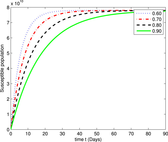
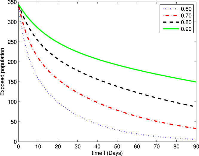
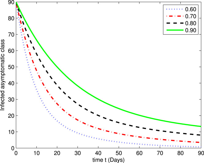
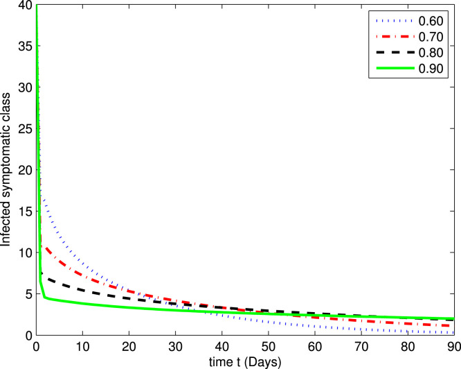
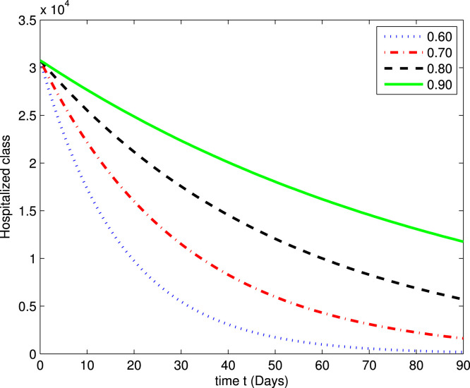
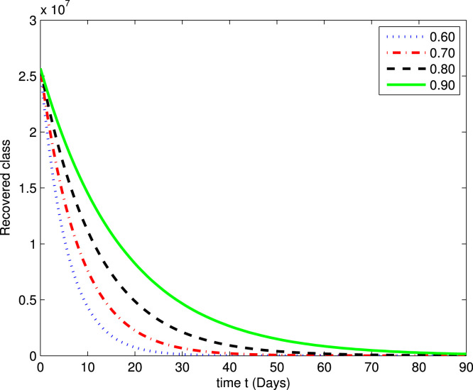
In the following Fig. 2, Fig. 3, Fig. 4, Fig. 5, Fig. 6, Fig. 7, by using a MATLAB package, we create an algorithm to simulate the effects of different parameters corresponding to various fractional values of $\vartheta$. We presented numerical data of $90$ days. As you can see in Fig. 2, Fig. 3, Fig. 4, Fig. 5, Fig. 6, Fig. 7, the parameters have different impacts but demonstrate the same behavior in different proportions of $\vartheta$. Fig. 2, Fig. 3 indicate that over time $t$, $S_P\left(t\right)$, and $E_P\left(t\right)$ (increase and decrease) hit the equilibrium point. It means the susceptible individuals will expand over time, while the exposed population will decline. It is apparent from Fig. 4, Fig. 5 that, with time, the affected community (asymptomatic ${\mathcal{I}}_P^A\left(t\right)$ and symptomatic $I_P^{S_P}\left(t\right)$) hits their stable points. As COVID-19 infection cases initially rose, the amount of hospitalized patients $H_P\left(t\right)$ was higher (as seen in Fig. 6), although it would decrease with time. Also, the number of COVID-19 contaminated classes decreases over time; therefore, the recovered class $R_P\left(t\right)$ eventually decreases (see Fig. 7).

Fig. 2.

The graph illustrating the approximate solution for the susceptible class $\left(S_P\right)$ at different fractional values of $\vartheta$.

Fig. 3.

The graph illustrating the approximate solution for the exposed class $\left(E_P\right)$ at different fractional values of $\vartheta$.

Fig. 4.

The graph illustrating the approximate solution for the infected asymptomatic class $\left(I_P^A\right)$ at different fractional values of $\vartheta$.

Fig. 5.

The graph illustrating the approximate solution for the infected symptomatic class $\left(I_P^{S_P}\right)$ at different fractional values of $\vartheta$.

Fig. 6.

The graph illustrating the approximate solution for the hospitalized class $\left(H_P\right)$ at different fractional values of $\vartheta$.

Fig. 7.

The graph illustrating the approximate solution for the recovered class $\left(R_P\right)$ at different fractional values of $\vartheta$.

8. Conclusion

In this work, we developed a fractional-order $\left(S_P{E}_P{I}_P^A{I}_P^{S_P}{H}_P{R}_P\right)$ model to examine the dynamics of a new Coronavirus infection. We employed the Atangana–Baleanu derivative operator with the generalized Mittag-Leffler function to formulate the suggested fractional model. Due to its non-local and non-singular kernel, the Atangana–Baleanu derivative operator was selected. Our study’s objective was to concentrate on an $\left(S_P{E}_P{I}_P^A{I}_P^{S_P}{H}_P{R}_P\right)$ model that accurately depicted the predominant properties of the Coronavirus. The fixed point theorems were used to verify the existence and uniqueness of the solution to the suggested fractional model. The basic reproduction number and strength number were calculated theoretically and numerically to account for the model’s dynamical behavior. Also, we developed some results about the qualitative theory and Ulam–Hyers stability analysis. Additionally, we calculated numerical solutions for the given model using an efficient method. Graphic representations had created to verify the dynamic behavior of the solution using Matlab. The results collected are critical in explaining the present dynamics of the COVID-19 epidemic. Moreover, it can be seen that the fractional calculus can explain the population’s dynamics more concisely. The studies reported may be more efficient with the current outbreak and use preventive measures to mitigate infection. The suggested framework may be utilized in the future to explore other nonlinear fractional differential problems using the $ABC$ fractional derivative.

Declaration of Competing Interest

The authors declare that they have no known competing financial interests or personal relationships that could have appeared to influence the work reported in this paper.

Availability of data and materials

Data sharing not applicable to this article as no datasets were generated or analyzed during the current study.

References

- 1.Abdeljawad T., Agarwal R.P., Karapınar E., Kumari P.S. Solutions of the nonlinear integral equation and fractional differential equation using the technique of a fixed point with a numerical experiment in extended b-metric space. Symmetry. 2019;11(5):686. [Google Scholar]
- 2.Adhanom T., et al. 2020. World health organization director-general’s opening remarks at the media briefing on COVID-19—11 March 2020. World Healt h Organization. [Google Scholar]
- 3.Adiguzel R.S., Aksoy U., Karapinar E., Erhan I.M. On the solutions of fractional differential equations via geraghty type hybrid contractions. Appl. Comput. Math. 2021;20(2):313–333. [Google Scholar]
- 4.Afshari H., Karapınar E. A discussion on the existence of positive solutions of the boundary value problems via -hilfer fractional derivative on b-metric spaces. Adv. Differ. Equ. 2020;2020(1):1–11. [Google Scholar]
- 5.Ali W., Turab A., Nieto J.J. On the novel existence results of solutions for a class of fractional boundary value problems on the cyclohexane graph. J. Inequal. Appl. 2022;2022(1):1–19. [Google Scholar]
- 6.Alqahtani B., Fulga A., Karapınar E. Fixed point results on -symmetric quasi-metric space via simulation function with an application to Ulam stability. Mathematics. 2018;6(10):208. [Google Scholar]
- 7.Anderson R.M., May R.M. Population biology of infectious diseases: part I. Nature. 1979;280(5721):361–367. doi: 10.1038/280361a0. [DOI] [PubMed] [Google Scholar]
- 8.Atangana A. 2021. Mathematical model of survival of fractional calculus, critics and their impact: how singular is our world? [Google Scholar]
- 9.Atangana A., Baleanu D. 2016. New fractional derivatives with nonlocal and non-singular kernel: theory and application to heat transfer model. arXiv preprint arXiv:1602.03408. [Google Scholar]
- 10.Baleanu D., Jajarmi A., Hajipour M. On the nonlinear dynamical systems within the generalized fractional derivatives with Mittag–Leffler kernel. Nonlinear dyn. 2018;94(1):397–414. [Google Scholar]
- 11.Brauer F., Castillo-Chavez C., Castillo-Chavez C. Springer; 2012. Mathematical Models in Population Biology and Epidemiology, vol.2. [Google Scholar]
- 12.Caputo M., Fabrizio M. A new definition of fractional derivative without singular kernel. Progr. Fract. Differ. Appl. 2015;1(2):1–13. [Google Scholar]
- 13.Caputo M., Mainardi F. A new dissipation model based on memory mechanism. Pure appl. Geophys. 1971;91(1):134–147. [Google Scholar]
- 14.Fernandez A., Baleanu D., Srivastava H. Series representations for fractional-calculus operators involving generalised mittag-leffler functions. Commun. Nonlinear Sci. Numer. Simul. 2019;67:517–527. [Google Scholar]
- 15.Gorbalenya A.E., Baker S.C., Baric R., Groot R.J.d., Drosten C., Gulyaeva A.A., Haagmans B.L., Lauber C., Leontovich A.M., Neuman B.W., et al. 2020. Severe acute respiratory syndrome-related coronavirus: the species and its viruses–a statement of the coronavirus study group. [Google Scholar]
- 16.Hilfer R. World scientific; 2000. Applications of fractional calculus in physics. [Google Scholar]
- 17.Ivorra B., Martínez-López B., Sánchez-Vizcaíno J.M., Ramos Á.M. Mathematical formulation and validation of the be-fast model for classical swine fever virus spread between and within farms. Ann. oper. res. 2014;219(1):25–47. [Google Scholar]
- 18.Jajarmi A., Baleanu D. A new fractional analysis on the interaction of HIV with CD4+ T-cells. Chaos Solitons Fract. 2018;113:221–229. [Google Scholar]
- 19.Karapınar E., Fulga A. An admissible hybrid contraction with an ulam type stability. Demonstratio Math. 2019;52(1):428–436. [Google Scholar]
- 20.Koca I. Analysis of rubella disease model with non-local and non-singular fractional derivatives. Int. J. Optim. Control Theor. Appl. (IJOCTA) 2018;8(1):17–25. [Google Scholar]
- 21.Kucharski A.J., Russell T.W., Diamond C., Liu Y., Edmunds J., Funk S., Eggo R.M., Sun F., Jit M., Munday J.D., et al. Early dynamics of transmission and control of COVID-19: a mathematical modelling study. lancet infect. dis. 2020;20(5):553–558. doi: 10.1016/S1473-3099(20)30144-4. [DOI] [PMC free article] [PubMed] [Google Scholar]
- 22.Kumar D., Singh J. New aspects of fractional epidemiological model for computer viruses with mittag–leffler law. Math. Model. Health Soc. Appl. Sci. (Springer, Singapore, 2020) 2020:283–301. [Google Scholar]
- 23.Lakshmikantham V., Leela S., Devi J.V. 2009. Theory of fractional dynamic systems. Cambridge Sci Publ., Cambridge. [Google Scholar]
- 24.Lazarević M.P., Spasić A.M. Finite-time stability analysis of fractional order time-delay systems: gronwall’s approach. Math. Comput. Model. 2009;49(3-4):475–481. [Google Scholar]
- 25.Li R., Pei S., Chen B., Song Y., Zhang T., Yang W., Shaman J. Substantial undocumented infection facilitates the rapid dissemination of novel coronavirus (SARS-CoV-2) Science. 2020;368(6490):489–493. doi: 10.1126/science.abb3221. [DOI] [PMC free article] [PubMed] [Google Scholar]
- 26.Martínez-López B., Ivorra B., Ramos A., Sánchez-Vizcaíno J.M. A novel spatial and stochastic model to evaluate the within-and between-farm transmission of classical swine fever virus. i. general concepts and description of the model. Vet. microbiol. 2011;147(3-4):300–309. doi: 10.1016/j.vetmic.2010.07.009. [DOI] [PubMed] [Google Scholar]
- 27.Organization W.H., et al. Naming the coronavirus disease (COVID-19) and the virus that causes it. Br. J. Implantol. Health Sci. 2020;2(3) [Google Scholar]
- 28.Podlubny I. Academic press; New York: 1999. Fractional Differential Equations, Mathematics in Science and Engineering. [Google Scholar]
- 29.Qureshi S., Yusuf A., Shaikh A.A., Inc M., Baleanu D. Fractional modeling of blood ethanol concentration system with real data application. Chaos Interdiscip. J. Nonlinear Sci. 2019;29(1):013143. doi: 10.1063/1.5082907. [DOI] [PubMed] [Google Scholar]
- 30.Roosa K., Lee Y., Luo R., Kirpich A., Rothenberg R., Hyman J., Yan P., Chowell G.b. Real-time forecasts of the covid-19 epidemic in china from february 5th to february 24th, 2020. Infect. Dis. Model. 2020;5:256–263. doi: 10.1016/j.idm.2020.02.002. [DOI] [PMC free article] [PubMed] [Google Scholar]
- 31.Sevinik Adigüzel R., Aksoy Ü., Karapinar E., Erhan İ.M. On the solution of a boundary value problem associated with a fractional differential equation. Math. Methods Appl. Sci. 2020 [Google Scholar]
- 32.Sevinik Adigüzel R., Aksoy Ü., Karapinar E., Erhan İ.M. On the solution of a boundary value problem associated with a fractional differential equation. Math. Methods Appl. Sci. 2020 [Google Scholar]
- 33.Sevinik-Adıgüzel R., Aksoy Ü., Karapınar E., Erhan İ.M. Uniqueness of solution for higher-order nonlinear fractional differential equations with multi-point and integral boundary conditions. Rev. Real Acad. Ciencias Exactas, Físicas y Nat. Ser. A. 2021;115(3):1–16. [Google Scholar]
- 34.Sintunavarat W., Turab A. On the novel existence results of solutions for fractional langevin equation associating with nonlinear fractional orders. Thai J. Math. 2021;19(3):827–841. [Google Scholar]
- 35.Syam M., Al-Refai M. Fractional differential equations with Atangana–Baleanu fractional derivative: analysis and applications. Chaos Solitons Fract. X. 2019;2:100013. [Google Scholar]
- 36.Toufik M., Atangana A. New numerical approximation of fractional derivative with non-local and non-singular kernel: application to chaotic models. Eur. Phys. J. Plus. 2017;132(10):1–16. [Google Scholar]
- 37.Turab A., Mitrović Z.D., Savić A. Existence of solutions for a class of nonlinear boundary value problems on the hexasilinane graph. Adv. Differ. Equ. 2021;2021(1):1–20. [Google Scholar]
- 38.Turab A., Sintunavarat W. The novel existence results of solutions for a nonlinear fractional boundary value problem on the ethane graph. Alex. Eng. J. 2021;60(6):5365–5374. [Google Scholar]
- 39.Uçar S. Amer Inst Mathematical Sciences-AIMS; 2020. Analysis of a Basic SEIRA Model with Atangana-Baleanu Derivative. [Google Scholar]
- 40.Ulam S.M. Interscience Publishers; 1960. A Collection of Mathematical Problems. [Google Scholar]
- 41.Ulam S.M. Courier Corporation; 2004. Problems in Modern Mathematics. [Google Scholar]
- 42.Wang C., Horby P.W., Hayden F.G., Gao G.F. A novel coronavirus outbreak of global health concern. lancet. 2020;395(10223):470–473. doi: 10.1016/S0140-6736(20)30185-9. [DOI] [PMC free article] [PubMed] [Google Scholar]
- 43.Wang Y., Wang Y., Chen Y., Qin Q. Unique epidemiological and clinical features of the emerging 2019 novel coronavirus pneumonia (covid-19) implicate special control measures. J. med. virol. 2020;92(6):568–576. doi: 10.1002/jmv.25748. [DOI] [PMC free article] [PubMed] [Google Scholar]
- 44.World Health Organization, (2005) Y., et al. 2020. Statement on the second meeting of the international health regulations (2005) emergency committee regarding the outbreak of novel coronavirus (2019-nCoV) [Google Scholar]
- 45.Yan D., Cao H. The global dynamics for an age-structured tuberculosis transmission model with the exponential progression rate. Appl. Math. Model. 2019;75:769–786. [Google Scholar]
Associated Data
This section collects any data citations, data availability statements, or supplementary materials included in this article.
Data Availability Statement