Machine Learning Models of Arsenic in Private Wells Throughout the Conterminous United States As a Tool for Exposure Assessment in Human Health Studies

Abstract

Arsenic from geologic sources is widespread in groundwater within the United States (U.S.). In several areas, groundwater arsenic concentrations exceed the U.S. Environmental Protection Agency maximum contaminant level of 10 μg per liter (μg/L). However, this standard applies only to public-supply drinking water and not to private-supply, which is not federally regulated and is rarely monitored. As a result, arsenic exposure from private wells is a potentially substantial, but largely hidden, public health concern. Machine learning models using boosted regression trees (BRT) and random forest classification (RFC) techniques were developed to estimate probabilities and concentration ranges of arsenic in private wells throughout the conterminous U.S. Three BRT models were fit separately to estimate the probability of private well arsenic concentrations exceeding 1, 5, or 10 μg/L whereas the RFC model estimates the most probable category ≤5, >5 to ≤10, or >10 μg/ L). Overall, the models perform best at identifying areas with low concentrations of arsenic in private wells. The BRT 10 μg/L model estimates for testing data have an overall accuracy of 91.2%, sensitivity of 33.9%, and specificity of 98.2%. Influential variables identified across all models included average annual precipitation and soil geochemistry. Models were developed in collaboration with public health experts to support U.S.-based studies focused on health effects from arsenic exposure.

Graphical Abstract

INTRODUCTION

Worldwide, it is estimated that more than 200 million people are chronically exposed to arsenic from drinking water at concentrations greater than 10 μg per liter (μg/L), the World Health Organization (WHO) drinking water quality guideline.^1,2 Contaminated drinking water remains a major route of exposure^3,4 and a particular concern for vulnerable subpopulations, such as infants, children, the elderly, and those with compromised immune systems.^5,6 Arsenic is more prevalent in drinking water from groundwater sources than from surface water supplies, and in groundwater its occurrence is typically attributed to geogenic sources.⁷

Through studying exposed populations, arsenic has been associated with an increased risk of adverse health consequences across multiple organ systems,⁸ with evidence of pathological effects on the pulmonary,^9,10 cardiovascular,^11,12 reproductive,¹³ immune,^14,15 nervous,¹⁶ and endocrine systems,¹⁷ as well as the skin,^18,19 liver,^20,21 kidney,²² and bladder.^23,24 Multiple lines of evidence suggest a connection between chronic arsenic exposure and cancer and impaired child development.^3,25–30

In 2001, the U.S. Environmental Protection Agency (EPA) lowered the maximum contaminant level (MCL) for arsenic in public water supplies from 50 μg/L to 10 μg/L based on an extensive review of available information including WHO drinking water quality guidelines.^2,5,6,31 EPA MCLs are enforceable drinking water standards based on health-related data as well as technical and economic feasibility considerations.⁶ In addition to MCLs, the EPA promulgates nonenforceable MCL goals (MCLGs),⁶ based exclusively on public health and defined as the threshold level at which no risk to public health is expected. The EPA MCLG for arsenic is zero.^5,6

Some U.S. states and other countries have enacted more stringent MCLs for arsenic. In the U.S., New Jersey has adopted an MCL of 5 μg/L, and New Hampshire has proposed an MCL of 5 μg/L to take effect in July 2021.^32,33 Internationally, Denmark has an MCL of 5 μg/L,³⁴ and water utilities in The Netherlands have a water quality goal for arsenic of less than 1 μg/L.³⁵

The health consequences of chronic arsenic exposure have primarily been identified from populations who were exposed to drinking water concentrations greatly exceeding the WHO and EPA recommended level of 10 μg/L.^9,11,16 However, several epidemiological studies suggest that low-level exposure to arsenic near or below 10 μg/L may also increase the risk of arsenic-associated diseases.^{12,24,36–39}

Approximately 40 million Americans living in agricultural, rural, or other low population areas rely on private-supply wells for drinking water, wells that supply ≤24 people or ≤14 hookups, and typically serve a single household.^40–42 The EPA is not authorized to monitor or regulate private wells under the Safe Drinking Water Act,⁴³ and owner self-monitoring is rare^44,45 due to high analytical costs and unfounded belief in taste and odor as a reliable indicator of safety.^44–47 Local public health departments often require a water quality test for private wells upon transfer of ownership; however, it is typically limited to bacteria or nitrate and rarely includes arsenic or other contaminants. Arsenic is one of the most common contaminants (including all geogenic and anthropogenically sourced inorganic or organic contaminants) detected above the MCL in private wells throughout the U.S.^45,48,49 In two national studies of thousands of private wells, arsenic exceeded the 10 μg/L MCL in 10.6% and 6.75% of the wells and exceeded the MCLG of zero (reported above 1 μg/L) in 51% and 46% of private wells.^45,48 For comparison other inorganic contaminants frequently detected above the drinking water MCL include uranium (4%) and nitrate (8%), with organic contaminants rarely exceeding MCLs.^45,48,49 These and other similar findings have resulted in focused attention on the role that arsenic plays in degrading the quality of private well water and its role in human health outcomes. Understanding arsenic occurrence in private wells is important for understanding human health effects associated with this generally unmonitored arsenic exposure pathway. The development of robust models that produce maps estimating the likelihood of arsenic occurrence on a national level is a critical first step in evaluating adverse health effects of arsenic intake from private well water in the U.S.

Historically, methods such as logistic regression (LR) models have been used to estimate the spatial occurrence of arsenic in groundwater and to identify areas with elevated concentrations at local,^50,51 regional,^52–55 national,^56–61 and global⁶² scales. LR models assume linear relationships between dependent and independent model variables and are not wellsuited for predictor variable collinearity.⁶³ Some studies have used modified or combined methods to address these linearity constraints.⁶² Further, the geochemical reactions and hydrologic circumstances that result in elevated arsenic levels are complex⁷ and unlikely to be well-described by linear models across large geographic areas. Machine learning methods can capture complex patterns in data⁶⁴ and are promising alternatives to linear models for estimating groundwater quality. Machine learning techniques that have been used to model groundwater arsenic include random forest,^65–67 hybrid random forest,⁶⁸ boosted regression trees,^51,69 and classification and regression trees (CART).⁷⁰

The current study builds upon previous research, which employed LR to estimate the population exposed to private-well arsenic concentrations greater than 10 μg/L throughout the conterminous U.S. (CONUS).⁵⁸ Here, we developed three boosted regression tree (BRT) models to separately estimate the probability of arsenic concentrations exceeding 1, 5, and 10 μg/L and a single random forest classification (RFC) model to estimate the most likely arsenic concentration category (≤5, >5 to ≤10, or >10 μg/L) in private wells throughout the CONUS.

The main aim of this study was to develop national scale models to provide consistent estimates of the probability of exceeding arsenic concentration thresholds and to develop the models for comparison to national scale human health data. As such, we developed maps of groundwater arsenic in private wells at the CONUS scale, with input from epidemiologists and public-health scientists, so that large, scale-compatible linkages can be made between potential arsenic exposures at greater than 1, 5, and 10 μg/L and existing data quantifying adverse human-health outcomes. Although the models and human health data may have variable amounts of uncertainty, these models and maps provide previously unavailable information, especially in sparsely sampled areas, and will enable geospatial comparisons of high and low potential arsenic exposure to frequent and infrequent occurrence of adverse human health conditions. In this way, arsenic exposure estimates can be used to evaluate relations between potential exposure and adverse human outcomes for a variety of diseases.

METHODS

Arsenic Concentrations in Private Wells.

Private well locations and associated arsenic concentrations used in this study are as described previously for LR modeling.⁵⁸ Arsenic concentrations from a total of 20 450 private wells were available from samples collected between 1970 and 2013.⁷¹ Samples were collected prior to passing through water treatment systems, if any were present. Well locations and applicable model(s) are shown in Figure 1. Arsenic concentration reporting limits varied from <0.5 to 10 μg/L, with a total of 9293 wells (45%) containing concentrations below a reporting limit (Table SI_1). Due to the prevalence of wells with arsenic concentrations reported below a reporting limit, categorical or threshold concentration models were developed that estimate a probability of exceeding a concentration threshold or occurring within a concentration range, rather than regression models that estimate a concentration value.

Figure 1.

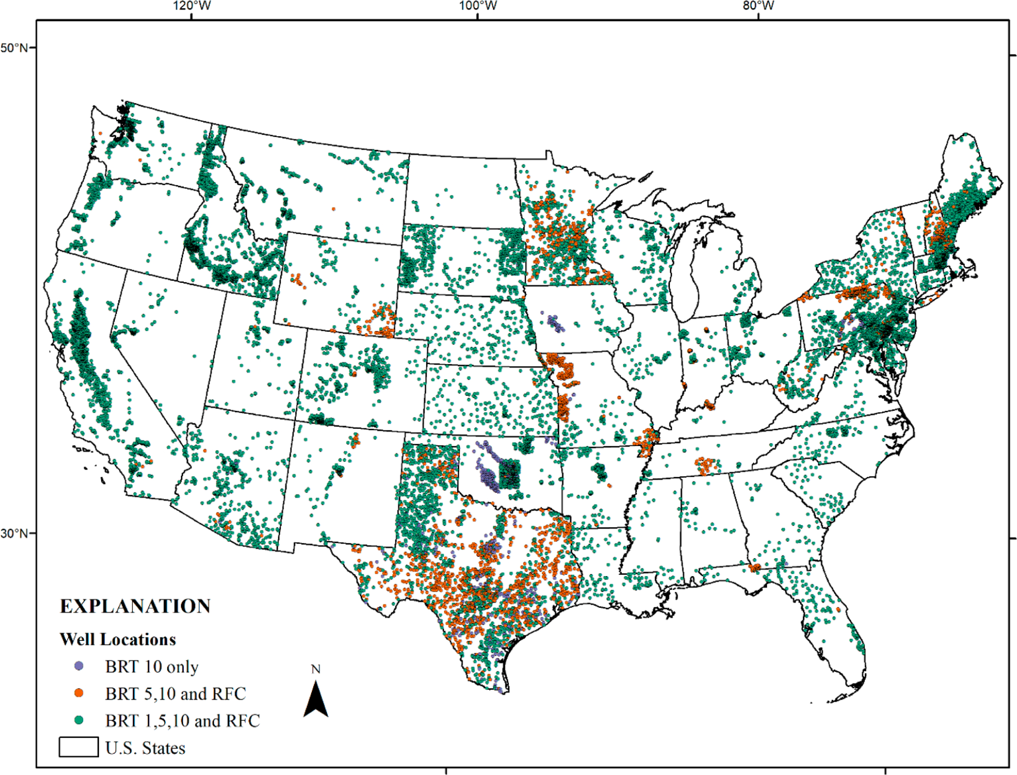
Locations of private wells and the model(s) in which each well is used.

BRT models were developed using a Bernoulli distribution of the model response term for each arsenic concentration threshold. Wells were coded with a 0 for concentrations less than or equal to the threshold and 1 for concentrations greater than the threshold. Model threshold concentrations were chosen to address existing public-supply drinking water guidelines (10 μg/L EPA MCL; 5 μg/L New Jersey and New Hampshire state MCL) and the common compliance monitoring method detection/quantitation limit (1 μg/L) (see for example ref 72) was chosen to address the EPA MCLG of zero.

The RFC model was developed to estimate the occurrence of arsenic in the concentration ranges of ≤5 μg/L, >5 to ≤10 μg/L, and >10 μg/L. Wells were coded based on the measured arsenic concentration category, with category 1 (C1) the lowest and category 3 (C3) the highest concentration. Preliminary RFC models, including one with 4 categories and a 1 μg/L boundary, were tested but not pursued due to poor model performance metrics. Due to differing arsenic concentration threshold values and varying reporting limits, not all 20,450 well data were suitable for use in every model. (Figure 1 and Table SI_2). Wells used in each model were subset into model training data sets (approximately 70% of available wells) and model testing data sets (approximately 30% of available wells). The proportion of wells above and below concentration thresholds for the BRT models and within the concentration categories for the RFC model were maintained between the training and testing data sets.

Model Variables.

Candidate variables considered for use in these models included geologic, geochemical, hydrologic, and climatic variables. General descriptions of the variables and their data sources are in Table SI_3. Some of the variables used in making the machine learning models are the same as those employed in the previous LR model,⁵⁸ including the base-flow index, percent of county land area containing tile drainage, soil geochemistry, and bedrock geology. The previous LR model used average annual groundwater recharge values estimated from the years 1951 to 1980⁷³ and average annual precipitation estimated from the years 1981 to 2000.⁷⁴ In the machine learning models developed in this study, average annual precipitation and groundwater recharge values are based on published estimates from the years 1981 to 2000 to optimize consistency between these two model variables.^75,76 Recently published variables included in the machine learning models that were not available for use in the LR model are the lateral position within a watershed for varying stream orders⁷⁷ and generalized rock type.⁷⁸

Due to correlations between variables from the same data set, not all available data were used. For example, soil geochemistry concentrations are available for various soil horizons however, at a given location the concentrations in individual horizons are highly correlated. Therefore, only the C soil horizon concentrations were selected to test in these models. Similarly, only the ecoregion level II valvalues⁸⁰d lateral position values for stream orders 2, 4, and 677 were considered in these models.

Values of all predictor variables were extracted for each well location using the ArcGIS software⁸¹ tools “spatial join” and “raster extract values to points”. All categorical variables, such as bedrock unit, were expanded so that the presence or absence of each type of bedrock unit became a variable. This resulted in a total of 249 variables that were tested to include in the models. No variables were missing at any of the well locations.

Model Development.

All models were developed using the R computing environment⁸² and tuned using the U.S. Geological Survey (USGS) Yeti Supercomputing cluster that has 3728 CPU cores (of which 100 were typically used) and approximately 105 TFlops performance.⁸³ BRT models were developed using the generalized boosted models⁸⁴ and caret⁸⁵ packages. A random forest classification (RFC) model was developed using the caret,⁸⁵ randomForest,⁸⁶ and rf Utilities⁸⁷ packages. BRT model tuning consisted of 720 combinations of the model hyper-parameters; number of trees (1000–5000, by 500), interaction depth (2–16, by 2), minimum observations in a node (8,10), and shrinkage rate (0.004–0.012, by 0.002). The RFC model tuning consisted of altering the number of variables randomly sampled as candidates at each split (mtry hyper-parameter) from 1 to 248 while the number of trees to grow (ntree) was maintained at 500. Descriptions of model hyper-parameters are given elsewhere.⁸⁸ All models were tuned using the training data set and 10-fold cross-validation to select the most accurate model using accuracy as the metric. To avoid selecting a model that was overfit to the model training data set, simpler models within one standard error of the most accurate models were identified (1SE models) and tested for selection as the final model. Simpler BRT models have a lower interaction depth, shrinkage rate, number of trees, and higher minimum observations in a node, while simpler RFC models have lower mtry values.⁸⁸

Metrics used to evaluate BRT model estimates compared to measured arsenic concentrations in private wells were total accuracy, sensitivity, specificity, kappa, and area under the receiver operating characteristic curve (ROC). Estimated probabilities greater than 0.5 were assigned above the model concentration threshold. Total accuracy is the ratio of correct model estimates to known well values divided by the total number of wells. In this study, models were developed to optimize total accuracy. Sensitivity is the ratio of correct estimates of the probability greater than 0.5 (or presence of arsenic above the threshold concentration) to the total number of wells with arsenic concentrations above the threshold concentration, or true positives. Specificity is the ratio of correct estimates of probabilities less than 0.5 to the total number of wells with arsenic concentrations less than or equal to the concentration threshold, or true negatives. Some studies shift the cut point from 0.5 to determine model specificity and sensitivity.^51,58,61 However, this does not change the underlying models, only the method for evaluating them. In this study we use the common cut point of 0.5 which allows for a consistent comparison of model performance across all models. The kappa statistic is a measure of agreement between model estimates and observations and includes expected accuracy under chance agreement. Kappa values range from -1 to 1 with a value of 1 indicating complete agreement between model estimates and observations, 0 representing what would be expected by chance, and negative values indicating agreement less than chance.⁸⁹ The area under the ROC considers using all possible cut-points (not only 0.5) to compare model estimates with observations. ROC values range from 0 to 1 with 1 indicating total agreement between model estimates and observations with 0.5 representing random guessing.⁹⁰ Metrics used to evaluate the RFC model include the kappa statistic and total accuracy, as defined above, in addition to producer’s accuracy and user’s accuracy. Producer’s accuracy is a measure of the total number of wells correctly classified by the model in a certain category divided by the total number of wells actually in that category.⁹¹ User’s accuracy is the number of wells the model correctly classifies in a category divided by the total number of wells the model classifies in that category.⁹¹ Model evaluation metrics were calculated for all wells throughout the CONUS and on a regional basis to evaluate potential spatial differences in model estimates. The CONUS was divided along state borders into 12 regions that correspond to regions defined by the USGS Ground Water Atlas of the United States.⁹²

The final models selected were the simplest models within 1SE of the most accurate model from tuning and had a reduced number of variables from the original 249 included for model development. The variables within each model were reduced by initially eliminating the variables that had no relative influence. Then the model was run sequentially, each time removing the least influential variable from the previous model run. The final number of variables selected minimized the loss in model accuracy and kappa from the model including all variables.

Model Estimate Maps.

Maps of model estimates for the CONUS were made using the final models. For each predictor variable in the final models, raster files with 1-km² grids were created in ArcMap and clipped to the same extent. BRT models can calculate estimates using predictor variables with missing data; however, RFC models cannot. Some model variable grids had cells with missing data at the CONUS scale; for the RFC model, missing data values were interpolated in ArcMap using the inverse-distance-weighted tool to make continuous estimate maps for the CONUS.⁸¹ The missing grid values were typically near coastlines and the border of the U.S. The model estimates were calculated from the raster files in R using the raster package⁹³ and output as geo-referenced tiff files. The model variable grid files and model output files are available to download in a separate USGS data release.⁷¹

Confidence intervals for the BRT model estimates were calculated using a bootstrapping technique explained elsewhere.⁹⁴

RESULTS AND DISCUSSION

Model Development.

Model tuning used all 249 variables to identify the most accurate model. Hyper-parameters of the final models were chosen from simpler models that were within one standard error of the most accurate model. Lastly, the number of variables within each model was reduced from the original 249. The final models contain between 41 and 65 variables. The final variables selected in the BRT models resulted in less than a 2% decrease in model performance metrics (accuracy, sensitivity, specificity) compared to the simpler 1SE model that included all variables. Reducing the number of variables selected in the RFC model decreased the total model accuracy by 3.85% but increased kappa by 9.83%. The hyper-parameters of the final models and the model prediction performance metrics are listed in Table 1.

Table 1.

Final Model Hyper-Parameters and Model Evaluation Metrics^a

	training data					testing data
model (interaction depth, shrinkage rate, number of trees, minimum observation in a node)	accuracy (%)	sensitivity (%)	specificity (%)	ROC	kappa	accuracy (%)	sensitivity (%)	specificity (%)	ROC	kappa
BRT1 (8, 0.010, 4500, 10)	86.4	84.3	88.2	0.941	0.727	77.2	74.1	80.0	0.853	0.542
BRT5 (10, 0.010, 5000, 8)	92.2	64.9	98.8	0.970	0.720	86.2	43.2	96.6	0.843	0.474
BRT10 (6, 0.010, 4500, 10)	94.1	49.9	99.4	0.952	0.617	91.2	33.9	98.2	0.850	0.413
RFC model predictions for training data
model	overall accuracy (%)	kappa	C1 user’s accuracy (%)	C2 user’s accuracy (%)	C3 user’s accuracy (%)	C1 producer’s accuracy (%)	C2 producer’s accuracy (%)	C3 producer’s accuracy (%)
mtry = 20	100	1.00	100	99.9	99.9	100	100	100
RFC model predictions for testing data
model	overall accuracy (%)	kappa	C1 user’s accuracy (%)	C2 user’s accuracy (%)	C3 user’s accuracy (%)	C1 producer’s accuracy (%)	C2 producer’s accuracy (%)	C3 producer’s accuracy (%)
mtry = 20	82.6	0.392	95.8	11.6	44.9	86.5	30.7	62.5

^aC1 = arsenic ≤5 μg/L, C2 = arsenic >5 to ≤10 μg/L, C3 = arsenic >10 μg/L.

Model Variables.

The definitions of the variables selected for the final models are listed in Table SI_4, and the variables included in each model and their relative influence are in Table SI_5. The 10 most influential variables in each model are shown in Figure 2 and many of the same variables are influential in each model. The most influential variable in all models is average annual precipitation from 1981 to 2010 (DMppt8110). Other highly influential variables in all four models are the arsenic, selenium, and phosphorus concentrations in the C soil horizon (as_c, se_c, p_c), lateral hydrologic position for sixth order streams (LP6), and average annual groundwater recharge from 1981 to 2010 (PRMS8110Re). Variables that are among the 10 most influential in 3 of the 4 models include base flow index (BFI) and the organic carbon and antimony concentrations in the C soil horizon (orgc_c, sb_c).

Figure 2.

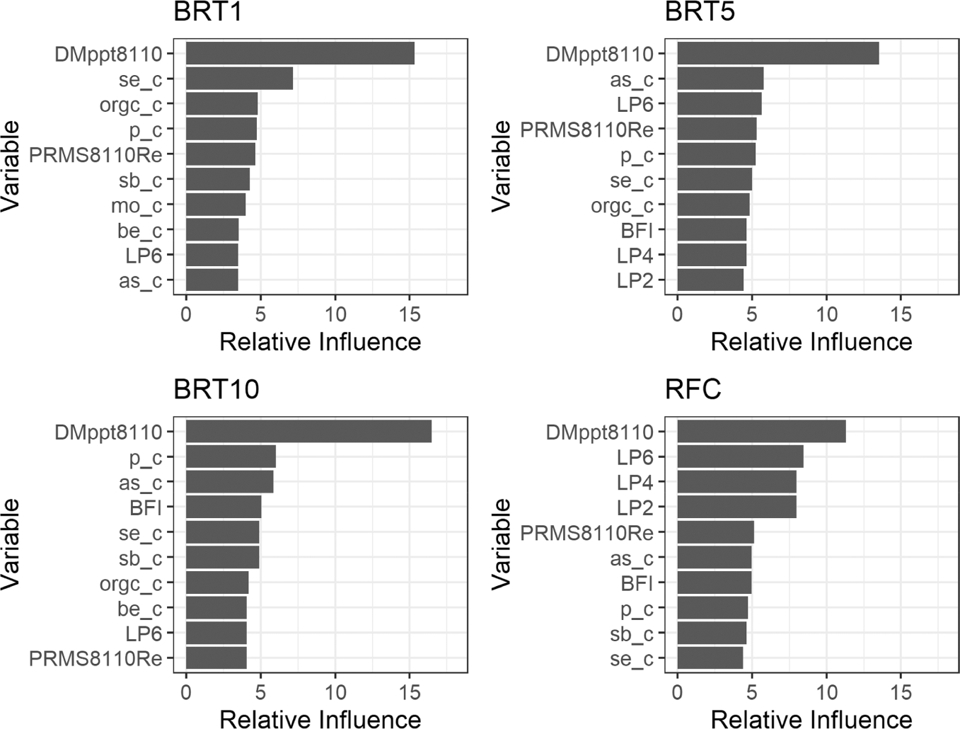
Ten most influential variables and their relative influence for each model. Variable definitions are in Table SI_4.

Partial dependence plots (PDPs) help qualitatively evaluate the relationships of the independent model variables to the model estimates. PDPs represent the partial dependence of the model estimate on the variable of interest considering the average effect of all other model variables.⁹⁵ The relationships depicted by PDPs may not be accurately represented in the presence of highly correlated predictor variables or in regions of the predictor variable space with sparse data.⁹⁶ The PDPs for average annual precipitation in the BRT and RFC models are shown in Figure 3 and PDPs for the 10 most influential variables in each model are shown in SI Figures 1–6. Rug plots (short vertical lines) along the x-axis on each plot indicate the deciles of the data available for each variable. The PDPs for the average annual precipitation variable in the BRT models indicate that the partial dependence of the probability of exceeding the arsenic concentration threshold generally decreases as the average annual precipitation increases (Figure 3). The PDPs for the RFC model vary by category within the model and the pattern in the PDP for C1 (As ≤ 5 μg/L) is opposite of those in C2 (As >5 to ≤10 μg/L) and C3 (>10 μg/L). However, they all indicate the same relationship because C1 is an estimate of the likelihood of being less than a concentration whereas C2 and C3 are predicting the likelihoods of being greater than or equal to certain arsenic concentrations. Interestingly, the PDPs for the RFC model have a pattern that shows a decrease in the partial dependence as average annual precipitation increases to approximately 1100 mm per year (mm/yr) followed by an increase in the partial dependence at precipitation values greater than 1100 mm/yr. This is a nonmonotonic pattern compared to the BRT models and seems to better reflect the spatial observations where elevated arsenic is present in both the dry desert southwest of the US and the more humid eastern portions of the country. In the previously developed LR model, average annual precipitation was also the most influential variable as determined by the absolute value of the standardized coeffcient (-0.706). The negative coeffcient indicates an inverse relationship between the average annual precipitation and the probability of arsenic >10 μg/L, similar to the pattern shown in the PDP for the BRT10 model.

Figure 3.

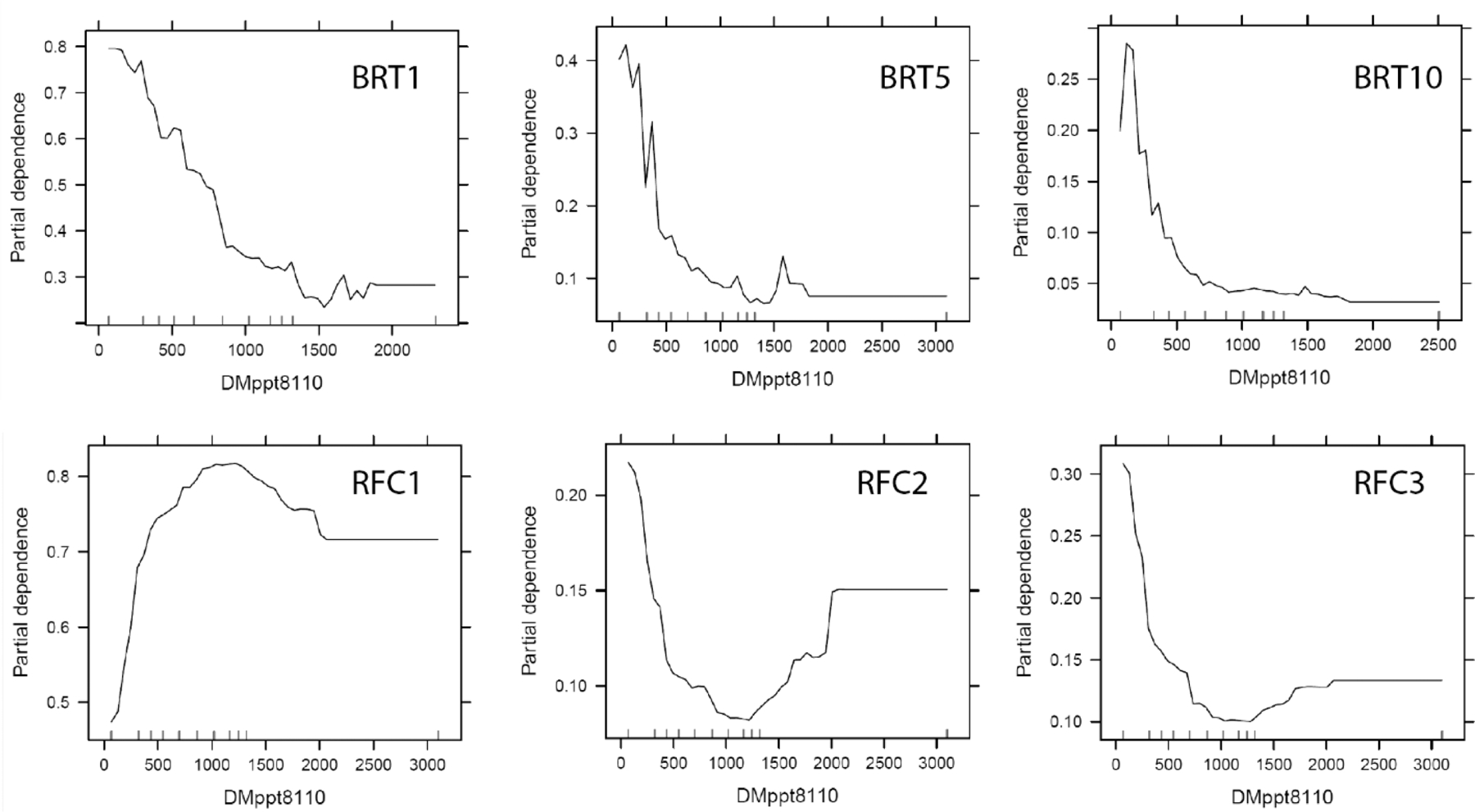
Partial dependence plots for average annual precipitation (DMppt8110) for the BRT models and each classification within the RFC model. Note the different scales on the y-axes.

Several soil geochemistry variables are influential in the machine learning models, including arsenic, selenium, phosphorus, organic carbon, and antimony concentrations in the C soil horizon. The arsenic concentrations in the C soil horizon have a nonmonotonic relationship with the partial dependence of arsenic concentrations in private wells being above the various model concentration thresholds. The PDPs indicate an inverse relationship at low soil arsenic concentrations and a direct relationship at higher concentrations (See Figures SI_1–6). These results are consistent with previous studies that indicate the presence of arsenic in host aquifer materials alone is not necessarily a good indication of arsenic concentrations in the corresponding groundwater; the dissolution of arsenic from the aquifer host material is also dependent on the redox and pH conditions of the aquifer.^7,97 The general pattern of organic carbon concentrations in the C soil horizon in the PDPs shows a direct relationship with the probability of arsenic in private well water exceeding the arsenic concentration threshold for the models. This pattern is also consistent with previous studies that show the presence of organic carbon facilitates reductive dissolution of arsenic from aquifer sediments coated with iron oxyhydroxide minerals.^7,98,99 The PDPs for selenium and phosphorus are more di?cult to interpret because they do not exhibit consistent patterns.

Model Performance Metrics.

The performance metrics for the final models are in Table 1. The models were developed to optimize overall prediction accuracy, which ranges from 77 to 91% for testing data. The overall model accuracy for the BRT models increases with an increase in arsenic concentration threshold. This is driven by the increase in model specificity or correct estimates of locations below the arsenic concentration thresholds. The models do very well estimating where arsenic is not likely to occur as quantified by the BRT model specificities, which range from 80 to 98% for testing data. For the application of our models to similarly scaled data on human health outcomes, the identification of areas where arsenic is not likely to be elevated is just as important as identification of areas where arsenic is likely to be elevated. The model specificities decrease with a decrease in the arsenic concentration threshold. BRT model sensitivities are lower and range from 34 to 74% for testing data and decrease with higher arsenic concentration thresholds.

The patterns in model performance metrics are largely driven by the underlying arsenic concentration data used to develop the models. The lower model sensitivities as compared to the specificities are caused by the infrequent occurrence of high arsenic concentrations in our data set and the high well-to-well variability of arsenic that can occur in wells within proximity of each other.¹⁰⁰ It is inherently more diffcult for the models to correctly predict events in the data that do not occur frequently. The ability of the BRT10 model to accurately estimate locations where wells exceed 10 μg/L is relatively low (33.9%) because only 11% of the wells in our data set have concentrations above 10 μg/L. The BRT1 model is better at predicting arsenic concentrations above 1 μg/L because approximately 48% of the private wells in our data set have arsenic concentrations above 1 μg/L (Table SI_2). As indicated by the decreased sensitivity with higher arsenic concentration thresholds, model accuracy depends on the amount of data and the percentage of events in those data. The same pattern exists in the performance metrics for the RFC model where C2, the category with the least number of occurrences in the data set (8.4%), has the lowest user’s and producer’s accuracy. In addition to the underlying distribution of data used to develop our models, the high variability of arsenic concentrations in wells within proximity of each other may contribute to the low sensitivity values observed in some of our models. We caution against diminishing the usefulness of these models due to the low sensitivity values and instead emphasize the high overall accuracy (77–91%) and specificity (80–98%) of the models. The identification of areas where arsenic is not likely to occur in domestic wells is important information.

While the development of regional scale models would not have achieved our goal of developing nationally consistent estimates, we did evaluate model performance at regional scales and results are in Tables SI_6 to SI_16. It is difficult to make meaningful conclusions based on the regional results because of the imbalance of data available across regions and the infrequent occurrence of arsenic above the concentration thresholds for the BRT5 and BRT10 models. Some regions contain relatively small numbers of wells in the testing data set (~100 wells) and no to few wells with arsenic concentrations above the model thresholds. Regional model evaluation metrics for the BRT1 model, which contains a greater occurrence of wells above the arsenic concentration threshold compared to the BRT5 and BRT10 models, do indicate regional variations in model accuracy. Some regions have sensitivity values greater than specificity indicating the BRT1 model is better at estimating where wells exceed the 1 μg/L arsenic concentration threshold in those regions. Several regional scale statistical models have been developed to predict arsenic occurrence in groundwater and incorporate spatially detailed and relevant predictor variables available for the areas of interest.^51,52,65,69 For example, a model developed for the Central Valley aquifer of California includes variables that are outputs from numerical models developed specifically for that aquifer.⁵¹ In this study we only include predictor variables available across the CONUS resulting in a nationally coherent model.

The model performance metrics from the BRT10 model can be compared to the previous LR model that estimated the probability of arsenic exceeding 10 μg/L.⁵⁸ The overall accuracy and specificity of the two models to testing data are similar; LR accuracy is 90.1% and BRT10 accuracy is 91.2%, and LR specificity is 99% and BRT10 specificity is 98.2%. The two models differ in their sensitivity, or ability to correctly predict where there is a high probability of arsenic being greater than 10 μg/L. The sensitivity of the LR model to testing data is 13.9% and the sensitivity of the BRT10 model is 33.9%, suggesting the BRT10 model is better at predicting areas with high levels of arsenic in private wells. The BRT10 model is an incremental improvement of the previously developed LR model. This result is similar to findings from a study that developed and compared BRT and LR models to estimate arsenic in domestic and public supply wells located in the Central Valley of California.⁵¹

Model Estimate Maps.

The final models were applied to 1-km² grids to produce model estimate maps for the CONUS. Results for the BRT models are shown in Figure 4a–c and indicate the probability of exceeding the arsenic concentration threshold for each model. RFC model estimates of the probability of being in C1, C2, and C3 are shown in Figures 4d–f, respectively, and the most likely classification from the RFC model is shown in Figure 4g.

Figure 4.

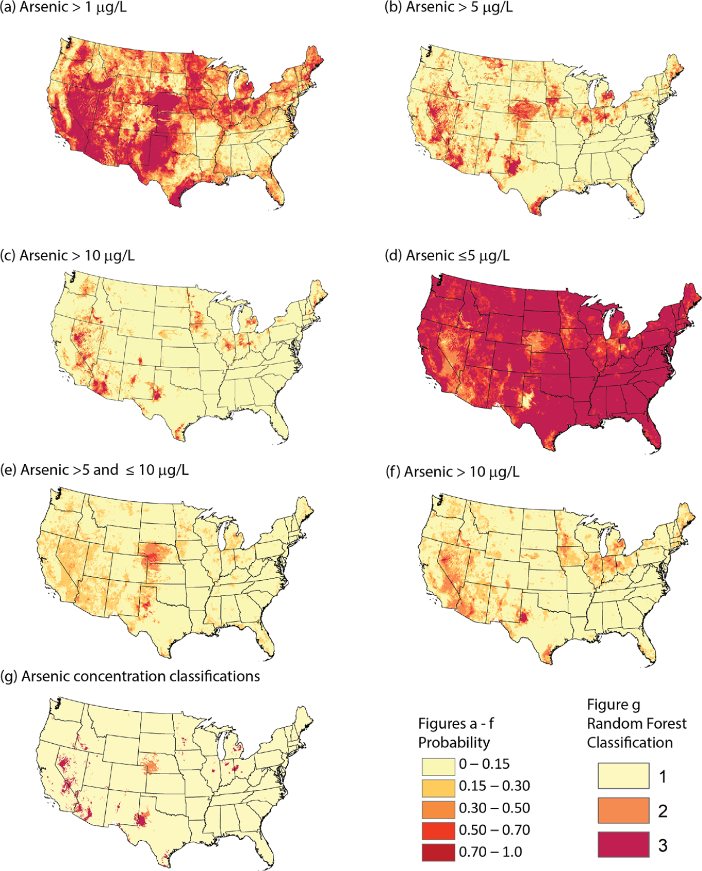
Probability of arsenic (a) greater than 1 μg/L from BRT1 model, (b) greater than 5 μg/L from BRT5 model, (c) greater than 10 μg/L from BRT10 model, (d) less than or equal to 5 μg/L from RFC model, (e) greater than 5 μg/L and less than or equal to 10 μg/L from RFC model, and (f) greater than 10 μg/L from RFC model. Panel (g) estimated arsenic concentration classification from RFC model.

Direct comparisons between the various BRT models are not recommended because the models were developed independently. However, the results across models are generally consistent with each other at the national scale (Figures 4a–c). The RFC model was developed to facilitate comparisons across the arsenic concentration categories, the probabilities of occurring in each category at a given location are consistent with each other because they are calculated from the same model. The RFC model also provides an arsenic concentration category estimate for a given location (Figure 4g), which can be used to examine dose-response in health studies, as opposed to the BRT model estimates that provide a single probability of exceeding an arsenic concentration threshold. Although the BRT10 and RFC models are not directly comparable, they do exhibit similar patterns. For example, both models have probabilities >70% for arsenic concentrations >10 μg/L along eastern California, southeast New Mexico, and throughout the midwestern states as shown in Figure 4c,f. Comparison of map estimates from this study to the previous study using an LR model⁵⁸ also show similar patterns across the CONUS with >50% probability of arsenic >10 μg/L in areas of the Southwest, Texas, the Midwest, and New England. Areas of >50% probability are more sharply defined in the BRT10 map estimates compared to the LR map and this reflects the difference in the ability of the BRT model to correctly predict areas of high arsenic (increased model sensitivity). As indicated by the model performance metrics, these models do well at estimating locations where the probability of exceeding the concentration threshold for arsenic is low. The model estimate maps are an important tool for estimating arsenic occurrence, or lack of occurrence, especially in areas that do not have actual well water samples. In the absence of arsenic sampling data, these models provide a best estimate of arsenic occurrence throughout the CONUS.

Confidence intervals for the BRT model estimates were calculated and are shown in Figure SI_7. The confidence intervals account for uncertainties in the model estimates and do not consider uncertainties associated with the variables used to make the models.

Limitations.

Our model estimates were produced for 1-km² grids. However, we caution against interpreting these results at the 1-km² scale because these models and maps were developed using predictor variable data sets available at the CONUS scale. Multistate regional and/or smaller geographic area scale models using regionally available and relevant predictor variable data may provide more representative results at those spatial scales. Model estimates in this study are made for large areas that do not have arsenic data from private wells such as northern Vermont, eastern Kentucky, eastern New Mexico, and southern Nevada (Figure 1). The accuracy of our model estimates in these sparsely sampled areas cannot be assessed without additional sampling. Additionally, improved model prediction sensitivity may result from additional sampling, especially in areas with elevated arsenic concentrations.

Our model estimates for arsenic are static in time. However, they are based on water samples collected from 1970 to 2013, and the models include variables that change temporally such as average annual precipitation and groundwater recharge. Thirty-year climate averages were used for these variables in our models. There is growing evidence of seasonal and climate-related changes in arsenic concentrations in groundwater.^101–103 Temporal changes are not considered in this study and our estimates represent climate averages. The long period over which the arsenic samples were collected contributes to potential uncertainty due to possible temporal variation.

These models were developed using data from private wells, which approximately 15% of the population use for drinking water supply.^40–42 The model estimates should be used to estimate exposure to arsenic from private wells and may not accurately estimate exposure from public drinking water supplies. Public water supplies include water sources from both surface water and groundwater, are regulated by the EPA, are tested regularly, and typically have treatment systems to comply with the MCL for arsenic. Therefore, our model estimates may not correctly represent the arsenic exposure from drinking water in urban and densely populated areas that rely on public drinking water systems.

Continual refinement of models to better represent geogenic contaminant concentrations, such as arsenic, where the well-to-well concentration variability is several orders of magnitude is an area of ongoing research. Development and inclusion of relevant predictor variables that represent geochemical mechanisms responsible for arsenic mobilization in groundwater such as pH and redox conditions will likely lead to better predictive performance of arsenic models. Regional scale models have recently been developed to characterize and predict these important covariates and provide opportunities to improve statistical models of geogenic groundwater contamination at all scales.^104–106 The development of these characterizations, especially as they change with well depth, will presumably expand the capabilities of modeling the occurrence of arsenic in groundwater by improving model accuracy and reducing uncertainty.

Use of the Model Estimate Maps in Human Health Studies.

The model estimates provide an important, feasible, and complementary perspective to the existing arsenic epidemiology literature by offering national inferences for the U.S. and serve as a foundation for future investigations. For example, epidemiological modeling efforts might potentially identify “hot spots” (e.g., counties where there may be an unusually strong relationship between arsenic and disease frequency) that could be appropriate for more targeted community-level investigations.

Linking human-health outcomes to environmental exposure can be challenging when the data are available on different geographic scales or no exposure data are available. However, methods are increasingly being developed to make these linkages more achievable.^107,108 The previously developed LR model was used as a covariate in studies of national scale human health data.^109,110 The machine learning models developed here are an improvement upon the previous model and will provide additional information for future environmental epidemiology studies. Until now, spatially continuous geographic data on arsenic occurrence at varying concentrations in private-supply drinking water has been lacking within the U.S. Our arsenic models provide a new and coherent resource to evaluate associations of private well arsenic occurrence at various concentrations with human health outcomes at the CONUS scale.

Another difficulty in conducting environmental epidemiology studies is exposure assessment. It is often challenging to identify a population with a range of exposures that is sufficiently broad to assess dose-response, where the response is a clinical biomarker value or health outcome. Our models provide a robust tool to estimate arsenic occurrence over a range of concentrations and potential exposure from private wells for a large population. These models indicate geographic areas where people are unlikely to be exposed and where they are likely to be exposed to arsenic from private wells. This allows researchers to target areas with potentially high and low exposure levels thereby increasing the power of future studies to detect associations with relevant health outcomes. Our models are well suited for comparison and evaluation of potential relations to similarly scaled human health data.

REFERENCES

- (1).Naujokas MF; Anderson B; Ahsan H; Aposhian HV; Graziano JH; Thompson C; Suk WA The broad scope of health effects from chronic arsenic exposure: update on a worldwide public health problem. Environ. Health Perspect. 2013, 121 (3), 295–302. [DOI] [PMC free article] [PubMed] [Google Scholar]
- (2).WHO, 2011, Guidelines for Drinking-water Quality, 4th edition; https://www.who.int/water_sanitation_health/water-quality/guidelines/chemicals/arsenic-fs-new.pdf.
- (3).Argos M; Ahsan H; Graziano JH Arsenic and human health: epidemiologic progress and public health implications. Rev. Environ. Health 2012, 27 (4), 191–195. [DOI] [PMC free article] [PubMed] [Google Scholar]
- (4).Mantha M; Yeary E; Trent J; Creed PA; Kubachka K; Hanley T; Shockey N; Heitkemper D; Caruso J; Xue J; Rice G; Wymer L; Creed JT Estimating Inorganic Arsenic Exposure from U.S. Rice and Total Water Intakes. Environ. Health Perspect. 2017, 125 (5), 057005. [DOI] [PMC free article] [PubMed] [Google Scholar]
- (5).U.S. Environmental Protection Agency. National Primary Drinking Water Regulations. https://www.epa.gov/ground-waterand-drinking-water/national-primary-drinking-water-regulations (1/11/18).
- (6).U.S. Environmental Protection Agency. How EPA Regulates Drinking Water Contaminants. https://www.epa.gov/dwregdev/howepa-regulates-drinking-water-contaminants (7/26/18).
- (7).Smedley PL; Kinniburgh DG A review of the source, behaviour and distribution of arsenic in natural waters. Appl. Geochem. 2002, 17, 517–568. [Google Scholar]
- (8).Kuo C-C; Moon KA; Wang S-L; Silbergeld E; Navas-Acien A The Association of Arsenic Metabolism with Cancer, Cardiovascular Disease, and Diabetes: A Systematic Review of the Epidemiological Evidence. Environ. Health Perspect. 2017, 125 (8), 087001. [DOI] [PMC free article] [PubMed] [Google Scholar]
- (9).Argos M; Parvez F; Rahman M; Rakibuz-Zaman M; Ahmed A; Hore SK; Islam T; Chen Y; Pierce BL; Slavkovich V; Olopade C; Yunus M; Baron JA; Graziano JH; Ahsan H Arsenic and lung disease mortality in Bangladeshi adults. Epidemiology 2014, 25 (4), 536–543. [DOI] [PMC free article] [PubMed] [Google Scholar]
- (10).Sanchez TR; Powers M; Perzanowski M; George CM; Graziano JH; Navas-Acien A A Meta-analysis of Arsenic Exposure and Lung Function: Is There Evidence of Restrictive or Obstructive Lung Disease? Curr. Environ. Health Rep 2018, 5 (2), 244–254. [DOI] [PMC free article] [PubMed] [Google Scholar]
- (11).Jiang J; Liu M; Parvez F; Wang B; Wu F; Eunus M; Bangalore S; Newman JD; Ahmed A; Islam T; Rakibuz-Zaman M; Hasan R; Sarwar G; Levy D; Slavkovich V; Argos M; Bryan MS; Farzan SF; Hayes RB; Graziano JH; Ahsan H; Chen Y Association between Arsenic Exposure from Drinking Water and Longitudinal Change in Blood Pressure among HEALS Cohort Participants. Environ. Health Perspect. 2015, 123 (8), 806–812. [DOI] [PMC free article] [PubMed] [Google Scholar]
- (12).Scannell Bryan M; Sofer T; Mossavar-Rahmani Y; Thyagarajan B; Zeng D; Daviglus ML; Argos M Mendelian randomization of inorganic arsenic metabolism as a risk factor for hypertension- and diabetes-related traits among adults in the Hispanic Community Health Study/Study of Latinos (HCHS/SOL) cohort. International Journal of Epidemiology 2019, 48 (3), 876–886. [DOI] [PMC free article] [PubMed] [Google Scholar]
- (13).Shen H; Xu W; Zhang J; Chen M; Martin FL; Xia Y; Liu L; Dong S; Zhu Y-G Urinary Metabolic Biomarkers Link Oxidative Stress Indicators Associated with General Arsenic Exposure to Male Infertility In a Han Chinese Population. Environ. Sci. Technol. 2013, 47 (15), 8843–8851. [DOI] [PubMed] [Google Scholar]
- (14).Cohen SM; Chowdhury A; Arnold LL Inorganic arsenic: A non-genotoxic carcinogen. J. Environ. Sci. 2016, 49,28–37. [DOI] [PubMed] [Google Scholar]
- (15).Lauer FT; Parvez F; Factor-Litvak P; Liu X; Santella RM; Islam T; Eunus M; Alam N; Hasan AKMR; Rahman M; Ahsan H; Graziano J; Burchiel SW Changes in human peripheral blood mononuclear cell (HPBMC) populations and T-cell subsets associated with arsenic and polycyclic aromatic hydrocarbon exposures in a Bangladesh cohort. PLoS One 2019, 14 (7), No. e0220451. [DOI] [PMC free article] [PubMed] [Google Scholar]
- (16).Wasserman GA; Liu X; Parvez F; Ahsan H; Factor-Litvak P; van Geen A; Slavkovich V; Lolacono NJ; Cheng Z; Hussain I; Momotaj H; Graziano JH Water Arsenic Exposure and Children’s Intellectual Function in Araihazar, Bangladesh. Environ. Health Perspect. 2004, 112 (13), 1329–1333. [DOI] [PMC free article] [PubMed] [Google Scholar]
- (17).Kuo C-C; Howard BV; Umans JG; Gribble MO; Best LG; Francesconi KA; Goessler W; Lee E; Guallar E; Navas-Acien A Arsenic Exposure, Arsenic Metabolism, and Incident Diabetes in the Strong Heart Study. Diabetes Care 2015, 38 (4), 620–627. [DOI] [PMC free article] [PubMed] [Google Scholar]
- (18).Argos M; Kalra T; Pierce BL; Chen Y; Parvez F; Islam T; Ahmed A; Hasan R; Hasan K; Sarwar G; Levy D; Slavkovich V; Graziano JH; Rathouz PJ; Ahsan H A Prospective Study of Arsenic Exposure From Drinking Water and Incidence of Skin Lesions in Bangladesh. Am. J. Epidemiol. 2011, 174 (2), 185–194. [DOI] [PMC free article] [PubMed] [Google Scholar]
- (19).Karagas MR; Gossai A; Pierce B; Ahsan H Drinking Water Arsenic Contamination, Skin Lesions, and Malignancies: A Systematic Review of the Global Evidence. Curr. Environ. Health Rep 2015, 2 (1), 52–68. [DOI] [PMC free article] [PubMed] [Google Scholar]
- (20).Liaw J; Marshall G; Yuan Y; Ferreccio C; Steinmaus C; Smith AH Increased Childhood Liver Cancer Mortality and Arsenic in Drinking Water in Northern Chile. Cancer Epidemiol., Biomarkers Prev. 2008, 17 (8), 1982–1987. [DOI] [PMC free article] [PubMed] [Google Scholar]
- (21).Liu J; Waalkes MP Liver is a Target of Arsenic Carcinogenesis. Toxicol. Sci. 2008, 105 (1), 24–32. [DOI] [PMC free article] [PubMed] [Google Scholar]
- (22).Yuan Y; Marshall G; Ferreccio C; Steinmaus C; Liaw J; Bates M; Smith AH Kidney cancer mortality: fifty-year latency patterns related to arsenic exposure. Epidemiology 2010, 21 (1), 103–108. [DOI] [PubMed] [Google Scholar]
- (23).Mendez WM Jr.; Eftim S; Cohen J; Warren I; Cowden J; Lee JS; Sams R Relationships between arsenic concentrations in drinking water and lung and bladder cancer incidence in U.S. counties. J. Exposure Sci. Environ. Epidemiol. 2017, 27 (3), 235–243. [DOI] [PubMed] [Google Scholar]
- (24).Baris D; Waddell R; Beane Freeman LE; Schwenn M; Colt JS; Ayotte JD; Ward MH; Nuckols J; Schned A; Jackson B; Clerkin C; Rothman N; Moore LE; Taylor A; Robinson G; Hosain GM; Armenti KR; McCoy R; Samanic C; Hoover RN; Fraumeni JF Jr.; Johnson A; Karagas MR; Silverman DT Elevated Bladder Cancer in Northern New England: The Role of Drinking Water and Arsenic. J. Natl. Cancer Inst 2016, 108 (9), No. djw099. [DOI] [PMC free article] [PubMed] [Google Scholar]
- (25).Carlin DJ; Naujokas MF; Bradham KD; Cowden J; Heacock M; Henry HF; Lee JS; Thomas DJ; Thompson C; Tokar EJ; Waalkes MP; Birnbaum LS; Suk WA Arsenic and Environmental Health: State of the Science and Future Research Opportunities. Environ. Health Perspect. 2016, 124 (7), 890–899. [DOI] [PMC free article] [PubMed] [Google Scholar]
- (26).Chen Y; Ahsan H Cancer Burden From Arsenic in Drinking Water in Bangladesh. Am. J. Public Health 2004, 94 (5), 741–744. [DOI] [PMC free article] [PubMed] [Google Scholar]
- (27).Hughes MF Arsenic toxicity and potential mechanisms of action. Toxicol. Lett. 2002, 133 (1), 1–16. [DOI] [PubMed] [Google Scholar]
- (28).Rahman A; Vahter M; Ekström E-C; Rahman M; Golam Mustafa AHM; Wahed MA; Yunus M; Persson L-Å Association of Arsenic Exposure during Pregnancy with Fetal Loss and Infant Death: A Cohort Study in Bangladesh. Am. J. Epidemiol. 2007, 165 (12), 1389–1396. [DOI] [PubMed] [Google Scholar]
- (29).Shih Y-H; Islam T; Hore SK; Sarwar G; Shahriar MH; Yunus M; Graziano JH; Harjes J; Baron JA; Parvez F; Ahsan H; Argos M Associations between prenatal arsenic exposure with adverse pregnancy outcome and child mortality. Environ. Res. 2017, 158, 456–461. [DOI] [PMC free article] [PubMed] [Google Scholar]
- (30).Ayotte JD; Baris D; Cantor KP; Colt J; Robinson GR Jr.; Lubin JH; Karagas M; Hoover RN; Fraumeni JF Jr.; Silverman DT Bladder cancer mortality and private well use in New England: an ecological study. J. Epidemiol Community Health 2006, 60 (2), 168–72. [DOI] [PMC free article] [PubMed] [Google Scholar]
- (31).U.S. Environmental Protection Agency 40 C.F.R. § 131: Water Quality Standards 40 C.F.R. § 131, 2017, https://www.ecfr.gov/cgi-bin/text-idx?SID=454a7b51118b27f20cef29?071c1440&node=40:22.0.1.1.18&rgn=div5.
- (32).New Hampshire State House, HB261, Requiring the commissioner of the department of environmental services to revise rules relative to arsenic contamination in drinking water, https://legiscan.com/NH/text/HB261/2019.
- (33).Code NJA Safe Drinking Water Act Rules 7:10, 2018, https://www.nj.gov/dep/rules/rules/njac7_10.pdf.
- (34).Ahmad A; Bhattacharya P Arsenic in Drinking Water: Is 10 μg/L a Safe Limit? Current Pollution Reports 2019, 5 (1), 1–3. [Google Scholar]
- (35).Ahmad A; van der Wens P; Baken K; de Waal L; Bhattacharya P; Stuyfzand P Arsenic reduction to < 1 μg/L in Dutch drinking water. Environ. Int. 2020, 134, 105253. [DOI] [PubMed] [Google Scholar]
- (36).Gong G; O’Bryant SE Low-level arsenic exposure, AS3MT gene polymorphism and cardiovascular diseases in rural Texas counties. Environ. Res. 2012, 113,52–57. [DOI] [PubMed] [Google Scholar]
- (37).Moon KA; Guallar E; Umans JG; Devereux RB; Best LG; Francesconi KA; Goessler W; Pollak J; Silbergeld EK; Howard BV; Navas-Acien A Association Between Exposure to Low to Moderate Arsenic Levels and Incident Cardiovascular Disease: A Prospective Cohort Study. Ann. Int. Med. 2013, 159 (10), 649–659. [DOI] [PMC free article] [PubMed] [Google Scholar]
- (38).Roh T; Lynch CF; Weyer P; Wang K; Kelly KM; Ludewig G Low-level arsenic exposure from drinking water is associated with prostate cancer in Iowa. Environ. Res. 2017, 159, 338–343. [DOI] [PMC free article] [PubMed] [Google Scholar]
- (39).Tsuji JS; Garry MR; Perez V; Chang ET Low-level arsenic exposure and developmental neurotoxicity in children: A systematic review and risk assessment. Toxicology 2015, 337,91–107. [DOI] [PubMed] [Google Scholar]
- (40).Johnson TD; Belitz K; Lombard MA Estimating domestic well locations and populations served in the contiguous U.S. for years 2000 and 2010. Sci. Total Environ. 2019, 687, 1261–1273. [DOI] [PubMed] [Google Scholar]
- (41).Maupin MA, 2018, Summary of estimated water use in the United States in 2015; U. S. Geological Survey Fact Sheet 2018–3035, DOI: 10.3133/fs20183035. [DOI] [Google Scholar]
- (42).Dieter CA; Maupin MA; Caldwell RR; Harris MA; Ivahnenko TI; Lovelace JK; Barber NL; Linsey KS Estimated use of water in the United States in 2015. U.S. Geological Survey Circular 1441, 2018, 65. [Google Scholar]
- (43).U.S. Environmental Protection Agency. Private drinking water wells. https://www.epa.gov/privatewells (1/10/18).
- (44).Swistock BR; Clemens S Water quality and management of private drinking water wells in Pennsylvania. Journal of environmental health 2013, 75 (6), 60. [PubMed] [Google Scholar]
- (45).Focazio MJ; Tipton D; Dunkle Shapiro S; Geiger LH The chemical quality of self-supplied domestic well water in the United States. Groundwater Monit. Rem. 2006, 26 (3), 92–104. [Google Scholar]
- (46).Seltenrich N Unwell: The Public Health Implications of Unregulated Drinking Water. Environ. Health Perspect. 2017, 125 (11), 114001–114001. [DOI] [PMC free article] [PubMed] [Google Scholar]
- (47).MacDonald Gibson J; Pieper KJ Strategies to Improve Private-Well Water Quality: A North Carolina Perspective. Environ. Health Perspect. 2017, 125 (7), 076001–076001. [DOI] [PMC free article] [PubMed] [Google Scholar]
- (48).DeSimone LA Quality of Water from Domestic Wells in Principal Aquifers of the United States, 1991–2004. U. S. Geological Survey Scientific Investigations Report 2008–5227 2009, 139. [Google Scholar]
- (49).DeSimone LA; McMahon PB; Rosen MR The quality of our Nation’s waters: Water quality in principal aquifers of the United States, 1991–2010. U.S. Geological Survey Circular 1360, 2015, 151. [Google Scholar]
- (50).Ayotte JD; Cahillane M; Hayes L; Robinson KW, 2012, Estimated Probability of Arsenic in Groundwater from Bedrock Aquifers in New Hampshire, 2011; U.S. Geological Survey Scientific Investigations Report 2012–5156, http://pubs.usgs.gov/sir/2012/5156/. [Google Scholar]
- (51).Ayotte JD; Nolan BT; Gronberg JA Predicting Arsenic in Drinking Water Wells of the Central Valley, California. Environ. Sci. Technol. 2016, 50 (14), 7555–63. [DOI] [PubMed] [Google Scholar]
- (52).Ayotte JD; Nolan BT; Nuckols JR; Cantor KP; Robinson GR; Baris D; Hayes L; Karagas M; Bress W; Silverman DT; Lubin JH Modeling the Probability of Arsenic in Groundwater in New England as a Tool for Exposure Assessment. Environ. Sci. Technol. 2006, 40 (11), 3578–3585. [DOI] [PubMed] [Google Scholar]
- (53).Gross EL; Low DJ Arsenic concentrations, related environmental factors, and the predicted probability of elevated arsenic in groundwater in Pennsylvania. U.S. Geological Survey Scientific Investigations Report 2012–5257 2013, 46.
- (54).Kim D; Miranda ML; Tootoo J; Bradley P; Gelfand AE Spatial Modeling for Groundwater Arsenic Levels in North Carolina. Environ. Sci. Technol. 2011, 45 (11), 4824–4831. [DOI] [PMC free article] [PubMed] [Google Scholar]
- (55).Twarakavi NKC; Kaluarachchi JJ Aquifer vulnerability assessment to heavy metals using ordinal logistic regression. Groundwater 2005, 43 (2), 200–214. [DOI] [PubMed] [Google Scholar]
- (56).Winkel LHE; Trang PTK; Lan VM; Stengel C; Amini M; Ha NT; Viet PH; Berg M Arsenic pollution of groundwater in Vietnam exacerbated by deep aquifer exploitation for more than a century. Proc. Natl. Acad. Sci. U. S. A. 2011, 108 (4), 1246–51. [DOI] [PMC free article] [PubMed] [Google Scholar]
- (57).Winkel L; Berg M; Amini M; Hug SJ; Annette Johnson C Predicting groundwater arsenic contamination in Southeast Asia from surface parameters. Nat. Geosci. 2008, 1 (8), 536–542. [Google Scholar]
- (58).Ayotte JD; Medalie L; Qi SL; Backer LC; Nolan BT Estimating the High-Arsenic Domestic-Well Population in the Conterminous United States. Environ. Sci. Technol. 2017, 51 (21), 12443–12454. [DOI] [PMC free article] [PubMed] [Google Scholar]
- (59).Rodríguez-Lado L; Sun G; Berg M; Zhang Q; Xue H; Zheng Q; Johnson CA Groundwater Arsenic Contamination Throughout China. Science 2013, 341 (6148), 866. [DOI] [PubMed] [Google Scholar]
- (60).Bretzler A; Lalanne F; Nikiema J; Podgorski J; Pfenninger N; Berg M; Schirmer M Groundwater arsenic contamination in Burkina Faso, West Africa: Predicting and verifying regions at risk. Sci. Total Environ. 2017, 584–585, 958–970. [DOI] [PubMed] [Google Scholar]
- (61).Podgorski JE; Eqani SAMAS; Khanam T; Ullah R; Shen H; Berg M Extensive arsenic contamination in high-pH unconfined aquifers in the Indus Valley. Science Advances 2017, 3 (8), No. e1700935. [DOI] [PMC free article] [PubMed] [Google Scholar]
- (62).Amini M; Abbaspour KC; Berg M; Winkel L; Hug SJ; Hoehn E; Yang H; Johnson CA Statistical Modeling of Global Geogenic Arsenic Contamination in Groundwater. Environ. Sci. Technol. 2008, 42 (10), 3669–3675. [DOI] [PubMed] [Google Scholar]
- (63).Hosmer DW; Lemeshow S Applied Logistic Regression, 2nd ed; John Wiley & Sons, Inc.: New York, 2000. [Google Scholar]
- (64).Breiman L Statistical Modeling: The Two Cultures. Statistical Science 2001, 16 (3), 199–231. [Google Scholar]
- (65).Anning DW; Paul AP; McKinney TS; Huntington JM; Bexfield LM; Thiros SA Predicted nitrate concentrations in basin-fill aquifers of the Southwestern United States. U.S. Geological Survey Scientific Investigations Report 2012–5065 2012, 78.
- (66).Smith R; Knight R; Fendorf S Overpumping leads to California groundwater arsenic threat. Nat. Commun. 2018, 9 (1), 2089. [DOI] [PMC free article] [PubMed] [Google Scholar]
- (67).Tesoriero AJ; Gronberg JA; Juckem PF; Miller MP; Austin BP Predicting redox-sensitive contaminant concentrations in groundwater using random forest classification. Water Resour. Res. 2017, 53 (8), 7316–7331. [Google Scholar]
- (68).Bindal S; Singh CK Predicting groundwater arsenic contamination: Regions at risk in highest populated state of India. Water Res. 2019, 159,65–76. [DOI] [PubMed] [Google Scholar]
- (69).Erickson ML; Elliott SM; Christenson CA; Krall AL, Predicting geogenic arsenic in drinking water wells in glacial aquifers, north-central USA: accounting for depth-dependent features. Water Resour. Res. 2018, DOI: 10.1029/2018WR023106. [DOI] [Google Scholar]
- (70).Frederick L; VanDerslice J; Taddie M; Malecki K; Gregg J; Faust N; Johnson WP Contrasting regional and national mechanisms for predicting elevated arsenic in private wells across the United States using classification and regression trees. Water Res. 2016, 91, 295–304. [DOI] [PubMed] [Google Scholar]
- (71).Lombard MA Data used to model and map arsenic concentration exceedances in private wells throughout the conterminous United States for human health studies; U.S. Geological Survey Data Release, 2021; DOI: 10.5066/P90RBJXS. [DOI] [Google Scholar]
- (72).U.S. Environmental Protection Agency Method 200.8: Determination fo trace elements in waters and wastes by inductively coupled plasma-Mass Spectrometry, Rev. 5.4; U.S. Environmental Protection Agency: Washington, DC, 1994. [Google Scholar]
- (73).Wolock DM Estimated Mean Annual Natural Ground-Water Recharge in the Conterminous United States; U.S. Geological Survey Open-File Report 2003–311, 2003; http://pubs.er.usgs.gov/publication/ofr03311.
- (74).PRISM Climate Group. http://prism.oregonstate.edu.
- (75).Hay LE Application of the National Hydrologic Model Infrastructure with the Precipitation-Runo? Modeling System (NHM-PRMS), by HRU Calibrated Version; U.S. Geological Survey Data Release, 2019. [Google Scholar]
- (76).Thornton PE; Thornton MM; Mayer BW; Wei Y; Devarakonda R; Vose RS; Cook RB Daymet: Daily Surface Weather Data on a 1-km Grid for North America, Version 3; ORNL Distributed Active Archive Center, 2018. [Google Scholar]
- (77).Moore R; Belitz K; Arnold TL; Sharpe JB; Starn JJ National Multi Order Hydrologic Position (MOHP) Predictor Data for Groundwater and Groundwater-Quality Modeling; U.S. Geological Survey data release, 2019. [Google Scholar]
- (78).Anning DW; Ator SW Generalized lithology for the conterminous United States; U.S. Geological Survey Data Release, 2017. [Google Scholar]
- (79).Smith DB; Cannon WF; Woodruff LG; Solano F; Ellefsen KJ Geochemical and mineralogical maps for soils of the conterminous United States, U.S. Geological Survey Open-File Report 2014–1082, 2014, 386.
- (80).Omernik JM; Griffith GE Ecoregions of the Conterminous United States: Evolution of a Hierarchical Spatial Framework. Environ. Manage. 2014, 54 (6), 1249–1266. [DOI] [PubMed] [Google Scholar]
- (81).ESRI ArcGIS Desktop: Release 10.7.1, 10.7.1; Environmental Systems Research Institute, 2019. [Google Scholar]
- (82).R Core Team: A language and environment for statistical computing 3.4.2. https://www.R-project.org.
- (83).U.S. Geological Survey Advanced Research Computing, USGS Yeti Supercomputer, DOI: 10.5066/F7D798MJ. [DOI] [Google Scholar]
- (84).Greenwell B; Boehmke B; Cunningham J Generalized Boosted Regression Models, 2.1.5, 2019; https://cran.r-project.org/web/packages/gbm/gbm.pdf.
- (85).Kuhn M Classification and Regression Training, 6.0–84, 2019; https://github.com/topepo/caret/.
- (86).Breiman L; Cutler A; Liaw A; Wiener M Breiman and Cutlers Random Forests for Classification and Regression, 4.6–14, 2018; https://www.stat.berkeley.edu/~breiman/RandomForests/.
- (87).Evans JS; Murphy MA Random Forests Model Selection and Perfomance Evaluation, 2.1–3, 2018; https://cran.r-project.org/web/packages/rfUtilities/rfUtilities.pdf.
- (88).Kuhn M; Johnson K Applied Predictive Modeling; Springer: New York, 2016; p 595. [Google Scholar]
- (89).Viera AJ; Garrett JM Understanding interobserver agreement: the Kappa statistic. Family Medicine 2005, 37 (5), 360–363. [PubMed] [Google Scholar]
- (90).Fawcett T An introduction to ROC analysis. Pattern Recognition Letters 2006, 27 (8), 861–874. [Google Scholar]
- (91).Congalton RG A review of assessing the accuracy of classifications of remotely sensed data. Remote Sensing of Environment 1991, 37,35–46. [Google Scholar]
- (92).Miller JA Ground Water Atlas of the United States, 2000; https://water.usgs.gov/ogw/aquifer/atlas.html.
- (93).Hijmans RJ Raster: geographic data analysis and modeling, 2.6–7, 2017; https://CRAN.R-project.org/package=raster. [Google Scholar]
- (94).Ransom KM; Nolan BT; Traum J; Faunt CC; Bell AM; Gronberg JAM; Wheeler DC; Rosecrans C; Jurgens B; Schwarz GE; Belitz K; Eberts S; Kourakos G; Harter T A hybrid machine learning model to predict and visualize nitrate concentration throughout the Central Valley aquifer, California, USA. Sci. Total Environ. 2017, 601–602, 1160–1172. [DOI] [PubMed] [Google Scholar]
- (95).Hastie T; Tibshirani R; Friedman J The Elements of Statistical Learning; Data mining, inference, and prediction., 2nd ed; Springer: New York, 2017. [Google Scholar]
- (96).Molnar C Interpretable Machine Learning. A Guide for Making Black Box Models Explainable, 2020, https://christophm.github.io/interpretable-ml-book/.
- (97).Welch AH; Stollenwerk KG Arsenic in groundwater: geochemistry and occurrence; Kluwer: Boston, 2003. [Google Scholar]
- (98).Cozzarelli IM; Schreiber ME; Erickson ML; Ziegler BA Arsenic Cycling in Hydrocarbon Plumes: Secondary Effects of Natural Attenuation. Groundwater 2016, 54 (1), 35–45. [DOI] [PubMed] [Google Scholar]
- (99).Zheng Y; Stute M; van Geen A; Gavrieli I; Dhar R; Simpson HJ; Schlosser P; Ahmed KM Redox control of arsenic mobilization in Bangladesh groundwater. Appl. Geochem. 2004, 19 (2), 201–214. [Google Scholar]
- (100).Kelly WR; Holm TR; Wilson SD; Roadcap GS Arsenic in Glacial Aquifers: Sources and Geochemical Controls. Groundwater 2005, 43 (4), 500–510. [DOI] [PubMed] [Google Scholar]
- (101).Levitt JP; Degnan JR; Flanagan SM; Jurgens BC Arsenic variability and groundwater age in three water supply wells in southeast New Hampshire. Geosci. Front. 2019, 10 (5), 1669–1683. [Google Scholar]
- (102).Ayotte JD; Belaval M; Olson SA; Burow KR; Flanagan SM; Hinkle SR; Lindsey BD Factors affecting temporal variability of arsenic in groundwater used for drinking water supply in the United States. Sci. Total Environ. 2015, 505, 1370–9. [DOI] [PubMed] [Google Scholar]
- (103).García-Prieto JC; Cachaza JM; Pérez-Galende P; Roig MG Impact of drought on the ecological and chemical status of surface water and on the content of arsenic and fluoride pollutants of groundwater in the province of Salamanca (Western Spain). Chem. Ecol. 2012, 28 (6), 545–560. [Google Scholar]
- (104).DeSimone LA; Pope JP; Ransom KM Machine-learning models to map pH and redox conditions in groundwater in a layered aquifer system, Northern Atlantic Coastal Plain, eastern USA. Journal of Hydrology: Regional Studies 2020, 30, 100697. [Google Scholar]
- (105).Stackelberg PE; Belitz K; Brown CJ; Erickson ML; Elliott SM; Kauffman LJ; Ransom KM; Reddy JE, Machine Learning Predictions of pH in the Glacial Aquifer System, Northern USA. Groundwater, 2021, DOI: 10.1111/gwat.13063. [DOI] [PMC free article] [PubMed] [Google Scholar]
- (106).Erickson ML; Elliott SM; Brown CJ; Stackelberg PE; Ransom KM; Reddy JE, Machine Learning Predicted Redox Conditions in the Glacial Aquifer System, Northern Continental United States. Water Resour. Res, 2021, e2020WR028207, DOI: 10.1029/2020WR028207. [DOI] [Google Scholar]
- (107).Aderibigbe AD; Stewart AG; Hursthouse AS Seeking evidence of multidisciplinarity in environmental geochemistry and health: an analysis of arsenic in drinking water research. Environ. Geochem. Health 2018, 40 (1), 395–413. [DOI] [PMC free article] [PubMed] [Google Scholar]
- (108).Vermeulen R; Schymanski EL; Barabási A-L; Miller GW The exposome and health: Where chemistry meets biology. Science 2020, 367 (6476), 392. [DOI] [PMC free article] [PubMed] [Google Scholar]
- (109).Amin RW; Ross AM; Lee J; Guy J; Stafford B Patterns of ovarian cancer and uterine cancer mortality and incidence in the contiguous USA. Sci. Total Environ. 2019, 697, 134128. [DOI] [PubMed] [Google Scholar]
- (110).Amin RW; Stafford B; Guttmann RP A spatial study of bladder cancer mortality and incidence in the contiguous US: 2000–2014. Sci. Total Environ. 2019, 670, 806–813. [DOI] [PubMed] [Google Scholar]
Associated Data
This section collects any data citations, data availability statements, or supplementary materials included in this article.