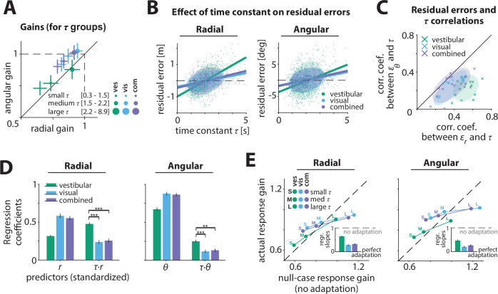
Figure 3. Effect of control dynamics on participants’ responses.
(A) Participant average of radial and angular response gains in each condition, with trials grouped into tertiles of increasing time constant τ. Error bars denote ±1 SEM. (B) Effect of time constant on radial (left) and angular (right) residual error, for an example participant (Figure 3—source data 1). Solid lines represent linear regression fits and ellipses the 68% confidence interval of the distribution for each sensory condition. Dashed lines denote zero residual error (i.e. stopping location matches mean response). (C) Correlations of radial () and angular () residual errors with the time constant for all participants. Ellipses indicate the 68% confidence intervals of the distribution of data points for each sensory condition. Solid diagonal line has unit slope. Across participants, radial correlations, which were larger for the vestibular condition, were greater than angular correlations (see also Appendix 2—table 2). (D) Linear regression coefficients for the prediction of participants’ response location (final position:, ; left and right, respectively) from initial target location (,) and the interaction between initial target location and the time constant (,) (all variables were standardized before regressing, see Materials and methods; Figure 3—source data 2). Asterisks denote statistical significance of the difference in coefficient values of the interaction terms across sensory conditions (paired t-test; *: p<0.05, **: p<0.01, ***: p<0.001; see main text). Error bars denote ±1 SEM. Note a qualitative agreement between the terms that included target location only and the gains calculated with the simple linear regression model (Figure 2B). (E) Comparison of actual and null-case (no adaptation) response gains, for radial (top) and angular (bottom) components, respectively (average across participants). Dashed lines represent unity lines, that is, actual response gain corresponds to no adaptation. Inset: Regression slopes between actual and null-case response gains. A slope of 0 or 1 corresponds to perfect or no adaptation (gray dashed lines), respectively. Error bars denote ±1 SEM.


