Abstract
Advancing diagnostic testing capabilities such as clinical next generation sequencing methods offer the potential to diagnose, risk stratify, and guide specialized treatment, but must be balanced against the escalating costs of healthcare to identify patient cases most likely to benefit from them. Heme-STAMP (Stanford Actionable Mutation Panel for Hematopoietic and Lymphoid Malignancies) is one such next generation sequencing test. Our objective is to assess how well Heme-STAMP pathological variants can be predicted given electronic health records data available at the time of test ordering. The model demonstrated AUROC 0.74 (95% CI: [0.72, 0.76]) with 99% negative predictive value at 6% specificity. A benchmark for comparison is the prevalence of positive results in the dataset at 58.7%. Identifying patients with very low or very high predicted probabilities of finding actionable mutations (positive result) could guide more precise high-value selection of patient cases to test.
Introduction
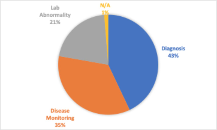
Next generation sequencing (NGS) has revolutionized research in the biological sciences and has expanded the type of medical care we can provide. NGS based testing has made it possible to detect disorders in their early stages and has opened the gateway towards precision medicine1. Ideally, such tests can be used frequently for early detection of a disorder and utilized to personalize as much of the disease management process as possible. However, with rising healthcare costs and the already overburdened healthcare system, physicians must and are striving to limit ordering to only when they are at a decision point and believe the outcome of the test will strongly affect the path they choose to go down. However, there is often too little information or too much information to synthesize when the decision has to be made. This is only further exacerbated when these tests are utilized for highly specialized clinical scenarios as is the case with the Heme-STAMP. Heme-STAMP (Stanford Actionable Mutation Panel for Hematopoietic and Lymphoid Malignancies) is a next generation sequencing based test panel. Hematopathologist often utilize Heme- STAMP for diagnostic purposes when there are hematolymphoid process where clinical, histologic, immunophenotypic, and sometimes cytogenic (FISH) information is insufficient to either render a diagnosis of malignancy, or to subtype it in a manner that is useful for sufficiently personalized clinical management. It is also used to map the progression of such disease states and to evaluate if identified laboratory abnormalities (such as cytopenias) are potentially due to hematological malignancies or something else. And is also commonly used to monitor the progression of a disease state (Figure 1). Heme-STAMP uses PCR or hybridization-based DNA capture methods alongside a “targeted sequencing” approach to detect recurrent gene fusions and to screen somatic mutation hotspots of cancer genes2.
Figure 1.
Breakdown of the most common ways Heme-STAMP is used
Given that there are a number of factors considered when determining whether to order a Heme-STAMP test, the objective of this study is to assess how well Heme-STAMP pathological variants can be predicted given electronic health records data. An accurate prediction could add the same level of informational value to care management while saving the cost of running an actual test. Because in many cases the value of the Heme-STAMP test lies in uncovering pathogenic variants, it is likely that a negative prediction will add value to the care management process while reducing the need to have the actual test ordered. A positive prediction by contrast may support the need to order the test in order to identify the specific pathogenic variants and their variant allele frequencies. Given that a negative prediction could result in not ordering the test, an inaccurate prediction might mean that a disease could bypass detection and thus progress. Because of the weight of this consequence, the negative labels were evaluated closely.
Methods
Data. A total of 2,026 Heme-STAMP clinical test results completed between June 2018 and 2020 were used. These samples were drawn from 1,743 Stanford Healthcare patients. Of these patients, 192 patients had multiple tests run over the roughly two-year period. The maximum number of tests run on a single patient was six, but the majority of these multi-test-patients (96%) had four or less tests run. Every sample in the dataset corresponds to a unique specimen. Tests for ctDNA and MRD panels were not included. All specimens underwent a routine sample quality assessment before reporting. Specimens that failed clinical quality control criteria were not included in the dataset.
These Heme-STAMP clinical test results were retrospectively combined with their respective electronic health record data from Stanford Medicine Research Data Repository (STARR)3,4. Patient features included prescribed medications, lab values of diagnostic tests, past diagnoses, demographics, and family medical history. Heme-STAMP results were overall categorized as “positive” if a pathogenic mutation was found at a variant allele frequency of <= 5% and “negative” if no pathogenic mutations were found at that variant allele frequency or if the only mutations found were variants of unknown significance (VUS).
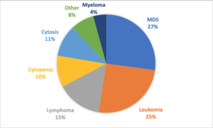
The prevalence and rate of negative results of certain diagnoses and sample types were of particular interest. As described earlier, when clinicians order the Heme-STAMP test they may have an existing diagnosis that they want to further subclassify (or check the progression of) or they may have a suspected diagnosis that the Heme-STAMP would be used to verify. Leukemia and Myelodysplastic Syndrome (MDS) are the common hematological malignancies that the clinicians are trying to monitor or evaluate as demonstrated in Figure 2. Respectively, we categorized patient populations into those with a known diagnosis of leukemia (but not of MDS), diagnosis of MDS (but not of leukemia), diagnosis of both MDS and leukemia, or no diagnosis of either disease. Patient history of diagnosis of either disease was identified from free text diagnosis summaries stored in the EHR. Because of the variety of forms and stages of leukemia and MDS, we used regular expressions (such as “%leukemia%” and “%MDS%” in various abbreviations and upper/lower case variations) to parse the diagnosis descriptions to best encapsulate patients into their correct disease categorizations. To reflect their relevance in different clinical workflows, we included specimen sample type as a key categorical feature as well.
Figure 2.
Breakdown of the most common diagnoses
Predictors. Demographic information, past diagnoses, lab orders, prescribed medications, and family histories were selected as indicator features that the model could use to predict positive or negative labels. The specific diagnoses, lab orders, prescribed medications, and family histories to use were found by selecting those that were most common among the patients in this study. These features were incorporated by indicating the presence or absence of the listed diagnoses, medications, and family histories using binary labels and by doing simple calculations to include derivatives of lab result values for each selected lab test. These derivatives were found by looking at the results of all past incidences of the specific lab test to find the minimum and maximum result values, the oldest and most recent result values, the average, the sum, and the slope across all the past lab result values. The feature values are summarized in Table 1.
Table 1.
Features/predictors used by the model
| Past Diagnoses - Leukemia, Lymphoma, Other long-term therapy, Thrombocytopenia, Neoplasm, Skin eruption, Sezary, Hypertension, Myelofibrosis, Mycosis |
| Lab Orders - WBC, Hemoglobin, RDW, MCV, Eosinophil, Monocyte, MCH, LDH, CD34, CD3PanT, CD48, CD19, Anion, IgG, Basophils, RBC, Globulin, Lymphocyte, Neutrophil, BUN, eGFR, Albumin, Glucose Serum, Calcium, Creatinine, Alkaline Phosphatase |
| Prescribed Medications - Dexamethasone, Ondansetron, Lidocaine, Heparin, Sodium Chloride, Alteplase, Epinephrine |
| Family History - Cancer, CAD, Other |
| Demographics – Sex, Age |
| Derived Features - For each numerical lab test, found patient’s maximum result values, minimum result values, average result values, sum of all result values, most recent lab value, oldest lab value, and slope of all result values |
Model Development and Specification. The primary model used was an XGBoost (eXtreme Gradient Boosting) classifier5, using a gradient boosted decision tree algorithm. This means that the model builds and aggregates the results of multiple learned decision trees in an ensemble approach to make final predictions. Instead of allowing every tree to see the entire dataset, each tree only sees a subset of the training data so that each captures a different signal which can overall be combined to have a more finely tuned model. Additionally, each tree may use a different subset of features. The subset used for each decision tree may be chosen through random selection or based on some sort of metric such as accuracy, Gini index, entropy, etc. that results as a consequence of using different subsets of features. Trees are built sequentially so that each successive tree focuses on properly classifying the observations that were misclassified by the previous tree. The model has various hyperparameters that can be adjusted, prompting us to evaluate multiple combinations: learning rate (0.01, 0.03, 0.1), n_estimater (100, 300, 600, 1000), max_depth (3, 5, 10), and subsample (0.5, 0.75, 0.9). Ultimately the following hyperparameters yielded the best results:
- N_estimators = 300 (number of decision trees used in the ensemble)
- Learning_rate = 0.03 (multiplier for the contribution of each successive classifier in the ensemble)
- Max_depth=5 (maximum depth any decision tree is allowed to have)
- Subsample = 0.5 (fraction sampled from the total dataset to build each tree)
XGBoost and Random Forest both use a decision tree algorithm but differ in how they ensemble the decision trees used. As described earlier in the paper, XGBoost Classifiers build trees sequentially. Random Forest Classifiers on the other hand build trees independently and then average the results of all the trees at the end6. To see if the unique ensemble approach of XGBoost contributed to model performance, we compared results to that of Random Forest. We trained a Scikit-Learn Random Forest classifier with the following hyperparameters7: n_estimators = 300 and max_depth = 5.
We trained a simple logistic regression model from the Scikit-Learn library in order to compare performance from decision tree-based models to linear models and experimented with sample weights inputted to the XGBoost model. As described earlier in the paper, there is a greater interest in model performance on the negative values so XGBoost models with modified sample weights were tested. Positive values were kept at a weight of 1 but weights of 1.5 and 2.5 for the negative values were experimented with. This difference in weighting would translate to greater importance placed on negative labels during the model’s training/optimization process.
In some of our initial work, we also explored LASSO (a regularization-based model) and Support Vector Machine (a max margin classifier) but found their performance to be lacking so for the rest of the study we moved forward with only the decision tree algorithms and logistic regression model described above.
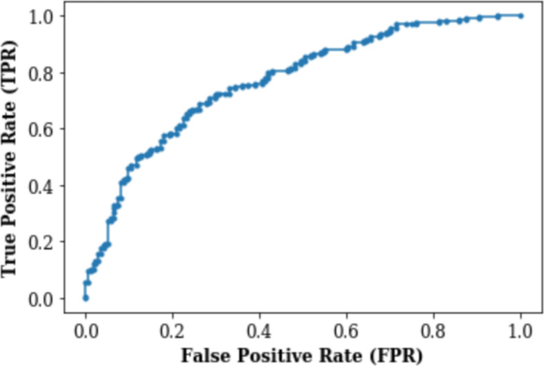
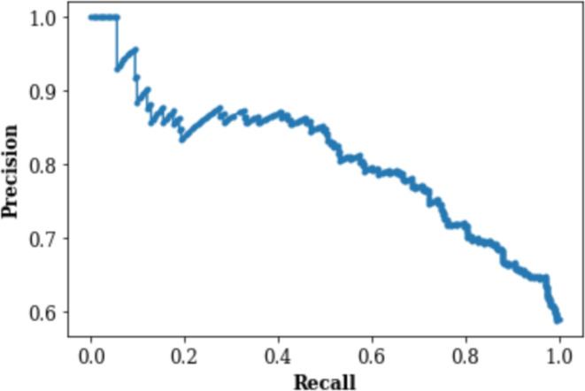
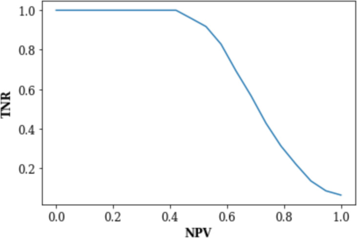
Model Evaluation. The prediction model was designed to output the pre-test probability of a positive Heme-STAMP result given all the available feature information. If the pre-test probability was greater than a certain threshold, a positive result was predicted, otherwise a negative test was predicted. The accuracy was generated based on a threshold of 0.5 but the AUROC was generated by identifying the threshold that yielded the best balance between the false positive rate and the true positive rate. The false positive rate (FPR) represents the probability that a truly negative result is predicted to be positive and the true positive rate (TPR), also known as recall or sensitivity, presents the probability that a truly positive result is predicted to be positive. The negative predictive value (NPV) and true negative rate (TNR) of these pre-test probabilities at various thresholds were used to generate the TNR vs. NPV graph. The NPV represents the probability that a predicted negative result truly is negative, and the TNR represents the probability that a truly negative result is predicted to be negative (i.e., specificity). The TPR and precision of these pre-test probabilities at different thresholds were also used to generate the Precision-Recall Curve. Precision represents the probability that a predicted positive result is truly positive (i.e., positive predictive value).
We used 10-fold stratified cross validation8 with shuffling to train and evaluate the model. For each of the 10 folds, the data was shuffled and then 90% was selected to be part of the training set and 10% to be part of the test set. The data was stratified so that each fold contained a class ratio similar to that of the overall dataset. This was to limit to the amount of class imbalance in each fold. The training dataset was used by the model to explore and learn to differentiate between samples with positive and negative labels, indicating identification or lack thereof of a pathogenic variant by Heme-STAMP testing. The test dataset was used to evaluate the performance of the now trained model on new data.
Results
The model was tested on 2,026 Heme-STAMP clinical test results using the 10-fold stratified cross validation method described above. The top 5 features were age, leukemia diagnosis, myelofibrosis diagnosis, sex, and hypertension diagnosis. Table 2 compares the performance of the random baseline and the different models: Logistic Regression, Random Forest, XGBoost (weighted), and XGBoost (unweighted). The random baseline makes only positive predictions and as expected has an accuracy equivalent to the 59% prevalence of positive test results in the dataset. All the models demonstrate accuracy levels greater than the upper limit of the 95% confidence interval for the random baseline.
Table 2.
Accuracy and AUROC with 95% Confidence Interval (C.I.) for different models and random selection
| Model | Accuracy | Accuracy 95% C.I. | AUROC | AUROC 95% C.I. |
|---|---|---|---|---|
| Random Baseline | 59% | 48-53% | ||
| Logistic Regression | 60% | 58-62% | 0.66 | 0.63-0.69 |
| Random Forest | 62% | 60-63% | 0.72 | 0.70-0.74 |
| XGBoost (unevenly weighted samples) | 69% | 67-71% | 0.74 | 0.73-0.76 |
| XGBoost | 70% | 68-71% | 0.74 | 0.72-0.76 |
Figures 3 and 4 respectively demonstrate the Receiver Operating Characteristic Curve and Precision-Recall Curve for the XGBoost model with no weighting (each class is by default weighted the same and thus effectively has no weights).
Figure 3.
Receiver Operating Characteristic (ROC) Curve
Figure 4.
Precision-Recall (PR) Curve
Among the models experimented, the weighted XGBoost had closest performance to the unweighted XGBoost model (Table 2). The main intention of the weighted XGBoost model was to see if more heavily weighting negative labels would improve the model’s performance on negative samples. So, in Table 3, we compare the NPV/TNR values of the weighted and unweighted XGBoost models to see that the values are nearly identical. The uneven weighting seems to have had no effect on the model’s performance on the negative test results. Because the NPV/TNR results are so similar, only the NPV vs TNR plot for the unweighted XGBoost model is shown in Figure 4.
Table 2.
NPV/TNR values of XGBoost weighted and unweighted models
| NPV | XGBoost TNR | XGBoost TNR (weighted samples) |
| 90% | 14% | 13% |
| 95% | 9% | 9% |
| 99% | 6% | 6% |
Table 3.
Prevalence of each subgroup in the total dataset (n = # samples), percentage of negative labels in each subgroup, and the AUROC plus the 95% confidence interval for each subgroup.
| DESCRIPTION | Prevalence in data | % Negative | AUROC | AUROC 95% C.I. |
|---|---|---|---|---|
| All | 100% (n=2,026) | 41% | 0.74 | 0.72-0.76 |
| Diagnosis | ||||
| Has leukemia diagnosis | 24.4% (n=494) | 35% | 0.70 | 0.67-0.72 |
| Has MDS diagnosis | 11.7% (n=237) | 32% | 0.71 | 0.68-0.74 |
| Has leukemia & MDS | 5.3% (n=107) | 19% | 0.63 | 0.48-0.78 |
| Has no diagnosis of leukemia or MDS | 58.6% (n=1,188) | 48% | 0.74 | 0.71-0.77 |
| Sample Type | ||||
| Bone marrow sample | 47.9% (n=970) | 44% | 0.73 | 0.70-0.76 |
| Blood sample | 42.2% (n=855) | 40% | 0.76 | 0.73-0.80 |
| Other sample | 9.9% (n=201) | 35% | 0.63 | 0.57-0.70 |
Figure 4.
Precision-Recall (PR) Curve
The prevalence and rate of negative results of diagnosis categories and sample types described in the Data section of the paper are shown in Table 3. The unweighted XGBoost model performance on these subgroups is also shown in this table. To evaluate performance, the data samples corresponding to each subgroup was identified for each fold. The AUROC for each subset was found and then averaged over all ten folds to find the average AUROC and the 95% confidence interval.
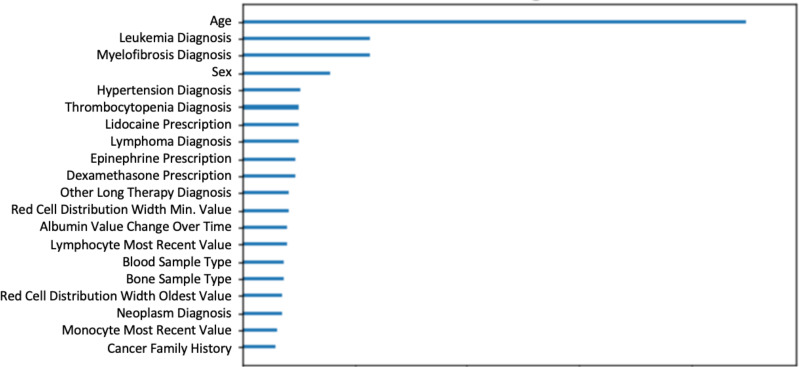
Figure 5 plots the top twenty features utilized by the unweighted XGBoost model relative to each other. A built-in feature weight function was used to identify the top twenty most important features based on the 300 decision trees fitted by the model (recall that the model was parameterized with n_estimator=300).
Figure 5.
Top twenty most important features based on trees fitted by the unweighted XGBoost Classifier
Discussion
Results and Implications. When a negative or positive result can be predicted with high accuracy, it is worth considering replacing the actual test with the predicted result since the outcomes are likely similar. And so in theory, the most high-yield diagnostic ordering strategy would be to only order tests where the predicted outcome is not able to be predicted with high accuracy. In the case of the Heme-STAMP, where it is not just the positive/negative outcome but rather the pathogenic variants detected by the test itself that matters, predicted positives should still be ordered as part of high-yield testing even if they’re predicted with high accuracy. This study sought to understand what types of features, models, and subgroups would demonstrate highest performance, especially among the negative labels. We found that the XGBoost model did best with AUROC 0.74 (95% CI: [0.72, 0.76]). Among the various subgroups, model performance was highest on the subgroup with no diagnosis of leukemia or MDS (AUROC 0.74 (95% CI: [0.71, 0.77])) and the subgroup whose specimen type was blood sample (AUROC 0.76 (95% CI: [0.73, 0.80])). And we were able to obtain 99% negative predictive value at 6% specificity.
Interpretations. In Table 2 we can see that XGBoost models (weighted and unweighted) boasted marked performance over the accuracy demonstrated by the random baseline. This shows that the model is indeed identifying patterns to make data-driven predictions. While the XGBoost models had higher accuracy than the Random Forest model, the AUROC confidence intervals greatly overlapped. This demonstrates that while XGBoost’s sequential ensemble method improved the overall accuracy of the model, this didn’t necessarily correlate to how well the model was able to differentiate between the positive and negative cases. Interestingly, while the Random Forest model had similar accuracy as the logistic regression model, all three decision-tree-based models (Random Forest, XGBoost weighted, XGBoost unweighted) had higher AUROC values than the logistic regression model did. This suggests that the ensemble tree approach is better than the linear model approach at distinguishing between classes and potentially that it takes an ensemble tree approach particularly with a sequential ensemble method to see accuracy improvement over that of a linear model.
Among the models experimented, the weighted XGBoost had closest performance to the unweighted XGBoost model (Table 2). The main intention of the weighted XGBoost model was to see if more heavily weighting negative labels would improve the model’s performance on negative samples. So, in Table 3, we compare the NPV/TNR values of the weighted and unweighted XGBoost models to see that the values are nearly identical. The uneven weighting seems to have had no effect on the model’s performance on the negative test results. Because the NPV/TNR results are so similar, only the NPV vs TNR plot for the unweighted XGBoost model is shown in Figure 4. Because the XGBoost models had the higher performance among the models but there was minimal difference between the weighted and unweighted XGBoost models, the unweighted XGBoost model was analyzed for the rest of the study.
Among cases where the physician ordered the Heme-STAMP so they could diagnose, subtype, or monitor a malignancy, leukemia and MDS were the most common such malignancies. However, we can see in Table 3 that they compose less than 50% of all the Heme-STAMP cases. Furthermore, the average negative rate across all subgroups with one or both of the malignancies is about 29% which is lower than the negative rate of the subgroup that has neither of those diagnoses. This is equivalent to saying that the average positive rate across all subgroups with one or both of the malignancies is much higher than that of the subgroup with neither diagnosis. This observation matches the clinical scenario because for patients with one or both of the malignancies, it is either known or highly likely that the patient still has the malignancy, and it is often the case that the Heme-STAMP is sought to further characterize the variants driving the malignancy. As described earlier in the paper, our model is focused on making accurate negative predictions, so it is encouraging to see that the model performance on the subgroup that has neither diagnosis and that also has the higher percentage of negative tests is closest to the overall model performance. Model performance on the subgroup with both diagnoses and on the “Other sample” subgroup is highly variable likely because of the small size of the subgroups.
In Figure 5 where we identify the top 20 features, we can see that aside from demographic information such as age and sex, biological markers such as diagnosis of leukemia and myelofibrosis were heavily utilized by the model. Both are diagnoses of hematological malignancies. Additionally, diagnoses of hypertension and thrombocytopenia indicate abnormalities with your blood circulation and blood work. Other hematological malignancies such as lymphoma and other labs related to abnormalities in blood work can be seen among these top 20 features. The model’s incorporation of these features that have clinical relevance provides assurance and credibility to the factors that the model is considering in its prediction.
Case Reviews. While we were able to reach high negative predictive values on the tests the model predicted to be negative, qualitative analysis of some of these patients highlighted some reasons why clinicians may still choose to order the test. In one such case, the clinician agreed the patient was very unlikely to have an actionable mutation, but the patient was very anxious and had the financial flexibility to take the test even if it was unlikely to be useful. In another case, the clinician had realized that the patient had a certain baseline mutation and wanted to use the Heme- STAMP to see if there were any other mutations that should be identified and used as a baseline to track changes in the patient’s condition. While some of these nuances may be grappled out free-text notes in the EHR, the complexity required to successfully do so would quickly outweigh the benefits. However, for most cases, a negative prediction from the model can actually lead to the same net information gain as an actual negative test without the cost of it. And even in nuanced cases, such as those listed above, the predicted result can still provide value to the clinician’s thought process and can serve as an additional piece of evidence to support their suggestions as they discuss various potential next step options with patients.
Earlier we described that predicted positives were of limited value because they only further supported the need to have the Heme-STAMP test run since the true value would be in the pathogenic variants the Heme-STAMP test would identify. But we found that there was some potential for positive predictions to demonstrate value. In some cases, the model predicted the result to be positive while the actual test was negative but curiously, the next Heme-STAMP test the patient took resulted in a positive outcome. In other cases, the model predicted the result to be negative while the actual test was deemed positive but a clinician looking through the report retrospectively found that the official result actually should have been negative. While more cases would have to be examined to truly extrapolate a conclusion from this observation, it still demonstrates promising potential for the model and its ability to detect underlying patterns.
Limitations. While other medical centers may also utilize next generation sequencing techniques to characterize variants, the Heme-STAMP in its exact usage is unique to Stanford’s medical center. Additionally, it hasn’t been long since the Heme-STAMP made its debut at Stanford in 2018. These factors limit the size of the sample but also reflect the cutting-edge nature of learning how to effectively use these emerging testing modalities. This study demonstrates an approach towards effective use of advanced diagnostic testing tools by developing a machine learning based tool to guide clinicians in their care management, particularly in specialized fields. In such cases the various pathways towards and stemming from a certain diagnostic test are often convoluted but imperative to understand when building and interpreting the results of a model that is intended to be implemented and not simply a proof-of-concept.
To mitigate the pitfalls of overfitting, the data was randomly split into a train/test set9 and the maximum depth of the trees and subsample ratios were kept low5. Additionally, early stopping rounds were established so that during the training process the model needed to demonstrate improvement in its evaluation metric (used log loss) every 20 rounds to continue training. This helped to ensure that the model did not continue to fit the model once it had reached a plateau in performance. The literature has shown that implementing early stopping rounds helps to keep overfitting at bay10. Due to the limitations in sample size, we allowed the model to utilize an ensemble of a high number of estimators. We balanced the cost this brought to training time by utilizing XGBoost instead of a different ensemble decision tree model because XGBoost has shown to run with better expediency than other, similar such models11.
Although sample quality and tumor content are routinely assessed before sequencing, the results may not always be accurately determined so the effect of poor sample quality on the number of negative sequencing results cannot be ruled out. However, the fact that the model can predict a subset of negative results with very high accuracy suggests that there are clinical factors characteristic to the patient’s health condition that can be learned from the electronic health record. If the majority of these negative results were due to poor sample quality, there would be no underlying factor that the model could learn from to thus make these predictions with such high accuracy.
Additionally, it is worth noting that algorithmic decision support systems such as the one described here should and can only be used to augment but never to replace clinical judgment. Only a well-trained physician can account for the complex clinical context for each individual patient. In the long-term, a combination of excellent education and data-driven tools will yield the best possible care for the greatest number of patients.
Conclusion
The objective of this paper was to see how well Heme-STAMP pathological variants could be predicted given electronic health records data. We found that by using electronic health records data readily available by the time of testing we could predict test outcome with an AUROC of 0.74 (95% CI: [0.72, 0.76]). Furthermore, we were able to identify patients that have very low probabilities of having a positive Heme-STAMP result (i.e., patients with high probability of having a negative result) and thus potential candidates for testing exclusion. These patients accounted for about 6% of all the negative tests but they could be predicted with 99% accuracy. As the number of Heme-STAMP tests ordered continues to increase, the number of patients for which we can prevent a low-yield test with high confidence will increase. This work also demonstrates promising potential to build similar prediction models for other types of Next Generation Sequencing tests. Additionally, because this predictive algorithm can also be used for patients who do not have an established diagnosis, the population it is able to provide value for will continue to grow even as we expand the use of NGS testing and reduce its cost.
Acknowledgements
We would like to thank the Stanford Pathology Department for funding this project through the Value Based Care Initiative and Kathleen Cederlof for her support through this initiative as well. We would also like to thank the Stanford Office of the Vice Provost for Undergraduate Education (VPUE) for funding this project through the VPUE Faculty Grant for Undergraduate Research. Additionally, Jonathan H. Chen’s research is supported by the NIH/National Library of Medicine via Award R56LM013365, the Gordon and Betty Moore Foundation through Grant GBMF8040, the National Science Foundation SPO181514, and the Stanford Clinical Excellence Research Center (CERC). This research used data provided by STARR, STAnford medicine Research data Repository,” a clinical data warehouse containing live Epic data from Stanford Health Care (SHC), the University Healthcare Alliance (UHA) and Packard Children’s Health Alliance (PCHA) clinics and other auxiliary data from Hospital applications such as radiology PACS. The STARR platform is developed and operated by Stanford Medicine Research IT team and is made possible by Stanford School of Medicine Research Office. The content is solely the responsibility of the authors and does not necessarily represent the official views of the NIH or Stanford Healthcare.
Figures & Table
References
- 1.Gonzalez-Garay ML. The road from next-generation sequencing to personalized medicine. Pers Med. 2014 Jul 1;11(5):523–44. doi: 10.2217/pme.14.34. [DOI] [PMC free article] [PubMed] [Google Scholar]
- 2.Sulonen A-M, Ellonen P, Almusa H, Lepistö M, Eldfors S, Hannula S, et al. Comparison of solution-based exome capture methods for next generation sequencing. Genome Biol. 2011 Sep 28;12(9):R94. doi: 10.1186/gb-2011-12-9-r94. [DOI] [PMC free article] [PubMed] [Google Scholar]
- 3.Lowe HJ, Ferris TA, Hernandez PM, Weber SC. STRIDE – An Integrated Standards-Based Translational Research Informatics Platform. AMIA Annu Symp Proc. 2009;2009:391–5. [PMC free article] [PubMed] [Google Scholar]
- 4.Wang JX, Sullivan DK, Wells AJ, Wells AC, Chen JH. Neural Networks for Clinical Order Decision Support. AMIA Jt Summits Transl Sci Proc AMIA Jt Summits Transl Sci. 2019;2019:315–24. [PMC free article] [PubMed] [Google Scholar]
- 5.Chen T, Guestrin C. XGBoost: A Scalable Tree Boosting System; Proceedings of the 22nd ACM SIGKDD International Conference on Knowledge Discovery and Data Mining [Internet]; New York, NY, USA. Association for Computing Machinery; 2016. pp. p. 785–94. [cited 2021 Mar 10]. (KDD ’16). Available from: https://doi.org/10.1145/2939672.2939785 . [Google Scholar]
- 6.Breiman L. Random Forests. Mach Learn. 2001 Oct 1;45(1):5–32. [Google Scholar]
- 7.Louppe G. Understanding Random Forests: From Theory to Practice. ArXiv14077502 Stat [Internet] 2015 Jun 3. [cited 2021 Mar 10]; Available from: http://arxiv.org/abs/1407.7502 .
- 8.Raschka S. Model Evaluation, Model Selection, and Algorithm Selection in Machine Learning. ArXiv181112808 Cs Stat [Internet] 2020 Nov 10. [cited 2021 Mar 10]; Available from: http://arxiv.org/abs/1811.12808 .
- 9.Xu Y, Goodacre R. On Splitting Training and Validation Set: A Comparative Study of Cross-Validation, Bootstrap and Systematic Sampling for Estimating the Generalization Performance of Supervised Learning. J Anal Test. 2018 Jul 1;2(3):249–62. doi: 10.1007/s41664-018-0068-2. [DOI] [PMC free article] [PubMed] [Google Scholar]
- 10.Zhang T, Yu B. Boosting with early stopping: Convergence and consistency. Ann Stat. 2005 Aug;33(4):1538–79. [Google Scholar]
- 11.Bentéjac C, Csörgő A, Martínez-Muñoz G. A Comparative Analysis of XGBoost. Artif Intell Rev. 2021 Mar;54(3):1937–67. [Google Scholar]


