A Four-Country Study on the Relationship Between Parental Educational Homogamy and Children’s Health from Infancy to Adolescence

Abstract

This study explores the relationship between parental educational similarity – educational concordance (homogamy) or discordance (heterogamy) – and children’s health outcomes. Its contribution is threefold. First and foremost, I use longitudinal data on children’s health outcomes tracking children from age 1 to 15, thus being able to assess whether the relationship changes at key life-course and developmental stages of children. This is an important addition to the relevant literature, where the focus is solely on outcomes at birth. Second, I look at different health outcomes, namely height-for-age (HFA) and BMI-for-age (BFA) z-scores, alongside their dichotomized counterparts, stunting and thinness. Third, I conduct the same set of analyses in Ethiopia, India, Peru, and Vietnam, thus providing multi-context evidence from countries at different levels of development and with different socio-economic characteristics and gender dynamics. Results reveal important heterogeneity across contexts. In Ethiopia and India, parental educational homogamy is associated with worse health outcomes in infancy and childhood, while associations are positive in Peru and, foremost, Vietnam. Complementary estimates from matching techniques show that these associations tend to fade after age 1, except in Vietnam, where the positive relationship persists through adolescence, thus supporting the homogamy-benefit hypothesis not only at birth, but also across the early life course. Insights from this study contribute to the inequality debate on the intergenerational transmission of advantage and disadvantage and shed additional light on the relationship between early-life conditions and later-life outcomes in critical periods of children’s lives.

Introduction

The relationship between parental – either mother or father’s – education and children’s health outcomes has been extensively documented across many and diverse contexts (Case & Paxson, 2002; Desai & Alva, 1998; Kemptner & Marcus, 2013; Lindeboom, Llena-Nozal, & van der Klaauw, 2009). Well-established is a positive association between mother’s educational attainment and birth-related outcomes as varied as neonatal, post-neonatal, and infant mortality (Chou, Liu, Grossman, & Joyce, 2010), birth weight (Chevalier & O’Sullivan, 2007; Currie & Moretti, 2003; Güneş, 2015), and antenatal care, postnatal care, and gestational age (Cantarutti, Franchi, Monzio Compagnoni, Merlino, & Corrao, 2017; Ruiz et al., 2015). Although the literature has focused less on the importance of father’s education, evidence also suggests that father’s education matters for children’s health (Chen & Li, 2009), yet to a slightly smaller extent (Chevalier, 2004; Cochrane, Leslie, & O’Hara, 1982).

In parallel, over the past half-century social scientists have produced an array of studies on the determinants and patterns of partners’ educational similarity or – using sociological terminology – educational assortative mating, defined as the non-random matching of partners with respect to education (De Hauw, Grow, & Van Bavel, 2017; Schwartz & Mare, 2005). While studies were mostly focused on high-income societies, more recent research has shifted gears towards low- and middle-income (LMICs) countries (Esteve, Garcia, & Permanyer, 2012; Ganguli, Hausmann, & Viarengo, 2014; Gullickson & Torche, 2014; Smits & Park, 2009). This long-standing interest in educational assortative mating is rooted in the idea that patterns of “who marries whom” matter for the reproduction of social inequalities both within and across generations (Mare, 2016; Rosenfeld, 2008). In simple terms, a society in which high-educated marry high-educated and low-educated marry low-educated will be more unequal than a society in which high-educated marry low-educated (Schwartz, 2013). Potentially, this is true both within generations – thinking, for instance, about income and wealth inequality across households (Breen & Salazar, 2011; Eika, Mogstad, & Zafar, 2019; Torche, 2010) – and cross-generationally – thinking about how heterogeneity in parental resources translates into heterogeneity of outcomes of children born to different couple “types” (Bratsberg, Markussen, Raaum, Røed, & Røgeberg, 2018).

The intersection between the above two streams of the literature – namely, the relationship between mother or father’s education and children’s health, on the one hand, and the determinants and consequences of partners’ educational similarity, on the other hand – is far less investigated. There is little evidence to date on the extent to which parental educational similarity – i.e., mother and father’s education jointly considered as a couple – is associated with children’s health, particularly in LMICs, a research question that I investigate in the present study. Scholars interested in the association between parental educational similarity and children’s health outcomes have focused exclusively on circumstances at birth or very early childhood. In one of the pioneer studies on the topic, Rauscher (2020) used administrative data on births coupled with Instrumental Variable (IV) techniques to estimate the effects of parental educational similarity on infant health – mainly birth weight, an indicator for low birth weight (LBW), and prenatal visits – in the United States. Her results suggest that parental educational homogamy is beneficial for infant health while educational hypergamy is detrimental.¹ In a similar spirit, Abufhele et al. (2020) used administrative data to look at a related research question in Chile. Their findings also suggest that parents’ educational homogamy is associated with a reduced probability of LBW and preterm birth. Both of these studies provide single-country evidence – with a focus on upper middle- and high-income societies – and children’s outcomes at birth.

To the best of my knowledge, Behrman (2019) provides the only study on the relationship of interest in a low-income context. Specifically, she explored changes overtime in the association between parental educational similarity and children’s height-for-age z-scores in Malawi, finding mother’s higher relative educational status to be negatively associated with height-for-age – contrary to the expectations of bargaining theories. Although her study looked at changes in the association between 2000 and 2015, information on children’s outcomes comes from the Demographic and Health Surveys (DHS), thus pertaining to children under the age of 5. As such, the information is not longitudinal and does not permit to track children’s health overtime. Also, in line with Rauscher (2020) and Abufhele et al. (2020), the evidence provided is from a single context.

Building on the scarce existing literature on the topic, this study seeks to provide three contributions. First and foremost, I investigate the association between parental educational similarity and children’s health using longitudinal data on children’s outcomes tracking children from age 1 to 15, thus being able to assess changes in the association at key life-course and developmental stages of children (from infancy to adolescence). Second, I look at different health outcomes, namely height-for-age (HFA) and BMI-for-age (BFA) z-scores, alongside their dichotomized counterparts (stunting and thinness, respectively). Third, I use data from the Young Lives international study of childhood poverty to conduct the same set of analyses in Ethiopia, India, Peru, and Vietnam, thus providing multi-context evidence from countries at different stages of development and with different socio-economic characteristics and gender dynamics. Due to the relevance of within-couple and gender dynamics for a research question of this kind – and the extent to which these dynamics differ by levels of countries’ development – there is reason to suspect widespread heterogeneity in the association between parental educational similarity and children’s health. The Young Lives study offers a good multi-country context to explore this heterogeneity, thus laying the ground for a more comprehensive global study on the country-level factors underlying the observed heterogeneity in the relationship between educational assortative mating and children’s health.

Results reveal important heterogeneity across contexts. In Ethiopia and India, parental educational homogamy is associated with worse health outcomes – mainly lower HFA z-scores (and higher stunting prevalence) – in infancy and childhood, while associations are positive in Peru and Vietnam. Complementary estimates from non-parametric matching techniques confirm that these associations tend to fade after age 1, except in Vietnam, where the positive relationship persists through adolescence. Compared to the relevant literature framed around the idea of benefits tied to educational homogamy, results from Ethiopia and India are particularly interesting as they are reversed in sign, corroborating the idea that family, gender, and development dynamics at the country-level interact with household-level contexts to produce an array of heterogeneous outcomes across different countries.

Insights from this study contribute to the inequality debate on the intergenerational transmission of advantage and disadvantage (persistence of inequalities versus fading) and shed additional light on the relationship between early-life conditions and later-life outcomes in critical periods of individuals’ lives – from birth to adolescence – in four distinct low- and middle-income contexts.

Background

Parental educational similarity and children’s health: Potential mechanisms

From a theoretical standpoint, parental educational similarity can affect children’s health outcomes through different channels. Family systems theory (Kerr, 2000; Minuchin, 1985) suggests that families operate as a unit, thus interactions and interrelationships among family members and their characteristics have implications for family members in current and future generations (Becker 1981; Furstenberg, 2005). One way through which educational similarity may have implications for infant health is through the prenatal context. Independently of each partner’s individual resources, educational similarity may shape prenatal conditions through maternal stress (Beck & González-Sancho, 2009; Zhang, Ho, & Yip, 2012), which in turn has implications for multiple infant health measures (Aizer, Stroud, & Buka 2016; Beijers, Jansen, Riksen-Walraven, & De Weerth, 2010; Dancause et al., 2011; Torche, 2011; Torche & Kleinhaus, 2012).

Exposure to maternal stress early in life can affect offspring outcomes via two mechanisms. First, maternal stress can negatively affect maternal behavior towards children and investments in them. Recent experimental and quasi-experimental work has shown that stress can lead to “short-sighted and risk averse decision making” (Haushofer & Fehr, 2014). Consistent with this, existing work has documented that maternal stress is correlated with less positive parenting, lower levels of cognitive stimulation, and more aggression and conflict in interactions with children (Gutman, McLoyd, & Tokoyawa, 2005; Nievar & Luster, 2006). The second mechanism is through the so-called “prenatal programming,” of which the hormone cortisol – a common marker for stress – is considered a key agent. Prenatal programming refers to “the action of a factor during a sensitive period or window of fetal development that exerts organizational effects that persist throughout life” (Seckl, 1998). Poverty is also associated with greater levels of stress, as individuals living in poverty report on average a greater number of stressful events in their lives than individuals not living in poverty (Aizer, Stroud, & Buka 2016), thus making the focus of this investigation on LMICs all the more topical.

The relationship between parental educational homogamy and child health could also be related to specific family processes or practices. For instance, homogamy could be negatively associated with maternal anxiety about her relationship with the father, and about her ability to support and care for the child after birth. In addition to relationship anxiety, educational similarity could negatively correlate with concerns related to agreement in decision-making. Parents with equal education may be more likely to agree more on parenting practices and family allocation of time and resources than parents with unequal education (Beck & González-Sancho, 2009; Martin, Ryan, & Brooks-Gunn, 2007), even controlling for each partner’s individual resources. Parental educational similarity is also typically associated with a lower likelihood of divorce (Goldstein & Harknett, 2006) and higher relationship stability (Garfinkel, Glei, & McLanahan, 2002) – which in turn influence resource-availability, within-couple decision making, and investments in children.

For the most part, these mechanisms would suggest a positive relationship between parental educational similarity and children’s health, in line with the so-called homogamy-benefit hypothesis. Although many of the aforementioned factors are most likely reflected into differential children’s outcomes at birth, due to the well-established connection between early-life and later-life health conditions (Case & Paxson, 2010), there is reason to believe differential outcomes might persist through adulthood. As mentioned above with reference to prenatal programming, there is solid scholarly work that relates stress in the prenatal period with worse child outcomes both in infancy and in later life. For instance, using sibling data, Aizer, Stroud, & Buka (2016) found in-utero exposure to elevated levels of the stress hormone cortisol to negatively affect birth outcomes (gestation and birth weight), as well as IQ and child health at age 7, ultimately leading to lower educational attainment as adults. Similarly, Persson & Rossin-Slater (2018) found that in-utero exposure to maternal stress from family rupture affects mental health both during childhood and in adulthood. In general terms, even if we expected prenatal stress to reflect itself more into negative outcomes in the postnatal period and during infancy, there are plenty of other mechanisms discussed above – such as agreement on parenting practices, family instability, decisions regarding resource-allocation – that function over a longer and continuous time span, and are therefore likely to have long-lasting influence on children’s health trajectories. The focus of this study on health trajectories of children in both childhood and early adolescence rests precisely on these premises.

Cross-country heterogeneity and variation

This study focuses on selected sentinel sites in Ethiopia, India, Peru, and Vietnam, four different countries with their own socio-economic characteristics, cultural specificities, norms, and traditions. Although a thorough description of these countries and their characteristics is beyond the scope of this study, it is nonetheless key to shed some light on a set of country-specific factors that – alone or in tandem – might underlie the relationship between parental educational similarity and children’s health across the four LMICs. As a matter of fact, while the above theoretical perspectives lead to the expectation that parental educational similarity might be beneficial for children’s health both at birth and through adulthood (homogamy-benefit hypothesis), this might not be the case in all contexts and might actually hinge upon specific country characteristics. A four-country study of this kind provides a good initial setting to assess between-country variability and speculate – if not test directly – as best as possible on which factor(s) might be playing the strongest role. Table 1 categorizes these features under four labels, namely “education,” “family,” “gender,” and “development” and provides nationally-representative estimates of some characteristics drawn from sources such as the World Bank Development Indicators (WDI), the United Nations Development Programme (UNDP), or the Demographic and Health Surveys (DHS). All estimates refer to year 2002 – the birth year of children in the Young Lives study – or the closest available year.

Table 1:

Country-level characteristics that may underlie the relationship between parental educational homogamy and children’s health, by country (around year 2002)

	a. Education			b. Family		c. Gender				d. Development
	Mean years of schooling (male)	Mean years of schooling (female)	School enrollment, primary and secondary (gross), gender parity index	Prevalence of arranged marriage	Age difference between spouses (husband-wife)	Within society			Within couples	Human Development Index (HDI)	GDP per capita (current US$)
						Global Gender Gap (GGG)	Gender Development Index (GDI)	Gender Inequality Index (GII)	% of couples where husband is sole decision maker on money
Ethiopia	2.1	0.9	0.657	Medium-High	9.11	0.595	0.741	0.614	8.08	0.306	111.9
India	6.2	3.2	0.802	High	6.12	0.601	0.738	0.629	27.24	0.508	471
Peru	8.9	7.6	0.982	No	4.01	0.662	0.915	0.461	1.86	0.688	2,021.20
Vietnam	5.9	5.0	0.925	Low	2.87	0.689	0.956	0.317	16.65	0.594	430.1

Notes: Mean years of schooling, male: UNDP, 2000; Mean years of schooling, female: UNDP, 2000; School enrollment, primary and secondary (gross), gender parity index (GPI): World Bank, 2000; Prevalence of arranged marriage: Pesando and Abufhele (2019) and Corno, Hildebrandt, and Voena (2020); Age difference between spouses: DHS for Ethiopia from 2000; DHS for India from 1998; DHS for Peru from 2000; DHS for Vietnam from 2002. Weighted estimates; Global Gender Gap: World Economic Forum, 2006 (the higher the better); Gender Development Index: UNDP, 2002 (higher index, less discrepancies between men and women); Gender Inequality Index: UNDP, 2005 (higher index, higher inequality); % couples where the husband is the sole decision maker on money issues: DHS for Ethiopia from 2000; DHS for India from 1998; DHS for Peru from 2000; DHS for Vietnam from 2002. Weighted estimates; HDI: UNDP year 2002; GDP per capita: World Bank, 2002.

Starting from education (panel a), estimates of mean years of schooling are very different across countries, lowest in Ethiopia for both males (2.1) and females (0.9) and highest in Peru (8.9 and 7.6, respectively). The comparison between males and females’ years of education reflects stark gender inequalities, particularly in Ethiopia and India, while Vietnam is close to parity in mean years of schooling. These inequalities are also reflected in the gender parity index for primary and secondary school enrolment, which is close to 1 in Peru and Vietnam, while it is 0.802 in India and 0.657 (i.e., far from parity) in Ethiopia. Variation in aggregate education levels across countries is perhaps the most immediate factor underlying heterogeneity in the relationship between parental educational similarity and children’s health. The most obvious reason is that aggregate education levels (or educational distributions of women and men) affect the likelihood of forming educationally-homogamous couples, as further discussed in the subsequent sections. An additional country-level factor falling under the education umbrella which possibly matters for the relationship of interest is the share of students in single-sex education versus co-education. By separating boys and girls into different schools during school years, single-sex schools limit the opportunities for students to develop interpersonal relationships with students of the opposite sex and to meet their potential spouses in school. Although I could not find reliable nationally representative estimates of the share of children in single-sex schools, ancillary sources suggest that co-education remains the norm in these countries. It is therefore unlikely for this to be a driving factor of cross-country variability.

In the family panel (b) I consider two variables which previous research has relied upon to measure traditional customs and patriarchal norms in low-income contexts, namely parental control over marriage (i.e., the extent to which couples are formed “freely” versus they are arranged) and the age difference between spouses (Pesando, 2021; Casterline, Williams, & McDonald, 1986). Casterline, Williams, & McDonald (1986) claimed that in patriarchal societies and in societies characterized by patrilineal kinship organizations, the spousal age difference tends to be relatively large. Conversely, in settings where the traditional social structure allows for a more equal status of spouses, or where exposure to Western family forms and modernization processes have improved the status of women, the age difference tends to be smaller. Table 1 suggests that these differences are highest in Ethiopia (9 years), followed by India (6), Peru (4) and Vietnam (2.9), thus suggesting more unequal status of spouses in the former two countries. Ethiopia and India are also the countries where arranged marriage remains more prevalent (Pesando and Abufhele 2019; Corno, Hildebrandt, & Voena, 2020). On the one hand, the practice of arranged marriage might be associated with the formation of educationally-homogamous couples, as partners are selected purposively by parents – or jointly by parents and children – from a limited and selected pool of individuals. If the homogamy-benefit hypothesis applies, this might be associated with improved child outcomes. On the other hand, contexts where arranged marriage is prevalent and the age difference between spouses is wide tend to be more gender-unequal, thus making the relationship between parental educational similarity and children’s health more complex.

In this respect, the third panel focuses on gender dynamics (c) both within societies and within couples. I rely on indicators such as the Global Gender Gap (GGG) from the World Economic Forum (WEF), the Gender Development Index (GDI) and the Gender Inequality Index (GII) from the UNDP, and the share of couples where the husband is the sole decision maker on money-related decisions computed from DHS. Irrespective of society-level indicators, Ethiopia and India have almost the same scores in terms of GGG, GDI, and GII, which are far worse than scores for Peru and Vietnam. However, data show that gender dynamics within couples are more unequal in India than Ethiopia, with 27 percent of male partners making decisions about money matters solely on their own. Vietnam ranks as the most gender equal country among the four, with a GII as low as 0.32 (half its value for Ethiopia and India). Dynamics of gender inequality matter importantly for explaining cross-country variation in the relationship investigated in this study. I hypothesize that in contexts with rooted gender inequalities within societies and within couples, the potential benefits of parental educational similarity for children’s health (e.g., less stress, more agreement on parenting practices, more balanced allocation of resources, etc.) might be offset and even reversed as male partners might feel threatened by status homogamy.

Lastly, panel d considers measures of socio-economic or human development, namely the Human Development Index (HDI) and GDP per capita, which are deeply intertwined with all the variables discussed hitherto (for instance, the HDI includes mean years of schooling in its computation). Also according to these variables, Ethiopia has the lowest values of HDI and GDP per capita, while Peru has the highest values of both. According to both variables, Ethiopia is the least developed country, far less developed than India itself. Considering all factors together, we could summarize data in Table 1 as describing two sets of countries, with Ethiopia and India scoring more poorly across the majority of indicators and Peru and Vietnam scoring better. Within the first group of countries, socio-economic development is lower in Ethiopia, yet gender inequalities and family practices such as arranged marriage are more prevalent in India. Within the second group of countries, socio-economic development and mean years of schooling are higher in Peru, yet gender inequalities are lower in Vietnam.

Drawing on the idea that education, family, gender, and development characteristics at the country level interact with each other to produce an array of different outcomes, I expect the association between parental educational similarity and children’s health outcomes to be more similar between Ethiopia and India, as well as between Peru and Vietnam. As the aforementioned country characteristics of Peru and Vietnam are more similar to those of Chile and the United States (compared to those of Ethiopia and India) – the countries in which similar investigations have been conducted and evidence for the homogamy-benefit hypothesis has been found (Abufhele et al. 2020; Rauscher, 2020) – I expect to find evidence in favor of the homogamy-benefit hypothesis in these two countries. As for Ethiopia and India, hypotheses are less clear-cut, yet there is reason to expect the low levels of development and stark gender inequalities to “neutralize” or weaken the beneficial effects of parental educational similarity for child health.

Data and variables

Dataset and study design

I analyze data from five waves of the Young Lives (YL) international study of childhood poverty, which follows the lives of children in four countries – Ethiopia, India, Peru, and Vietnam – in 2002 (Barnett et al., 2013). The present analysis uses data from the younger cohort, with children between 6.0 and 17.9 months at recruitment (mean 11.7 months). Follow-up data were collected in 2006 (mean 5.3 y), in 2009 (mean 7.9 y), 2013 (mean 12.0 y), and 2016 (mean 15.0 y). In the study, I refer to the survey rounds by referring to children’s mean ages in years – 1, 5, 8, 12, and 15, respectively.

In each study country, participants were selected through a multi-stage sampling process beginning with 20 sentinel sites that were purposively selected to reflect the study’s aims of examining the causes and consequences of childhood poverty and diversity of childhood experiences, with oversampling of sites covering poor areas (Wilson & Huttly, 2004). In India, recruitment was restricted to the state of Andhra Pradesh, which subsequently divided into two states, Andhra Pradesh and Telangana. Within each sentinel site, approximately 100 children within the eligible age category were randomly sampled, with one study child per household (Barnett et al., 2013). The exact procedures used varied between sites because of topographical and administrative differences within and between countries but was carefully documented to ensure a sample indistinguishable from one drawn at random from qualifying households, with reasonable control of bias (Wilson & Huttly, 2004). Less than 2 percent of selected households refused to participate. The low refusal rates might be explained by the involvement of local fieldworkers of both sexes and different ethnicities that facilitated acceptance by the communities (Barnett et al., 2013). Comparisons with children in the nationally representative Demographic and Health Surveys found the Young Lives samples to cover a broad diversity of children within each country (Young Lives, 2017). Data are unweighted, as typically done in analyses using the YL dataset.

Anthropometric outcomes

I focus on the following anthropometric measures of infant, child, and adolescent health: height-for-age (HFA) and BMI-for-age (BFA) – and the respective dichotomized indicators for stunting and thinness. Health outcomes were recorded longitudinally at five time points and were not self-reported. Children in the younger cohort had their heights measured and were weighed when they were aged between 6 and 17 months, and repeatedly in subsequent rounds. Child height was measured to the nearest 0.1 cm using height boards made for the purpose. Child weight was measured using calibrated child scales and recorded to the nearest 0.1 kg (Petrou & Kupek, 2010). The above outcomes were obtained combining these measurements with the age of the child in days, a variable that was not made publicly available (Briones, 2018). Using the World Health Organization (WHO) 2006 reference standards for assessing growth and development of children (World Health Organization, 2006) and the WHO Growth References (De Onis et al., 2007) for children older than 60 months (school-aged and adolescents), children were further classified as stunted and thin if they had an HFA z-score<−2 standard deviations (SD) and a BFA z-score<−2 SD, respectively. I therefore look at two outcomes per dimension:

• Height-for-age (HFA): HFA z-score (continuous) and stunting (dichotomous)

• BMI-for-age (BFA): BFA z-score (continuous) and thinness (dichotomous)

The focus on z-scores on top of the more conventional nutritional thresholds (such as stunting) is widely supported in the literature (Headey, Hoddinott, Ali, Tesfaye, & Dereje, 2015; Kumar & Singh, 2013) and justified by the idea that continuous measures capture changes over the whole distribution rather than at one point only. Other studies in the YL context have relied on these same outcomes (e.g., Anand, Behrman, Dang, & Jones, 2018; Georgiadis et al., 2017; Petrou & Kupek, 2010; Schott, Crookston, Lundeen, Stein, & Behrman, 2013).

HFA is the most prevalent measure of accumulated undernutrition, infection, and impaired growth and development since – and even before – birth (De Onis & Branca, 2016). This measure can therefore be interpreted as an indication of poor environmental conditions or long-term restrictions of a child’s growth potential. On a population basis, high levels of stunting are associated with poor socioeconomic conditions and increased risk of frequent and early exposure to adverse conditions such as illness and/or inappropriate feeding practices (World Health Organization, 2006). BFA measures weight adjusted for height and age, and is a widely-adopted variable to track childhood obesity (Cole, Flegal, Nicholls, & Jackson, 2007). BFA is often preferred to weight-for-length for children older than 2, but it is now also used to monitor growth in children younger than 2 – so that there is no need to switch between variables when tracking growth from birth to adulthood (Furlong et al., 2016). As I track children from early childhood to adolescence, I follow this same approach, focusing on BFA rather than weight-for-length.

While the YL study also reports data on weight-for-age (WFA) and prevalence of underweight (defined as a WFA z-score <−2SD), these variables were only recorded in the first three rounds of data, i.e., up to age 8, as the WHO reference tables are applicable only to children of certain ages (Briones, 2018). Also, WFA reflects weight relative to chronological age, thus being influenced by both the height of the child (height-for-age) and his/her weight (weight-for-length). For instance, WFA fails to distinguish between short children of adequate body weight and tall and thin children. As its composite nature makes interpretation complex, I decided to focus the main analyses on HFA and BFA, while supplementary analyses on WFA for the first three rounds of data are reported in the Appendix. Appendix Table A.1 reports correlation coefficients between these outcomes, supporting the idea that the correlations between HFA and WFA on one hand, and BFA and WFA on the other hand, are substantial – therefore only focusing on HFA and BFA might be a sensible strategy.

Parental educational similarity

The main predictor of interest is parental educational similarity, i.e., the extent to which the father and the mother of the YL child have the same (concordance or educational homogamy) or different (discordance or educational heterogamy) level of education. I construct this variable as the difference in grade attained between the father and the mother as recorded in wave 1. As I am interested in parental educational similarity in the prenatal period, parental education recorded when the child was age 1 provides the best proxy. If the difference is zero, the couple is coded as educationally homogamous; if the difference is different from zero, the couple is coded as educationally heterogamous.² As robustness check, I also compute the main predictor of interest using parents’ education coded in categories according to country-specific thresholds of lower and upper primary and lower and upper secondary education (in a spirit similar to Reynolds et al., 2017). Respondents who indicated that they were literate but had not participated in any formal schooling were assigned to the incomplete lower primary schooling level. Schooling levels were coded with integer values 0–9, where 0 corresponds to “No Schooling,” 1 “Incomplete lower primary,” 2 “Lower primary complete,” 3 “Incomplete upper primary,” 4 “Upper primary complete,” 5 “Incomplete lower secondary,” 6 “Lower secondary complete,” 7 “Incomplete upper secondary,” 8 “Upper secondary complete,” and 9 “Some tertiary education.”³ With these categories, I identify if the couple is homogamous by taking the difference in levels, following the same logic adopted for the continuous variable.

While missing data on mother’s education were minimal – ranging from 0.5 to 2 percent across countries – father’s education was more often missing (descriptive statistics on predictors in wave 1 are reported in Table 2), especially in Ethiopia and Peru, likely due to mortality or migration dynamics that are beyond the scope of this study. Specifically, the share of missing data for father’s education is 12.6, 0.8, 15.2, and 3.6 percent in Ethiopia, India, Peru, and Vietnam, respectively. This is an important issue to the extent that it does not permit to obtain a couple-level measure of educational similarity. In the analyses that follow, I exclude couples with missing information on either parent’s education, yet I conduct sensitivity analyses in Ethiopia and Peru by bounding the estimates – i.e., assuming all missing couples to be either homogamous or heterogamous – to show that missing couples do not strongly affect the observed associations between educational homogamy and children’s health.

Table 2:

Summary statistics on predictors of interest as of round 1 (R1; 2002)

	Ethiopia			India
	Obs.	Mean	(SD)	Obs.	Mean	SD
Child is female (Ref.: Male)	1,803	0.470	(0.499)	1,891	0.462	(0.499)
Age of the child (months)	1,803	11.67	(3.572)	1,891	11.83	(3.481)
Mother’s (M) grade attained	1,783	2.324	(3.557)	1,884	2.959	(4.169)
Father’s (F) grade attained	1,576	3.026	(4.094)	1,875	4.427	(4.851)
F-M difference in grade	1,570	0.823	(4.150)	1,871	1.475	(4.061)
Average parental grade attained	1,570	2.628	(3.531)	1,871	3.690	(4.040)
Mother’s age	1,788	27.41	(6.430)	1,885	23.66	(4.362)
Father’s age	1,589	36.45	(9.065)	1,879	29.43	(5.213)
F-M difference in age	1,582	8.857	(6.092)	1,875	5.773	(2.877)
Child’s birth order	1,803	3.179	(2.009)	1,891	1.702	(0.994)
Number of siblings	1,803	2.189	(2.013)	1,891	0.710	(1.009)
Share of female siblings	1,803	0.367	(0.376)	1,891	0.245	(0.405)
Household size	1,803	5.765	(2.150)	1,891	5.446	(2.366)
Household is in urban area (Ref.: Rural)	1,803	0.339	(0.473)	1,891	0.238	(0.426)
	Peru			Vietnam
	Obs.	Mean	(SD)	Obs.	Mean	SD
Child is female (Ref.: Male)	1,807	0.496	(0.500)	1,891	0.488	(0.500)
Age of the child (months)	1,807	11.54	(3.525)	1,891	11.65	(3.166)
Mother’s (M) grade attained	1,768	7.140	(4.509)	1,878	5.523	(4.110)
Father’s (F) grade attained	1,533	8.258	(4.210)	1,822	6.081	(4.139)
F-M difference in grade	1,518	1.138	(3.689)	1,812	0.520	(3.670)
Average parental grade attained	1,518	7.703	(3.983)	1,812	5.817	(3.695)
Mother’s age	1,802	26.90	(6.785)	1,890	27.13	(5.758)
Father’s age	1,608	30.81	(7.615)	1,844	30.04	(5.989)
F-M difference in age	1,608	3.612	(4.999)	1,844	2.969	(3.179)
Child’s birth order	1,807	2.303	(1.646)	1,891	1.825	(1.030)
Number of siblings	1,807	1.312	(1.648)	1,891	0.829	(1.032)
Share of female siblings	1,807	0.284	(0.392)	1,891	0.294	(0.434)
Household size	1,807	5.710	(2.337)	1,891	4.901	(1.841)
Household is in urban area (Ref.: Rural)	1,807	0.682	(0.466)	1,891	0.183	(0.387)

Notes: F: father; M: mother.

Other variables

The study includes additional variables as controls, namely child’s sex, child’s birth order, child’s ethnic group, number of siblings that are younger than the YL child,⁴ share of siblings who are female, mother’s age, household location of residence (rural versus urban), and region of residence. Importantly, all analyses control for mother and father’s individual levels of education (grade attained). This is key to ensure that any “homogamy effect” does not simply reflect higher (or lower) maternal or paternal “individual” resources. All controls are wave-specific – i.e., they are allowed to vary over waves in the analysis – except for the time-invariant ones, namely child sex, birth order, and ethnic group of the child. As the YL study is focused on the lived experiences of children, few other variables on parents are present in the dataset.

Sample

The analytical sample consists of children who were present in all five survey rounds (N=7,392, all countries combined). Out of the total number of children surveyed in round 1 (N=8,062), this represents 91.7 percent of the original sample (90.2 percent in Ethiopia, 94 percent in India, 88.1 percent in Peru, and 94.6 percent in Vietnam). Appendix Table A.2 provides attrition analyses comparing characteristics of children in the analytical sample with those of children who left the study in any round following the first. Children in urban areas were significantly more likely to attrite in all countries except for Peru. Also, in Ethiopia and Vietnam parents of children who left the study had significantly higher schooling. As this study focuses on a couple-level measure of educational concordance and these differences are observed similarly for mothers and fathers, this finding should not pose threats to the validity of the estimates. Furthermore, no systematic differences in anthropometric outcomes were observed across the two groups, suggesting that children who left the study were not suffering from significantly poorer health.

Methodology

My methodological approach proceeds as follows. First, I run a series of Ordinary Least Squares (OLS) regressions predicting anthropometric outcomes at ages 1, 5, 8, 12, and 15. As the samples are not nationally representative, I conduct separate analyses by country, rather than pooling the samples together, as typically done with studies using YL data. I run three models for each outcome: one with no controls (NC), one adding controls for mother and father’s education measured continuously (EDU) and one with the full set of controls listed above (FULL), specifically child’s sex, age, ethnic group, birth order, number of younger siblings, share of siblings who are female, mother’s age, mother and father’s education, household location of residence, and region of residence.⁵ Standard errors are clustered at the cluster (sentinel-site) level.

Second, I move beyond OLS by employing a series of non-parametric matching models. Non-parametric matching models have two distinct advantages over regression-based models: they do not assume any a priori functional form for the relationship between parental educational similarity and children’s health outcomes, and they rely on comparing (or “matching”) the treatment observations with a closely matched set of control observations rather than using all the untreated observations in the sample as controls, some of which are simply not comparable. Indeed, like OLS, non-parametric matching models assume that selection into educationally-homogamous couples is based only on observable characteristics and is therefore exogenous to children’s outcomes, conditional on including these controls. For this reason, no claim of causality is made throughout the analysis. The observable characteristics that are used to predict the probability of observing an educationally-homogamous couple are mother’s age, father’s age, mother’s education, father’s education, the number of people living in the community, and the average distance between the community and the district/regional capital. The latter two variables are included to proxy for some sort of marriage-market information. Matching is carried out by country and household location of residence (rural/urban). I run two specifications, one with nearest-neighbor matching with 1 match and caliper 0.1 – labelled “C(0,1),” and another with nearest-neighbor matching with 4 matches – labelled “NN(4).”

Descriptive statistics on parental educational similarity and children’s health

Table 3 provides summary statistics on the prevalence of homogamy and heterogamy – further subdivided into hypogamy and hypergamy – by country of study. To show consistency, parental educational similarity is categorized using two different criteria: schooling as grade attained (top panel) and schooling in country-specific categories (10 categories, bottom panel). As such, when obtaining homogamy estimates, the first classification is more stringent – the estimate for the share of homogamous couples is lower – while the second classification is less stringent. Results are interpreted with reference to the continuous classification (top panel), yet findings using the less stringent classification are in line and consistent. Summary statistics from Table 3 suggest that the share of homogamous couples is higher in Ethiopia and India – 0.57 and 0.49, respectively – and lower in Peru and Vietnam – 0.25 and 0.37, respectively. Vietnam is the country with the highest share of hypogamous couples, i.e., couples in which the mother has higher education than the father. The estimate is 0.26, closely followed by Peru (0.25). Overall, couple educational composition is rather similar in Ethiopia and India, and quite similar in Peru and Vietnam, with the difference in the latter two countries being that hypergamy is more prevalent in Peru.

Table 3:

Summary statistics on the prevalence of homogamy and heterogamy, by country

Share of couples (R1)	Ethiopia	India	Peru	Vietnam
	Education (grade attained)
Homogamous (M=F)	0.573	0.494	0.250	0.368
Heterogamous	0.427	0.506	0.750	0.632
Hypergamous (M<F)	0.303	0.377	0.498	0.375
Hypogamous (M>F)	0.124	0.129	0.252	0.257
	Education (ten categories)
Homogamous (M=F)	0.588	0.528	0.374	0.402
Heterogamous	0.412	0.472	0.627	0.598
Hypergamous (M<F)	0.295	0.351	0.419	0.358
Hypogamous (M>F)	0.117	0.121	0.208	0.240

Notes: R1: Round 1; M: Mother; F: Father.

As discussed above, the educational distributions of these four countries are vastly different. Therefore, it is likely to expect educational homogamy to be distributed differently across groups. For instance, in a country like Ethiopia in which the majority of mothers and fathers are in the “No schooling” or “Incomplete lower primary” categories, the likelihood of an educationally-homogamous pairing forming at the bottom of the educational distribution is higher than, for instance, in Vietnam. Figure 1 provides the distribution of educational homogamy – i.e. the share of mothers (top) and fathers (bottom) in educationally-homogamous couples – by mother and father’s levels of education in categories. The figure shows that educational homogamy tends to occur more often at the bottom and the top of the educational distribution in Ethiopia and India, while less so in Peru and Vietnam.⁶ Overall, Peru is the country with the most even (or least “skewed”) distribution among the four. For instance, in Ethiopia, India, and Vietnam, among mothers with no schooling, 77, 68, and 55 percent were in homogamous couples, respectively, while this estimate decreases to 16 percent in Peru. Similarly, in Ethiopia, India, and Vietnam, among fathers with no schooling 90, 86, and 66 percent were in homogamous couples, respectively, while this estimate decreases to 49 percent in Peru.

Figure 1:

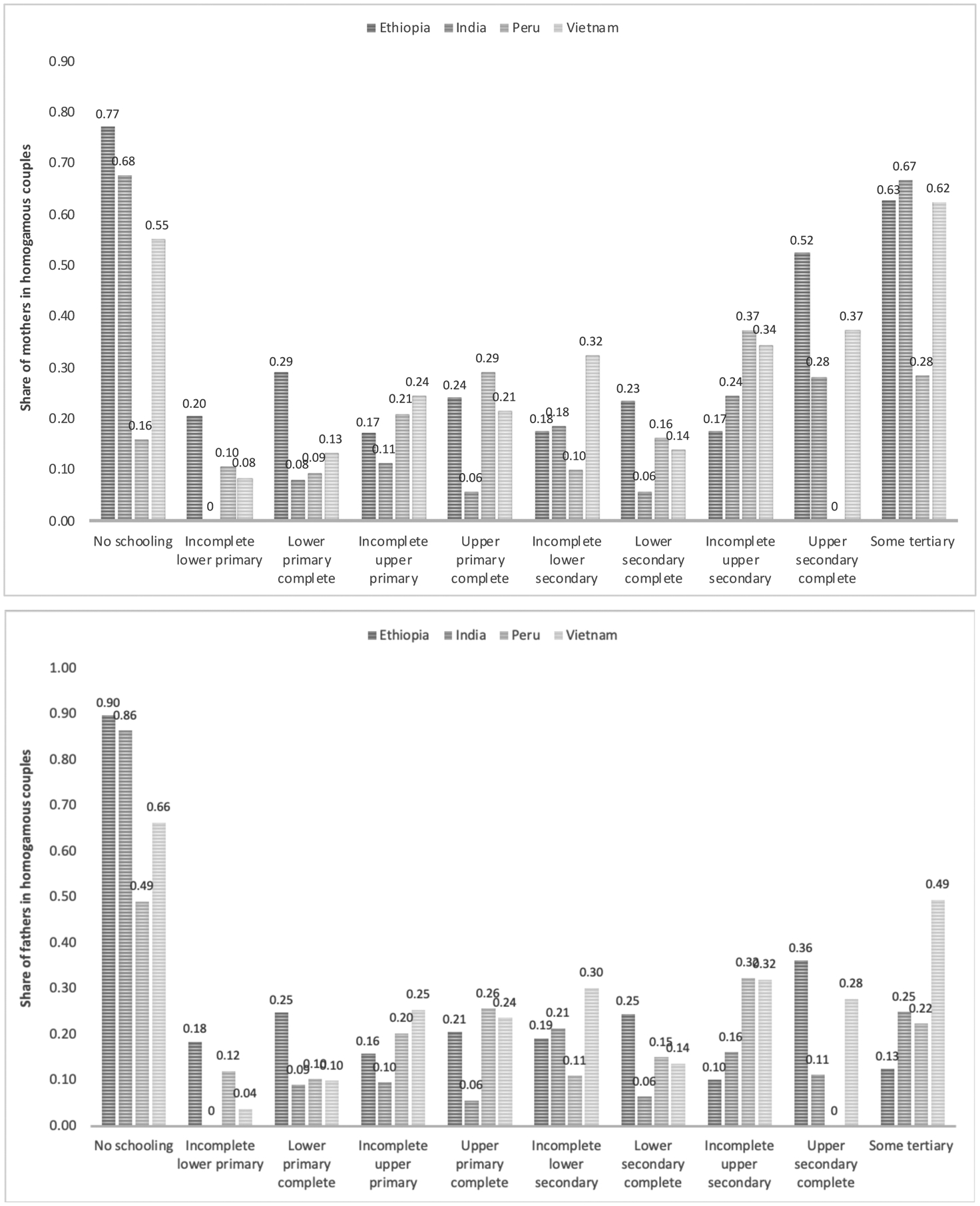
Distribution of educational homogamy, by mother (top) and father’s (bottom) levels of education, by country

To provide further evidence of differences in the distribution of educational homogamy between countries, Figure 2 describes the share of educationally-homogamous couples by terciles of average parental education, computed as the mean between the continuous variable (grade attained) for mother and father’s education. Both Ethiopia and India stand out from this graph as the data reveal that in the lowest tercile of average parental education, all couples (100 percent) are educationally homogamous, while less than 20 percent of couples are homogamous within the middle and top terciles.

Figure 2:

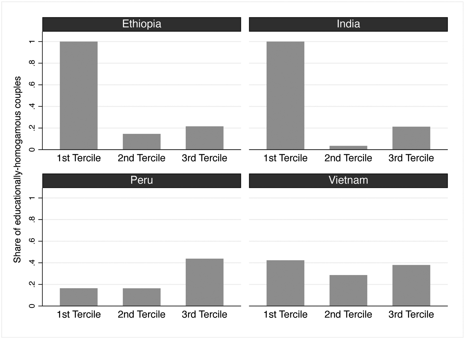
Distribution of educational homogamy by average parental education terciles, by country

Table 4 provides descriptive statistics on children’s anthropometric outcomes by country and age of the child (i.e., round of the survey). Starting from Ethiopia, YL data suggest that about 40 percent of children are stunted at age 1, and this estimate declines with age, down to 26 percent of adolescents stunted at age 15. Conversely, 15 percent of children are thin at age 1, while prevalence increases with age reaching 36 percent at age 15. Trends for the two variables are similar in India, with one difference: stunting, although declining with age, is less prevalent to start with (30 percent of children at age 1 compared to 40 percent in Ethiopia). A similar share of adolescents (28 percent) is stunted at age 15. Thinness also becomes more prevalent with age. In Peru and Vietnam, stunting is less prevalent and declining with age. Prevalence of thinness is very low in Peru – no more than 1 percent of children – and a little higher in Vietnam – between 1 and 3 percent – though far lower than in Ethiopia and India. Overall, anthropometric outcomes and changes across ages are more similar between Ethiopia and India, as well as between Peru and Vietnam.

Table 4:

Summary statistics on children’s anthropometric outcomes, by country and age of the child (wave)

			Ethiopia (N=1,803)					India (N=1,891)
			Age 1	Age 5	Age 8	Age 12	Age 15	Age 1	Age 5	Age 8	Age 12	Age 15
Height-for-age (HFA)	HFA z-score	Mean	−1.536	−1.449	−1.185	−1.460	−1.323	−1.333	−1.645	−1.428	−1.463	−1.474
		(SD)	(1.943)	(1.121)	(1.185)	(0.995)	(1.105)	(1.613)	(1.118)	(1.187)	(1.102)	(1.039)
	Stunting (<−2 SD)	Mean	0.411	0.310	0.210	0.289	0.256	0.305	0.360	0.293	0.293	0.277
		(SD)	(0.492)	(0.462)	(0.407)	(0.453)	(0.436)	(0.461)	(0.480)	(0.455)	(0.455)	(0.448)
BMI-for-age (BFA)	BFA z-score	Mean	−0.669	−0.621	−1.312	−1.818	−1.610	−1.034	−1.175	−1.415	−1.359	−1.138
		(SD)	(1.525)	(1.095)	(1.059)	(1.002)	(1.161)	(1.172)	(1.024)	(1.196)	(1.510)	(1.345)
	Thinness (<−2 SD)	Mean	0.154	0.083	0.212	0.413	0.363	0.192	0.187	0.273	0.331	0.255
		(SD)	(0.361)	(0.275)	(0.408)	(0.492)	(0.482)	(0.394)	(0.390)	(0.445)	(0.471)	(0.436)
			Peru (N=1,807)					Vietnam (N=1,891)
			Age 1	Age 5	Age 8	Age 12	Age 15	Age 1	Age 5	Age 8	Age 12	Age 15
Height-for-age (HFA)	HFA z-score	Mean	−1.279	−1.548	−1.158	−1.035	−1.198	−1.126	−1.347	−1.107	−1.057	−1.026
		(SD)	(1.340)	(1.155)	(1.056)	(1.167)	(1.132)	(1.327)	(1.105)	(1.064)	(1.153)	(0.929)
	Stunting (<−2 SD)	Mean	0.276	0.329	0.201	0.185	0.160	0.208	0.257	0.201	0.196	0.124
		(SD)	(0.447)	(0.470)	(0.401)	(0.388)	(0.367)	(0.406)	(0.437)	(0.401)	(0.397)	(0.330)
BMI-for-age (BFA)	BFA z-score	Mean	0.787	0.682	0.514	0.527	0.410	−0.410	−0.317	−0.687	−0.623	−0.564
		(SD)	(1.324)	(1.054)	(1.061)	(1.123)	(0.964)	(0.979)	(1.110)	(1.396)	(1.279)	(1.187)
	Thinness (<−2 SD)	Mean	0.022	0.004	0.009	0.010	0.008	0.038	0.038	0.119	0.139	0.104
		(SD)	(0.148)	(0.067)	(0.094)	(0.097)	(0.088)	(0.192)	(0.191)	(0.323)	(0.346)	(0.306)

Results

OLS estimates

Figure 3 provides results on the relationship between parental educational homogamy and children’s outcomes at the five different ages. I present results on the four outcomes for each country separately. In the figure, only the coefficient of parental educational homogamy is reported. The light grey marker refers to the estimated coefficient without controls (NC), the dark grey marker refers to the estimated coefficient controlling for mother and father’s education (EDU), while the black marker refers to the estimated coefficient after including all controls (FULL). The longest bar corresponds to a 99 percent confidence interval, while the more solid line within each bar refers to a 95 percent confidence interval. Corresponding estimates and standard errors are reported in Appendix Table A.3.

Figure 3:

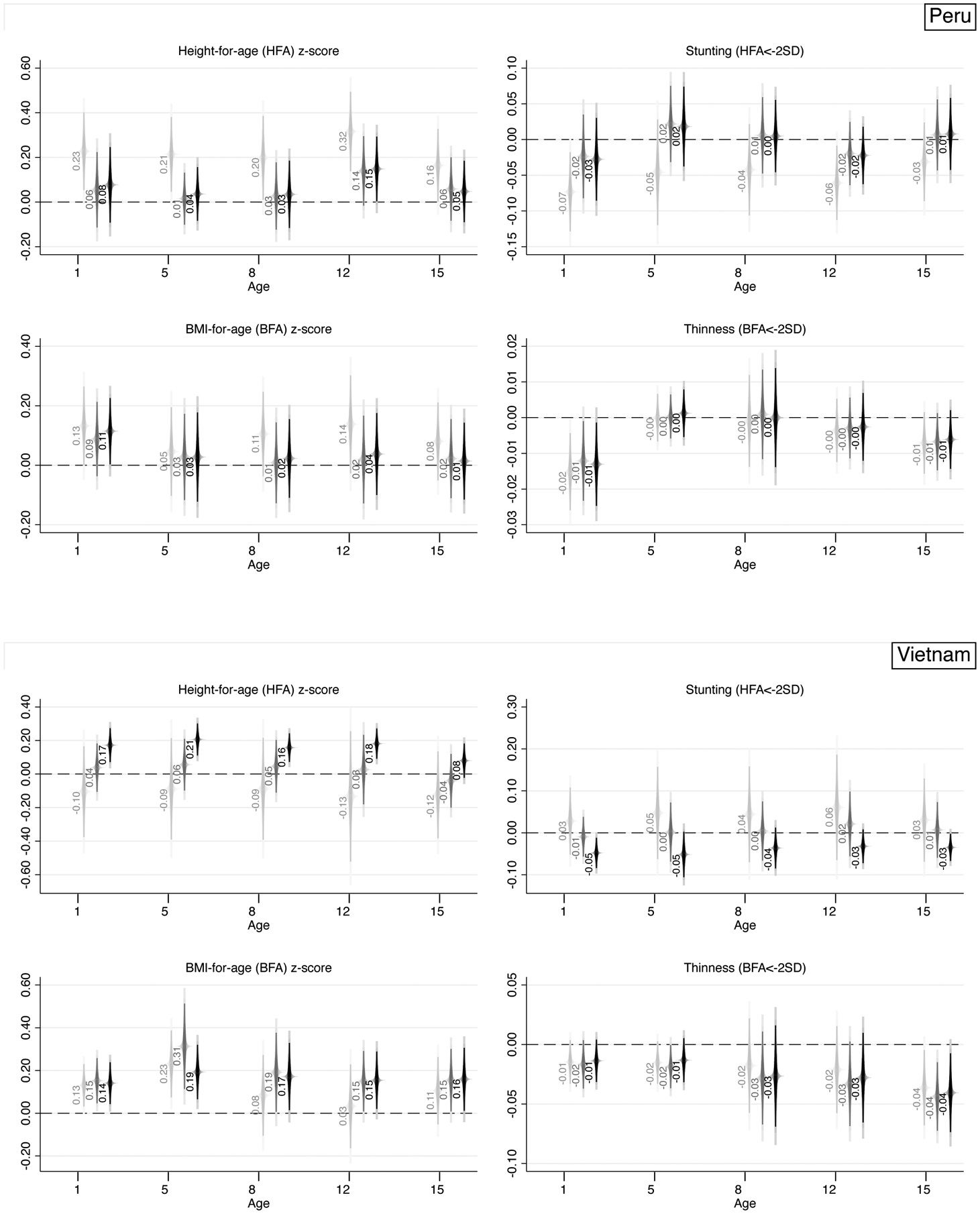
Association between parental educational similarity and children’s outcomes at different ages, by country – coefficient on homogamy reported, without controls (NC, light grey), controlling for maternal and paternal education (EDU, dark grey), and with full set of controls (FULL, black)

Notes: For each age, three coefficients on parental educational homogamy are reported: one with no controls (light grey, left), one with mother and father’s education as controls (dark grey, middle), and one with the full set of controls (black, right). 90, 95, and 99 percent (longest bars) confidence intervals reported.

Focusing exclusively on the sign of the estimated coefficients, results from Ethiopia suggest that parental educational similarity is associated with a lower HFA z-score and a higher probability of stunting, and lower BFA z-score and higher probability of thinness. The uncontrolled coefficients for HFA z-score and stunting are strong, stable in sign, and decreasing with age in terms of magnitude. Simply accounting for parents’ individual levels of education reduces the estimates by about a half and turns the estimates above age 5 non-significant. Differences between the NC and EDU specifications are starker relative to those between EDU and FULL, suggesting that individual levels of education account for a significant portion of the relationship between parental educational homogamy and children’s health – as hypothesized above. Nonetheless, results on HFA z-scores reveal that a negative association persists after accounting for the full set of controls at both ages 1 and 5. The HFA z-score of a child from an educationally-homogamous couple is lower by about 0.18–0.22 standard deviations (SD) relative to the HFA z-score of a child from an educationally-heterogamous couple. Results on BFA z-scores and thinness are fully in line in terms of sign (negative and positive, respectively), yet coefficients do not decrease in magnitude across ages and, if anything, they become more strongly significant in childhood (from age 8 onwards). For instance, in Ethiopia an 8-year-old child and a 15-year-old child from an educationally-homogamous couple have, respectively, a 4.6 and 5.3 percentage-point higher likelihood of being thin relative to a child from an educationally-heterogamous couple – corresponding to a 17 to 30 percent increase.

A similar pattern in terms of sign holds for India, where parental educational similarity is associated with a lower HFA z-score and a higher probability of stunting, and lower BFA z-score and higher probability of thinness. The uncontrolled coefficients for HFA z-score and stunting are strong, stable in sign, and decreasing with age in terms of magnitude – while estimated coefficients for BFA z-scores and thinness increase over age in absolute value. Accounting for parental education halves the size of the estimates, and additional controls further reduce their magnitudes. Full specifications in India suggest that a negative (positive) and statistically significant relationship between parental educational similarity and HFA z-scores (stunting) only persists at age 1. In India, a 1-year-old child from an educationally-homogamous couple has a 4.1 percentage-point higher likelihood of being stunted relative to a 1-year-old from an educationally-heterogamous couple – corresponding to a 17 percent increase.

A quick glance at Figure 3 is enough to realize that evidence from Peru and Vietnam is very different – almost specular with respect to Ethiopia and India – and more aligned with the few existing studies on the topic. Specifically, parental educational homogamy is positively associated with HFA z-scores and BFA z-scores, and negatively associated with stunting and thinness. Focusing on Peru, the signs of the coefficients are consistent with the pattern described above, yet the inclusion of controls makes most estimates non-significant. A few exceptions remain, such as BFA z-scores and thinness at age 1, where estimates suggest that a 1-year-old child from an educationally-homogamous couple in Peru has a 0.12 SD higher BFA z-score and a 1.3 percentage-point lower likelihood of being thin – corresponding to about a 50 percent decrease – relative to a child from an educationally-heterogamous couple. Estimated coefficients across ages are less consistent both in terms of magnitude and statistical significance.

Lastly, the case of Vietnam is unique for several reasons. First, the raw (NC) association between parental educational similarity and HFA z-scores is negative, while it turns positive when accounting for individual-level education of parents (EDU). The full specification provides strong and robust evidence that the association between parental educational similarity is positive and strongly statistically significant for HFA z-scores at least until age 8, with estimated coefficients quite stable in magnitude and varying between 0.16 and 0.21 SD. A similar observation can be made for stunting, with a negative and statistically significant association at age 1, 5, and 15. For instance, estimates at age 15 for stunting suggest that a child from an educationally-homogamous couple in Vietnam has a 3.5 percentage-point lower likelihood of being stunted – corresponding to about a 31.5 percent decrease – relative to a child from an educationally-heterogamous couple. Results supporting the homogamy-benefit hypothesis and its persistence across the early life-course are even stronger for BFA z-scores, with robust and statistically significant positive associations ranging from 0.14 to 0.19 SD up until age 15.

In sum, these findings depict a quite different reality across the four countries, with notable variation: (i) within countries across ages; (ii) within countries across outcomes, and (iii) between countries. For instance, (i) while in Vietnam the positive associations with z-scores are strong and stable across all ages (up until age 15), the same does not fully hold for their dichotomized counterparts (thinness, especially). Similarly, (ii) while in Ethiopia at age 1 there is a strong and negative statistically significant association between parental educational similarity and HFA z-scores, the same does not hold for BFA z-scores, where adding controls weakens the significance of the estimates. Lastly (iii), the sign of the estimates suggests that, for instance, homogamy is negatively associated with health outcomes in Ethiopia, while it is positively associated with health outcomes in Peru. In this latter respect, these analyses suggest the importance to focus on sign of the estimated coefficients and magnitudes, rather than statistical significance only (which is importantly affected by sample size and choice of controls). When focusing exclusively on signs, it is rather clear that findings from Figure 3 depict a different reality across two sets of countries. In the first one – Ethiopia and India – educational homogamy is negatively associated with children’s health; in the second one – Peru and Vietnam – educational homogamy is positively associated with children’s health, thus aligning more with the homogamy-benefit hypothesis. On top of this, it is possible to identify an additional source of within-group heterogeneity whereby in Ethiopia some negative associations seem to persist through adulthood (e.g., thinness at age 8 and 15), while in India they are mostly limited to infancy; similarly, in Vietnam the positive associations persist through adulthood for most analyzed outcomes, while in Peru they are limited to infancy. Appendix Figure A.1 provides the same set of estimates by country focusing on Weight-for-Age (WFA) z-scores and prevalence of underweight (two additional variables which combine characteristics of the variables included in the main analysis), confirming the negative associations in Ethiopia and India, alongside the positive associations in Peru and Vietnam.

Matching techniques

Table 5 provides estimates obtained through propensity score matching techniques and presents the Average Treatment Effect (ATE) associated to parental educational homogamy. Matching techniques complement OLS estimates as the former do not assume a priori any functional form for the relationship of interest, yet they still rely on the assumption that selection into educationally-homogamous couples is based on observable characteristics only – hence endogeneity may remain a source of concern.

Table 5:

Association between parental educational similarity and children’s health from non-parametric matching techniques, by country – Average Treatment Effect (ATE) reported

	Height-for-age (HFA)				BMI-for-age (BFA)
Ethiopia	HFA z-score		Stunting (<2SD)		BFA z-score		Thinness (<2SD)
	C(0.1)	NN(4)	C(0.1)	NN(4)	C(0.1)	NN(4)	C(0.1)	NN(4)
Age 1	−0.290**	−0.203*	0.066*	0.051*	−0.215*	−0.189*	0.057	0.070**
	(0.135)	(0.122)	(0.039)	(0.031)	(0.127)	(0.109)	(0.051)	(0.032)
Age 5	−0.181**	−0.130**	0.026	0.009	−0.051	−0.004	0.009	0.007
	(0.081)	(0.065)	(0.038)	(0.033)	(0.091)	(0.074)	(0.026)	(0.023)
Age 8	−0.123	−0.089	0.041	0.043	0.013	−0.014	0.018	0.003
	(0.081)	(0.071)	(0.035)	(0.027)	(0.095)	(0.098)	(0.040)	(0.039)
Age 12	−0.116	−0.066	0.036	0.000	−0.045	0.008	−0.001	−0.018
	(0.077)	(0.063)	(0.029)	(0.037)	(0.066)	(0.058)	(0.035)	(0.029)
Age 15	−0.039	−0.005	0.025	0.033	−0.091	−0.069	0.049	0.039
	(0.064)	(0.059)	(0.028)	(0.025)	(0.091)	(0.079)	(0.038)	(0.030)
	Height-for-age (HFA)				BMI-for-age (BFA)
India	HFA z-score		Stunting (<2SD)		BFA z-score		Thinness (<2SD)
	C(0.1)	NN(4)	C(0.1)	NN(4)	C(0.1)	NN(4)	C(0.1)	NN(4)
Age 1	−0.181*	−0.239**	0.071**	0.059*	0.063	0.001	−0.018	−0.006
	(0.110)	(0.099)	(0.033)	(0.030)	(0.092)	(0.075)	(0.028)	(0.022)
Age 5	−0.001	−0.007	−0.009	−0.020	0.046	0.064	−0.008	−0.012
	(0.080)	(0.064)	(0.038)	(0.033)	(0.073)	(0.064)	(0.027)	(0.026)
Age 8	−0.107	−0.025	−0.002	0.009	0.051	0.060	−0.007	−0.019
	(0.090)	(0.080)	(0.033)	(0.030)	(0.105)	(0.088)	(0.033)	(0.027)
Age 12	−0.008	0.019	−0.017	−0.019	−0.078	−0.141	0.030	0.032
	(0.075)	(0.070)	(0.038)	(0.033)	(0.101)	(0.090)	(0.031)	(0.027)
Age 15	−0.013	0.000	0.001	0.000	−0.058	−0.054	0.045	0.037
	(0.079)	(0.068)	(0.032)	(0.030)	(0.103)	(0.086)	(0.030)	(0.026)
	Height-for-age (HFA)				BMI-for-age (BFA)
Peru	HFA z-score		Stunting (<2SD)		BFA z-score		Thinness (<2SD)
	C(0.1)	NN(4)	C(0.1)	NN(4)	C(0.1)	NN(4)	C(0.1)	NN(4)
Age 1	0.050	0.015	−0.020	−0.008	0.086	0.095	−0.018***	−0.016***
	(0.121)	(0.103)	(0.038)	(0.031)	(0.109)	(0.089)	(0.006)	(0.006)
Age 5	0.024	0.042	−0.041	−0.018	0.025	0.003	−0.001	−0.002
	(0.084)	(0.078)	(0.047)	(0.038)	(0.092)	(0.078)	(0.002)	(0.003)
Age 8	0.011	0.017	−0.036	−0.018	0.043	0.005	−0.012	−0.003
	(0.078)	(0.072)	(0.035)	(0.026)	(0.078)	(0.069)	(0.010)	(0.008)
Age 12	0.111	0.118	−0.010	−0.020	0.034	0.030	−0.007	−0.005
	(0.088)	(0.083)	(0.029)	(0.029)	(0.074)	(0.068)	(0.006)	(0.004)
Age 15	0.076	0.069	−0.037	−0.030	0.068	0.040	−0.006	−0.008
	(0.065)	(0.059)	(0.028)	(0.020)	(0.067)	(0.066)	(0.005)	(0.006)
	Height-for-age (HFA)				BMI-for-age (BFA)
Vietnam	HFA z-score		Stunting (<2SD)		BFA z-score		Thinness (<2SD)
	C(0.1)	NN(4)	C(0.1)	NN(4)	C(0.1)	NN(4)	C(0.1)	NN(4)
Age 1	0.211***	0.152**	−0.072***	−0.038*	0.126*	0.102*	−0.005	−0.022*
	(0.071)	(0.066)	(0.019)	(0.021)	(0.067)	(0.058)	(0.011)	(0.012)
Age 5	0.205***	0.201***	−0.051**	−0.047**	0.140**	0.209***	−0.013	−0.012
	(0.065)	(0.054)	(0.022)	(0.020)	(0.062)	(0.059)	(0.010)	(0.009)
Age 8	0.189**	0.130**	−0.041	−0.024	0.142*	0.180***	−0.021	−0.031**
	(0.074)	(0.054)	(0.031)	(0.023)	(0.085)	(0.069)	(0.017)	(0.015)
Age 12	0.096	0.140**	0.007	−0.008	0.161**	0.209***	−0.033*	−0.038**
	(0.066)	(0.056)	(0.020)	(0.020)	(0.082)	(0.065)	(0.019)	(0.016)
Age 15	0.104	0.058	−0.031	−0.021	0.201**	0.153**	−0.048*	−0.043**
	(0.063)	(0.051)	(0.027)	(0.019)	(0.086)	(0.067)	(0.028)	(0.019)

Notes:

^***:p<0.01;

^**:p<0.05;

^*p<0.1.

C(0,1): Caliper 0.1; NN(4): nearest-neighbor matching with 4 matches per observation.

Table 5 delivers a clear set of findings. In Ethiopia and India, most of the negative associations between educational homogamy and children’s outcomes observed in the previous section persist, yet they are confined to the very early ages (age 1 and, to a lesser extent, age 5). In Ethiopia, a child from an educationally-homogamous couple has a probability of being stunted at age 1 that is 5–7 percentage-points higher than that of a child from an educationally-heterogamous one – corresponding to a 14–19 percent increase. This same estimate is 6–7 percentage points in India (close to the 7–12 percentage-point estimate obtained through OLS) – corresponding to a 24–29 percent increase. For Ethiopia, the statistically significant positive associations between homogamy and thinness observed at some older ages disappear when using matching techniques. Overall, there is no more evidence of negative associations between parental educational similarity and children’s health in childhood and adulthood in either country.

As for Peru and Vietnam, the positive associations documented with OLS persist, yet in Peru the statistical significance largely disappears – except for BMI-for-age at age 1 (thinness). These matching estimates for Peru suggest that a child from an educationally-homogamous couple has a probability of being thin at age 1 that is 1.6–1.8 percentage-point lower than a child from an educationally-heterogamous couple. Vietnam turns out to be the most interesting case study, as it is the only country where the positive associations remain strong and statistically significant in infancy, childhood, and early adolescence. These positive associations can be observed across all outcomes, yet more neatly for the HFA and BFA continuous scores. Evidence for Vietnam from both OLS and matching techniques is therefore fully supportive of a homogamy-benefit hypothesis which persists all the way through early adulthood.

Ancillary analyses

Birth-related outcomes

To better situate this study within the literature – which mainly focuses on children’s health at birth – I provide some estimates predicting birth-related outcomes, namely birth weight, low-birth weight (dummy=1 if the weight of the child is lower than 2,500 grams), probability of breastfeeding, probability of having any antenatal visit during pregnancy, number of antenatal visits, whether the child was delivered by a skilled professional, and whether the child received vaccinations for measles and BCG. These outcomes were not made the central focus of the study as the variables contain high missing information.

Results on these outcomes – reported in Table A.4 – provide mixed evidence, likely due to the incompleteness of birth-related data. In Peru and Vietnam few associations are statistically significant. As for Ethiopia and India, results support the idea from the above sections that – if anything – parental educational homogamy is associated with worse health outcomes of children. Specifically, parental educational homogamy is associated with a lower probability of scheduling antenatal visits, a lower actual number of antenatal visits, and lower likelihood of delivery by a skilled professional. Due to small sample sizes, associations with birth weight are not statistically significant yet the estimated coefficient is negative in Ethiopia and India, and positive in Peru and Vietnam, in line with the above.

Education in categories

I then test the sensitivity of the results to an alternative definition of parental educational homogamy obtained through the education variable coded categorically rather than continuously. As India and Peru are the two countries in which the share of educationally-homogamous couples differs the most across definitions (Table 3), I run the same OLS estimates presented in Figure 3 only for these two countries. Results – reported in Table A.5 – are qualitatively the same for both countries in terms of patterns over age, across outcomes, and magnitude of the coefficients. In terms of magnitude, estimates for India are slightly smaller (e.g., −0.161 for HFA z-score at age 1 in the previous specification against −0.128 in the current one). Uncontrolled estimates for Peru are slightly bigger, yet estimates accounting for controls are very much in line (e.g., 0.115 for BFA z-score at age 1 in the previous specification against 0.117 in the current one).

Bounds for “missing” couples

I next evaluate whether “missing” couples, i.e. those for which parental educational similarity cannot be obtained due to missing father’s information, are responsible for driving the observed associations. As the share of missing data is higher than 5 percent only in Ethiopia and Peru, I limit the sensitivity tests to these two countries. Specifically, I bound the estimates assuming first all missing fathers to have the same level of education as the mother (H1: all missing couples, if present, would be educationally homogamous), and then to have a different level of education from the mother (H2: all missing couples, if present, would be educationally heterogamous). Results from OLS for Ethiopia – presented in Table A.6 – are very consistent regardless of scenario. For Peru, results are strong and robust under H2, while they depart more under H1, as HFA coefficients lose statistical significance. BFA coefficients are more stable irrespective of scenario. For instance, regardless of H1 or H2, a child from an educationally-homogamous couple in Peru has a 1.3 percentage-point lower likelihood of being thin relative to a child from an educationally-heterogamous couple. As educational homogamy is far less prevalent in Peru than in other countries (Table 3), discrepancies observed under H1 are unlikely to be problematic as it would be rather implausible to expect all missing couples in Peru to be educationally homogamous. If anything, it might be more reasonable to expect missing couples to be educationally heterogamous.

Educational upgrading

Lastly, I rerun estimates only keeping mothers ages 25 and above in wave 1 to deal with possible concerns of educational upgrading whereby younger mothers might still be in education at a younger age. Arguably, this sample gives a more accurate picture of parental educational homogamy. OLS estimates – presented in Table A.7 – are fully consistent with the ones reported in Figure 3. Overall, coefficients are bigger in magnitude and more strongly statistically significant. Patterns over age and across outcomes are unaltered.

Conclusions and discussion

In this study I have explored the relationship between parental educational similarity and children’s health outcomes in geographically selected areas of four low- and middle-income countries, focusing on children’s outcomes longitudinally from birth to middle adolescence (age 15). I have explored a range of health outcomes, namely height-for-age (HFA) and BMI-for-age (BFA) z-scores, alongside their dichotomized counterparts stunting and thinness, and conducted analyses in Ethiopia, India, Peru, and Vietnam using a combination of OLS and non-parametric matching techniques. Using OLS and accounting for a wide set of controls, I have found that in Ethiopia and India parental educational homogamy is associated with worse health outcomes in both infancy and childhood, while associations are positive in Peru and Vietnam. Estimates from matching techniques provide consistent results in terms of direction of the association (sign), yet they suggest that these associations fade after age 1, except in Vietnam, where the positive and significant relationship persists through adolescence.

Focusing on Peru and Vietnam, my findings align with family systems theory and the homogamy-benefit hypothesis whereby parental educational similarity is beneficial for children’s outcomes due to enhanced complementarity in parental inputs towards child production, relationship quality, and reduced conflict and stress in both the prenatal and postnatal period. The fading of these positive associations in Peru after age 1 suggests that the mechanisms might act primarily in the prenatal and immediate postnatal period and might have to do mostly with reductions in maternal stress and anxiety which does not carry forward in children’s lives. Evidence suggests that prenatal stress accounts for approximately 10 percent of the variation in multiple infant health measures (Beijers et al. 2010). In this context, parental educational similarity might translate into greater agreement on perinatal decisions such as medical screenings or breastfeeding practices. Conversely, the robust positive associations observed in Vietnam in infancy, childhood, and early adolescence would seem to suggest that – on top of reductions in maternal stress during pregnancy which are carried forward during the life course – other long-lasting postnatal mechanisms might be at play such as complementarity in parental inputs at multiple life stages of the child (e.g., parental agreement on schooling decisions), more equitable sharing of childrearing responsibilities, and enhanced relationship quality and stability as reflected, for instance, into lower likelihood of marital dissolution. In reference to the literature, findings from Peru and Vietnam align with the existing limited evidence from upper middle- and high-income societies (Abufhele et al. 2020; Rauscher 2020), which I had also reformulated myself in the background section.

Conversely, evidence from Ethiopia and India runs largely against the homogamy-benefit hypothesis, a finding which is rather new in the literature and suggests the existence of important heterogeneity in the relationship across countries at different levels of development and with different socio-economic characteristics, societal customs, family traditions, and gender dynamics. Although several explanations could lie behind this negative association, the most likely is that in societies where status inconsistencies between men and women are the norm, status homogamy would actually bring disruptions to daily life and be associated with higher levels of stress and tension (Cools & Kotsadam, 2017), thus “neutralizing” and even reverting the potential beneficial effects of educational homogamy. Relatedly, it might be the case that given the poor quality of education and the low returns to schooling in some sub-Saharan countries such as Ethiopia, improvements in mother’s educational status might do little to change her bargaining power (Behrman 2019). The finding that these negative associations fade after age 1 is particularly relevant (and relatively “good news”) in contexts such as Ethiopia and India that are experiencing important educational expansion and increasing educational attainment, particularly on the part of women – which will in turn make educationally-homogamous couples an even more prevalent couple configuration.

Although tested only indirectly here, the evidence from these four countries combined seem to suggest that the level of a country’s development, the extent of gender equality that exists within a society and within couples, the specific family practices that prevail (e.g., arranged marriage), and the aggregate levels of education of men and women matter for the strength and direction of the association. This study only focuses on four countries, yet based on these findings it would be reasonable to speculate the existence of a continuum and a specific threshold of a combined “education-family-gender and development index” for low- and middle-income countries whereby the within-country associations between parental educational similarity and children’s outcomes are negative if countries rank below this threshold (Ethiopia and India here) and positive if countries rank above this threshold (Peru and Vietnam here). In line with this speculation, I will pick up on this idea and test it empirically in subsequent research using nationally representative data from multiple countries (80+) from, for instance, the Demographic and Health Surveys.

This study has some limitations that lay the ground for subsequent research. First, due to the YL sampling design, the prevalence figures presented in this paper are not in line with country-level statistics on the prevalence of parental educational homogamy and children’s anthropometric outcomes. The evidence provided here is limited to geographically selected areas in the four countries, as the YL design purposively oversamples poor areas. For reference, Table A.8 provides a comparison of YL and DHS estimates on parental educational homogamy and children’s anthropometric outcomes, suggesting that these discrepancies need to be kept in mind when thinking about generalizability of results.⁷ Second, and most importantly, the evidence provided remains associational. Even though I include a wide array of controls and complement OLS estimates with matching techniques, the latter strategy does not allow to overcome the issue of selection on unobservables. As such, although reverse causality is not a concern in this setting, endogeneity due to omitted variable bias and selection on unobservables still is. Alternative strategies relying on potential sources of exogenous variation should be considered to minimize this bias, yet these are hard to implement in cross-country comparative studies of this kind. Country-specific studies might be better suited to address this specific concern.

Despite the above limitations, this analysis is – to the best of my knowledge – unique in its attempt to bring the study of the intergenerational implications of parental educational assortative mating to a cross-country context. As such, it provides an initial overview of how this relationship changes over a child’s life-course – very little in three out of the four countries considered – and how much it varies across four diverse low-income settings that are currently experiencing important processes of educational expansion. Future research should capitalize on this study and bring the analysis of this relationship to a truly global and comparative scale using pooled nationally representative surveys.

Appendix Tables

Table A.1:

Correlations between anthropometric outcomes, by age of the child (wave), pooled sample.

Age 1	HFA z-score	BFA z-score	WFA z-score
HFA z-score	1.000	.	.
BFA z-score	−0.080	1.000	.
WFA z-score	0.640	0.712	1.000
Age 5	HFA z-score	BFA z-score	WFA z-score
HFA z-score	1.000	.	.
BFA z-score	−0.075	1.000	.
WFA z-score	0.634	0.720	1.000
Age 8	HFA z-score	BFA z-score	WFA z-score
HFA z-score	1.000	.	.
BFA z-score	0.056	1.000	.
WFA z-score	0.641	0.796	1.000
Age 12	HFA z-score	BFA z-score	WFA z-score
HFA z-score	1.000	.	.
BFA z-score	0.278	1.000	.
WFA z-score	.	.	.
Age 15	HFA z-score	BFA z-score	WFA z-score
HFA z-score	1.000	.	.
BFA z-score	0.188	1.000	.
WFA z-score	.	.	.

Table A.2:

Attrition analysis; t-tests for differences in means between children present in all rounds and children who left the study in any round following the first

	Ethiopia			India
	Present in all rounds	Attrition after R1 (9.8%)	Diff.	Present in all rounds	Attrition after R1 (6%)	Diff.
Child is female (Ref.: Male)	0.470	0.526	−0.056	0.462	0.475	−0.013
			(0.038)			(0.047)
Age of the child (months)	11.67	11.65	0.021	11.83	11.68	0.157
			(0.268)			(0.329)
Mother’s grade attained	2.324	3.037	−0.713***	2.959	3.368	−0.410
			(0.276)			(0.405)
Father’s grade attained	3.026	3.691	−0.664*	4.427	4.652	−0.225
			(0.363)			(0.472)
Number of siblings	2.189	1.958	−0.231	0.710	0.700	0.010
			(0.150)			(0.096)
Household size	5.765	5.327	0.439***	5.446	5.042	0.404
			(0.162)			(0.282)
Household is in urban area (Ref.: Rural)	0.339	0.454	−0.115***	0.238	0.475	−0.236***
			(0.036)			(0.041)
HFA z-score	−1.536	−1.741	0.205	−1.333	−1.406	0.072
			(0.130)			(0.152)
BFA z-score	−0.669	−0.819	0.150	−1.034	−1.099	0.064
			(0.122)			(0.111)
	Peru			Vietnam
	Present in all rounds	Attrition after R1 (11.9%)	Diff.	Present in all rounds	Attrition after R1 (5.4%)	Diff.
Child is female (Ref.: Male)	0.496	0.527	−0.031	0.488	0.468	0.020
			(0.034)			(0.049)
Age of the child (months)	11.54	11.48	0.067	11.65	11.10	0.554*
			(0.241)			(0.311)
Mother’s grade attained	7.140	7.191	−0.050	5.523	6.691	−1.168***
			(0.344)			(0.439)
Father’s grade attained	8.258	8.445	−0.187	6.081	7.456	−1.375***
			(0.358)			(0.451)
Number of siblings	1.312	1.269	0.042	0.829	0.725	0.104
			(0.112)			(0.101)
Household size	5.710	5.661	0.049	4.902	4.862	0.039
			(0.159)			(0.181)
Household is in urban area (Ref.: Rural)	0.682	0.710	−0.028	0.183	0.495	−0.312***
			(0.032)			(0.039)
HFA z-score	−1.279	−1.421	0.142	−1.126	−0.961	−0.165
			(0.092)			(0.132)
BFA z-score	0.787	0.828	−0.042	−0.410	−0.356	−0.054
			(0.089)			(0.097)

Notes:

^***p<0.01,

^**p<0.05,

^*p<0.1

Table A.3:

Association between parental educational homogamy and children’s outcomes at different ages, by country

	Height-for-age (HFA)						BMI-for-age (BFA)
Ethiopia	HFA z- score			Stunting (<−2SD)			BFA z- score			Thinness (<−2SD)
	NC	EDU	FULL	NC	EDU	FULL	NC	EDU	FULL	NC	EDU	FULL
Age 1	−0.351**	−0.180*	−0.220**	0.088***	0.011	0.012	−0.390*	−0.058	0.018	0.042	−0.010	−0.025
	(0.143)	(0.099)	(0.083)	(0.029)	(0.024)	(0.016)	(0.198)	(0.137)	(0.109)	(0.043)	(0.031)	(0.024)
Age 5	−0.338***	−0.138	−0.180**	0.082**	0.012	0.033	−0.094	−0.061	0.056	0.012	0.020	0.003
	(0.093)	(0.093)	(0.067)	(0.029)	(0.037)	(0.032)	(0.089)	(0.097)	(0.079)	(0.012)	(0.018)	(0.018)
Age 8	−0.279***	−0.099	−0.092	0.077***	0.036	0.036*	−0.230**	−0.120	−0.061	0.089**	0.062**	0.046*
	(0.088)	(0.080)	(0.067)	(0.025)	(0.025)	(0.021)	(0.099)	(0.076)	(0.066)	(0.031)	(0.025)	(0.024)
Age 12	−0.277***	−0.126	−0.076	0.103***	0.037	0.019	−0.239**	−0.054	−0.019	0.104**	0.068*	0.046
	(0.082)	(0.084)	(0.079)	(0.030)	(0.036)	(0.036)	(0.089)	(0.070)	(0.056)	(0.042)	(0.037)	(0.034)
Age 15	−0.235**	−0.073	−0.053	0.083***	0.022	0.015	−0.334***	−0.162**	−0.101	0.123***	0.078**	0.053*
	(0.087)	(0.076)	(0.054)	(0.028)	(0.024)	(0.018)	(0.104)	(0.075)	(0.060)	(0.035)	(0.029)	(0.025)
	Height-for-age (HFA)						BMI-for-age (BFA)
India	HFA z- score			Stunting (<−2SD)			BFA z- score			Thinness (<−2SD)
	NC	EDU	FULL	NC	EDU	FULL	NC	EDU	FULL	NC	EDU	FULL
Age 1	−0.436***	−0.223**	−0.161*	0.127***	0.053**	0.041*	−0.110*	0.070	0.051	−0.002	−0.045*	−0.040
	(0.069)	(0.080)	(0.088)	(0.022)	(0.020)	(0.023)	(0.060)	(0.061)	(0.049)	(0.025)	(0.025)	(0.024)
Age 5	−0.279***	−0.004	−0.003	0.089**	−0.010	−0.011	0.007	0.051	0.059	−0.018	−0.017	−0.017
	(0.064)	(0.070)	(0.073)	(0.034)	(0.035)	(0.037)	(0.052)	(0.064)	(0.060)	(0.027)	(0.031)	(0.032)
Age 8	−0.264***	0.044	0.035	0.104***	0.020	0.011	−0.177**	0.027	0.056	0.036	−0.015	−0.019
	(0.063)	(0.064)	(0.069)	(0.029)	(0.030)	(0.031)	(0.070)	(0.090)	(0.085)	(0.024)	(0.028)	(0.029)
Age 12	−0.282***	0.026	0.036	0.073**	−0.013	−0.022	−0.423***	−0.078	−0.041	0.087***	0.018	0.010
	(0.070)	(0.078)	(0.084)	(0.030)	(0.030)	(0.033)	(0.059)	(0.082)	(0.079)	(0.020)	(0.027)	(0.025)
Age 15	−0.176***	0.022	0.033	0.066**	0.000	−0.011	−0.334***	−0.089	−0.042	0.068***	0.031	0.013
	(0.056)	(0.068)	(0.065)	(0.024)	(0.029)	(0.030)	(0.051)	(0.060)	(0.065)	(0.017)	(0.023)	(0.023)
	Height-for-age (HFA)						BMI-for-age (BFA)
Peru	HFA z- score			Stunting (<−2SD)			BFA z- score			Thinness (<−2SD)
	NC	EDU	FULL	NC	EDU	FULL	NC	EDU	FULL	NC	EDU	FULL
Age 1	0.228**	0.055	0.077	−0.073**	−0.024	−0.028	0.132**	0.088	0.115**	−0.015**	−0.012**	−0.013**
	(0.083)	(0.081)	(0.081)	(0.027)	(0.028)	(0.028)	(0.063)	(0.060)	(0.053)	(0.005)	(0.005)	(0.006)
Age 5	0.214**	0.015	0.036	−0.046	0.022	0.018	0.046	0.028	0.028	−0.000	0.000	0.001
	(0.080)	(0.056)	(0.057)	(0.035)	(0.025)	(0.027)	(0.071)	(0.069)	(0.071)	(0.003)	(0.003)	(0.003)
Age 8	0.198**	0.027	0.035	−0.042	0.006	0.005	0.105	0.008	0.023	−0.001	0.001	0.000
	(0.090)	(0.072)	(0.072)	(0.031)	(0.026)	(0.024)	(0.068)	(0.065)	(0.063)	(0.006)	(0.006)	(0.007)
Age 12	0.316***	0.139*	0.148**	−0.061**	−0.020	−0.022	0.138*	0.019	0.038	−0.004	−0.003	−0.003
	(0.085)	(0.074)	(0.069)	(0.025)	(0.021)	(0.019)	(0.079)	(0.070)	(0.066)	(0.004)	(0.004)	(0.005)
Age 15	0.164**	0.058	0.047	−0.031	0.007	0.008	0.080	0.022	0.014	−0.007	−0.007*	−0.006
	(0.078)	(0.068)	(0.066)	(0.026)	(0.024)	(0.024)	(0.063)	(0.064)	(0.062)	(0.004)	(0.004)	(0.004)
	Height-for-age (HFA)						BMI-for-age (BFA)
Vietnam	HFA z- score			Stunting (<−2SD)			BFA z- score			Thinness (<−2SD)
	NC	EDU	FULL	NC	EDU	FULL	NC	EDU	FULL	NC	EDU	FULL
Age 1	−0.105	0.038	0.172***	0.028	−0.009	−0.048**	0.131**	0.152***	0.141***	−0.015	−0.017	−0.014
	(0.129)	(0.069)	(0.048)	(0.038)	(0.023)	(0.017)	(0.047)	(0.050)	(0.047)	(0.009)	(0.010)	(0.008)
Age 5	−0.088	0.056	0.206***	0.047	0.002	−0.052*	0.231**	0.313***	0.193***	−0.015*	−0.019**	−0.013
	(0.145)	(0.074)	(0.046)	(0.053)	(0.034)	(0.026)	(0.075)	(0.096)	(0.061)	(0.009)	(0.009)	(0.009)
Age 8	−0.088	0.046	0.158***	0.044	0.004	−0.036	0.083	0.192**	0.172**	−0.018	−0.028	−0.027
	(0.146)	(0.075)	(0.041)	(0.055)	(0.034)	(0.023)	(0.091)	(0.089)	(0.075)	(0.019)	(0.019)	(0.020)
Age 12	−0.134	0.026	0.181***	0.060	0.021	−0.032	0.032	0.150**	0.154**	−0.021	−0.033*	−0.028
	(0.186)	(0.099)	(0.043)	(0.060)	(0.037)	(0.019)	(0.094)	(0.068)	(0.064)	(0.018)	(0.017)	(0.018)
Age 15	−0.124	−0.041	0.080	0.030	0.007	−0.035**	0.105	0.155**	0.159**	−0.036**	−0.044***	−0.041**
	(0.124)	(0.077)	(0.049)	(0.047)	(0.032)	(0.016)	(0.076)	(0.070)	(0.070)	(0.015)	(0.014)	(0.016)

Notes: NC: no controls; EDU: controls for mother and father’s education; FULL: all controls. Only educational homogamy coefficient reported. Robust standard errors in parentheses.

^***p<0.01,

^**p<0.05,

^*p<0.1

Table A.4:

Association between parental educational homogamy and children’s birth-related outcomes, by country

Birth-related outcomes	Ethiopia		India		Peru		Vietnam
	NC	FULL	NC	FULL	NC	FULL	NC	FULL
Birth weight (grams)	−171.893	−29.194	−17.466	−47.341	35.321	−0.906	31.330	36.207
	(226.715)	(112.399)	(32.320)	(35.464)	(30.923)	(28.865)	(26.938)	(26.335)
Low birth weight (<2500 grams)	0.067	0.006	−0.018	−0.024	0.023	0.027	−0.001	−0.001
	(0.044)	(0.033)	(0.019)	(0.018)	(0.016)	(0.016)	(0.013)	(0.014)
Ever breastfed (Ref.: No)	0.008	−0.013	0.003	0.002	−0.011*	−0.010	0.001	0.002
	(0.008)	(0.010)	(0.008)	(0.010)	(0.006)	(0.006)	(0.004)	(0.004)
Any antenatal visits during pregnancy (Ref. : No)	−0.156***	−0.040	−0.053**	−0.033*	−0.011	−0.019	−0.106	−0.008
	(0.052)	(0.027)	(0.025)	(0.019)	(0.013)	(0.013)	(0.072)	(0.011)
Number of antenatal visits	−0.999***	−0.165	−0.784***	−0.201	0.326	0.049	−0.273	0.112
	(0.340)	(0.148)	(0.171)	(0.154)	(0.210)	(0.191)	(0.259)	(0.069)
Delivery skilled professional (Ref.: No)	−0.135**	0.030	−0.159***	0.006	0.026	−0.028	−0.174*	−0.041**
	(0.051)	(0.026)	(0.032)	(0.025)	(0.026)	(0.017)	(0.096)	(0.018)
Measles: Child has received vaccination (Ref.: No)	0.026	0.046*	−0.048	−0.030	−0.000	−0.002	−0.054*	−0.023
	(0.040)	(0.026)	(0.031)	(0.026)	(0.031)	(0.036)	(0.026)	(0.023)
BCG: Child has received vaccination (Ref.: No)	−0.033	−0.019	−0.012	−0.010	0.006	0.004	−0.015	0.020
	(0.037)	(0.023)	(0.013)	(0.015)	(0.008)	(0.009)	(0.020)	(0.014)

Notes: NC: no controls; FULL: all controls. Only educational homogamy coefficient reported. Robust standard errors in parentheses.

^***p<0.01,

^**p<0.05,

^*p<0.1

Table A.5:

Association between parental educational homogamy computed through categorical variables and children’s outcomes at different ages, for India and Peru

	Height-for-age (HFA)				BMI-for-age (BFA)
India	HFA z-score		Stunting (<−2SD)		BFA z-score		Thinness (<−2SD)
	NC	FULL	NC	FULL	NC	FULL	NC	FULL
Age 1	−0.381***	−0.128*	0.109***	0.032	−0.108*	0.013	0.001	−0.025
	(0.072)	(0.069)	(0.022)	(0.024)	(0.053)	(0.046)	(0.023)	(0.021)
Age 5	−0.255***	−0.030	0.081**	0.001	0.013	0.048	−0.018	−0.018
	(0.065)	(0.063)	(0.034)	(0.035)	(0.044)	(0.059)	(0.024)	(0.026)
Age 8	−0.218***	0.021	0.081***	0.003	−0.117	0.090	0.018	−0.035
	(0.060)	(0.057)	(0.029)	(0.027)	(0.072)	(0.079)	(0.025)	(0.028)
Age 12	−0.258***	−0.006	0.055*	−0.024	−0.261***	0.118	0.067***	−0.006
	(0.066)	(0.086)	(0.029)	(0.030)	(0.084)	(0.101)	(0.020)	(0.018)
Age 15	−0.185***	−0.032	0.056**	−0.008	−0.265***	0.008	0.055***	0.004
	(0.053)	(0.058)	(0.022)	(0.023)	(0.058)	(0.066)	(0.017)	(0.021)
	Height-for-age (HFA)				BMI-for-age (BFA)
Peru	HFA z-score		Stunting (<−2SD)		BFA z-score		Thinness (<−2SD)
	NC	FULL	NC	FULL	NC	FULL	NC	FULL
Age 1	0.377***	0.022	−0.112***	−0.005	0.200***	0.117*	−0.012*	−0.009
	(0.084)	(0.082)	(0.030)	(0.031)	(0.064)	(0.066)	(0.007)	(0.009)
Age 5	0.426***	0.022	−0.123***	0.023	0.118	0.087	−0.001	−0.001
	(0.083)	(0.070)	(0.034)	(0.032)	(0.074)	(0.076)	(0.003)	(0.003)
Age 8	0.381***	0.019	−0.085***	0.020	0.239***	0.074	0.000	0.001
	(0.079)	(0.065)	(0.028)	(0.025)	(0.083)	(0.072)	(0.005)	(0.005)
Age 12	0.439***	0.074	−0.081***	0.004	0.261***	0.057	−0.004	−0.003
	(0.075)	(0.060)	(0.025)	(0.020)	(0.080)	(0.063)	(0.005)	(0.005)
Age 15	0.243***	0.005	−0.057**	0.019	0.084	−0.024	−0.001	−0.003
	(0.072)	(0.063)	(0.027)	(0.025)	(0.056)	(0.053)	(0.004)	(0.005)

Notes: NC: no controls; FULL: all controls. Only homogamy coefficient reported. Robust standard errors in parentheses.

^***p<0.01,

^**p<0.05,

^*p<0.1

Table A.6:

Bounded estimates assuming all missing couples to be homogamous (H1) and all missing couples to be heterogamous (H2), for Ethiopia and Peru

H1: All missing couples are homogamous
	Height-for-age (HFA)				BMI-for-age (BFA)
Ethiopia	HFA z-score		Stunting (<−2SD)		BFA z-score		Thinness (<−2SD)
	NC	FULL	NC	FULL	NC	FULL	NC	FULL
Age 1	−0.343**	−0.220**	0.089***	0.012	−0.321*	0.018	0.038	−0.025
	(0.122)	(0.083)	(0.026)	(0.016)	(0.166)	(0.109)	(0.036)	(0.024)
Age 5	−0.292***	−0.180**	0.072**	0.033	−0.130	0.056	0.013	0.003
	(0.083)	(0.067)	(0.027)	(0.032)	(0.081)	(0.079)	(0.011)	(0.018)
Age 8	−0.241***	−0.092	0.070***	0.036*	−0.220**	−0.061	0.090***	0.046*
	(0.077)	(0.067)	(0.023)	(0.021)	(0.084)	(0.066)	(0.026)	(0.024)
Age 12	−0.228***	−0.076	0.092***	0.019	−0.219**	−0.019	0.102**	0.046
	(0.075)	(0.079)	(0.027)	(0.036)	(0.077)	(0.056)	(0.038)	(0.034)
Age 15	−0.186**	−0.053	0.067**	0.015	−0.285***	−0.101	0.099***	0.053*
	(0.076)	(0.054)	(0.024)	(0.018)	(0.085)	(0.060)	(0.029)	(0.025)
	Height-for-age (HFA)				BMI-for-age (BFA)
Peru	HFA z-score		Stunting (<−2SD)		BFA z-score		Thinness (<−2SD)
	NC	FULL	NC	FULL	NC	FULL	NC	FULL
Age 1	0.141	0.077	−0.038	−0.028	0.082	0.115**	−0.009*	−0.013**
	(0.085)	(0.081)	(0.022)	(0.028)	(0.060)	(0.053)	(0.005)	(0.006)
Age 5	0.090	0.036	−0.014	0.018	0.032	0.028	0.005	0.001
	(0.076)	(0.057)	(0.029)	(0.027)	(0.072)	(0.071)	(0.004)	(0.003)
Age 8	0.078	0.035	−0.021	0.005	0.052	0.023	0.000	0.000
	(0.082)	(0.072)	(0.027)	(0.024)	(0.065)	(0.063)	(0.005)	(0.007)
Age 12	0.171**	0.148**	−0.030	−0.022	0.087	0.038	0.002	−0.003
	(0.076)	(0.069)	(0.021)	(0.019)	(0.059)	(0.066)	(0.004)	(0.005)
Age 15	0.046	0.047	−0.010	0.008	0.042	0.014	−0.005	−0.006
	(0.066)	(0.066)	(0.022)	(0.024)	(0.058)	(0.062)	(0.004)	(0.004)
H2: All missing couples are heterogamous
	Height-for-age (HFA)				BMI-for-age (BFA)
Ethiopia	HFA z-score		Stunting (<−2SD)		BFA z-score		Thinness (<−2SD)
	NC	FULL	NC	FULL	NC	FULL	NC	FULL
Age 1	−0.270*	−0.220**	0.064**	0.012	−0.373*	0.018	0.037	−0.025
	(0.141)	(0.083)	(0.030)	(0.016)	(0.197)	(0.109)	(0.042)	(0.024)
Age 5	−0.308***	−0.180**	0.074**	0.033	−0.026	0.056	0.008	0.003
	(0.090)	(0.067)	(0.028)	(0.032)	(0.077)	(0.079)	(0.011)	(0.018)
Age 8	−0.256***	−0.092	0.067**	0.036*	−0.183*	−0.061	0.064*	0.046*
	(0.089)	(0.067)	(0.025)	(0.021)	(0.097)	(0.066)	(0.031)	(0.024)
Age 12	−0.268***	−0.076	0.090***	0.019	−0.203**	−0.019	0.080**	0.046
	(0.074)	(0.079)	(0.028)	(0.036)	(0.082)	(0.056)	(0.036)	(0.034)
Age 15	−0.236***	−0.053	0.082***	0.015	−0.309***	−0.101	0.120***	0.053*
	(0.080)	(0.054)	(0.026)	(0.018)	(0.103)	(0.060)	(0.036)	(0.025)
	Height-for-age (HFA)				BMI-for-age (BFA)
Peru	HFA z-score		Stunting (<−2SD)		BFA z-score		Thinness (<−2SD)
	NC	FULL	NC	FULL	NC	FULL	NC	FULL
Age 1	0.222***	0.077	−0.075***	−0.028	0.129*	0.115**	−0.015**	−0.013**
	(0.073)	(0.081)	(0.025)	(0.028)	(0.062)	(0.053)	(0.006)	(0.006)
Age 5	0.229***	0.036	−0.052	0.018	0.043	0.028	−0.002	0.001
	(0.073)	(0.057)	(0.034)	(0.027)	(0.064)	(0.071)	(0.003)	(0.003)
Age 8	0.215**	0.035	−0.044	0.005	0.109*	0.023	−0.001	0.000
	(0.079)	(0.072)	(0.029)	(0.024)	(0.062)	(0.063)	(0.006)	(0.007)
Age 12	0.320***	0.148**	−0.063**	−0.022	0.134	0.038	−0.005	−0.003
	(0.076)	(0.069)	(0.024)	(0.019)	(0.078)	(0.066)	(0.005)	(0.005)
Age 15	0.187**	0.047	−0.035	0.008	0.082	0.014	−0.007	−0.006
	(0.075)	(0.066)	(0.025)	(0.024)	(0.054)	(0.062)	(0.004)	(0.004)

Notes: NC: no controls; FULL: all controls. Only homogamy coefficient reported. Robust standard errors in parentheses.

^***p<0.01,

^**p<0.05,

^*p<0.1

Table A.7:

Association between parental educational homogamy and children’s outcomes at different ages, by country – mothers ages 25 and above

	Height-for-age (HFA)				BMI-for-age (BFA)
Ethiopia	HFA z- score		Stunting (<−2SD)		BFA z- score		Thinness (<−2SD)
	NC	FULL	NC	FULL	NC	FULL	NC	FULL
Age 1	−0.360*	−0.193**	0.107**	0.034	−0.472**	−0.021	0.046	−0.019
	(0.173)	(0.085)	(0.040)	(0.021)	(0.225)	(0.124)	(0.052)	(0.031)
Age 5	−0.349***	−0.156*	0.104***	0.035	−0.114	0.027	0.017	−0.001
	(0.114)	(0.075)	(0.029)	(0.029)	(0.087)	(0.089)	(0.015)	(0.022)
Age 8	−0.317***	−0.116	0.093***	0.060*	−0.182	0.005	0.078**	0.033
	(0.108)	(0.101)	(0.031)	(0.032)	(0.117)	(0.108)	(0.036)	(0.031)
Age 12	−0.313**	−0.093	0.116***	0.025	−0.210**	0.036	0.086*	0.017
	(0.110)	(0.112)	(0.039)	(0.048)	(0.092)	(0.076)	(0.044)	(0.041)
Age 15	−0.244**	−0.036	0.093***	0.022	−0.362***	−0.115	0.129***	0.063*
	(0.098)	(0.064)	(0.030)	(0.025)	(0.107)	(0.080)	(0.034)	(0.030)
	Height-for-age (HFA)				BMI-for-age (BFA)
India	HFA z- score		Stunting (<−2SD)		BFA z- score		Thinness (<−2SD)
	NC	FULL	NC	FULL	NC	FULL	NC	FULL
Age 1	−0.464***	−0.064	0.177***	0.079***	−0.195*	0.104	0.016	−0.051
	(0.107)	(0.087)	(0.024)	(0.027)	(0.100)	(0.083)	(0.036)	(0.033)
Age 5	−0.349***	−0.023	0.125***	−0.018	0.005	0.092	−0.025	−0.026
	(0.087)	(0.090)	(0.041)	(0.050)	(0.080)	(0.083)	(0.038)	(0.042)
Age 8	−0.424***	−0.087	0.150***	0.020	−0.189**	0.133	0.016	−0.051
	(0.091)	(0.102)	(0.039)	(0.042)	(0.088)	(0.117)	(0.036)	(0.045)
Age 12	−0.325***	0.046	0.095*	−0.024	−0.481***	−0.128	0.114***	0.049
	(0.099)	(0.105)	(0.048)	(0.052)	(0.117)	(0.082)	(0.033)	(0.035)
Age 15	−0.276***	−0.029	0.116**	0.036	−0.400***	−0.066	0.083**	0.027
	(0.080)	(0.105)	(0.043)	(0.050)	(0.106)	(0.106)	(0.037)	(0.043)
	Height-for-age (HFA)				BMI-for-age (BFA)
Peru	HFA z- score		Stunting (<−2SD)		BFA z- score		Thinness (<−2SD)
	NC	FULL	NC	FULL	NC	FULL	NC	FULL
Age 1	0.171*	0.022	−0.046	−0.002	0.183*	0.194**	−0.015***	−0.015***
	(0.091)	(0.092)	(0.029)	(0.036)	(0.092)	(0.091)	(0.005)	(0.005)
Age 5	0.205**	0.075	−0.041	0.010	0.014	0.001	−0.004*	−0.002
	(0.086)	(0.064)	(0.036)	(0.025)	(0.087)	(0.087)	(0.002)	(0.002)
Age 8	0.136	0.012	−0.008	0.027	0.063	−0.005	−0.005	−0.003
	(0.097)	(0.077)	(0.031)	(0.027)	(0.078)	(0.073)	(0.008)	(0.009)
Age 12	0.231**	0.102	−0.055*	−0.025	0.142	0.052	−0.005	−0.003
	(0.093)	(0.074)	(0.030)	(0.025)	(0.089)	(0.079)	(0.006)	(0.005)
Age 15	0.173**	0.072	−0.025	0.012	0.110	0.049	−0.009	−0.005
	(0.080)	(0.061)	(0.035)	(0.033)	(0.075)	(0.076)	(0.007)	(0.006)
	Height-for-age (HFA)				BMI-for-age (BFA)
Vietnam	HFA z- score		Stunting (<−2SD)		BFA z- score		Thinness (<−2SD)
	NC	FULL	NC	FULL	NC	FULL	NC	FULL
Age 1	0.002	0.257***	0.030	−0.034	0.185***	0.187***	−0.015	−0.012
	(0.154)	(0.067)	(0.042)	(0.023)	(0.056)	(0.061)	(0.009)	(0.010)
Age 5	−0.017	0.267***	0.067	−0.027	0.375***	0.323***	−0.024**	−0.016
	(0.164)	(0.063)	(0.064)	(0.032)	(0.086)	(0.065)	(0.011)	(0.011)
Age 8	−0.032	0.191***	0.026	−0.045	0.163	0.250***	−0.023	−0.034
	(0.164)	(0.060)	(0.059)	(0.027)	(0.122)	(0.084)	(0.021)	(0.020)
Age 12	−0.071	0.220***	0.049	−0.041**	0.075	0.226***	−0.035*	−0.041**
	(0.205)	(0.059)	(0.065)	(0.019)	(0.119)	(0.060)	(0.018)	(0.016)
Age 15	−0.090	0.106	0.029	−0.039**	0.106	0.183***	−0.030	−0.038**
	(0.142)	(0.065)	(0.057)	(0.017)	(0.090)	(0.064)	(0.020)	(0.016)

Notes: NC: no controls; FULL: all controls. Only homogamy coefficient reported. Robust standard errors in parentheses.

^***p<0.01,

^**p<0.05,

^*p<0.1

Table A.8:

Comparison of estimates from Young Lives (YL) and nationally representative Demographic and Health Surveys (DHS)

	Ethiopia	India	Peru	Vietnam
Educational homogamy (YL) - continuous	0.573	0.494	0.250	0.368
Educational homogamy (DHS) - continuous	0.655	0.343	0.296	0.337
Educational homogamy (YL) - categorical	0.588	0.528	0.374	0.402
Educational homogamy (DHS) - categorical	0.706	0.484	0.602	0.706
Stunting (<−2 SD of z-score), age 1 (YL)	0.411	0.305	0.276	0.208
Stunting (<−2 SD of z-score), ages 1–5 (DHS)	0.540	0.492	0.350	.
Thinness (<−2 SD of z-score), age 1 (YL)	0.154	0.192	0.022	0.038
Thinness (<−2 SD of z-score), ages 1–5 (DHS)	0.106	0.166	0.015	.

Notes: DHS for Ethiopia from 2000; DHS for India from 1998; DHS for Peru from 2000; DHS for Vietnam from 2002. Weighted estimates for DHS.

Figure A.1:

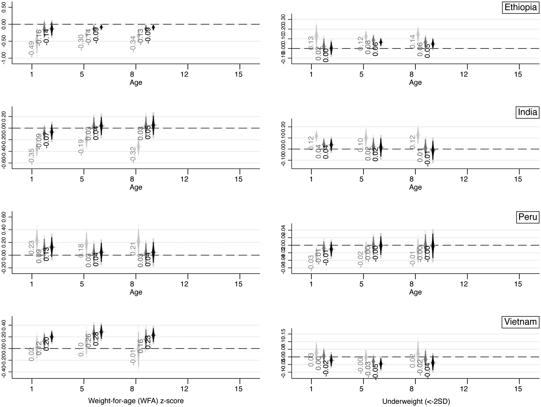
Association between parental educational similarity and children’s WFA z-scores (left) and prevalence of underweight (right) at different ages – coefficient on homogamy reported, without controls (NC, light grey), controlling for maternal and paternal education (EDU, dark grey), and with full set of controls (FULL, black).

Notes: For each age, three coefficients on parental educational homogamy are reported: one with no controls (light grey, left), one with mother and father’s education as controls (dark grey, middle), and one with the full set of controls (black, right). 90, 95, and 99 percent (longest bars) confidence intervals reported.

References

- Abufhele A, Castro AF, & Pesando LM (2020). Parental educational similarity and infant health in Chile: Evidence from administrative records: 1990–2015. Working Paper (manuscript currently revised and resubmitted).
- Aizer A, Stroud L, & Buka S (2016). Maternal stress and child outcomes: Evidence from siblings. Journal of Human Resources, 51(3), 523–555. [DOI] [PMC free article] [PubMed] [Google Scholar]
- Anand P, Behrman JR, Dang HAH, & Jones S (2018). Varied patterns of catch-up in child growth: Evidence from Young Lives. Social Science and Medicine, 214(July), 206–213. [DOI] [PubMed] [Google Scholar]
- Barnett I, Ariana P, Petrou S, Penny ME, Duc LT, Galab S, … Boyden J (2013). Cohort profile: The young lives study. International Journal of Epidemiology, 42(3), 701–708. [DOI] [PubMed] [Google Scholar]
- Beck A, & González-Sancho C (2009). Educational assortative mating and children’s school readiness. Center for Research on Child Wellbeing Working Paper. [Google Scholar]
- Becker GS (1981). A Treatise on the Family. Cambridge, MA: Harvard University Press. [Google Scholar]
- Behrman JA (2019). Mother’s relative educational status and early childhood height-for-age z acores: A decomposition of change over time. Population Research and Policy Review. [Google Scholar]
- Beijers R, Jansen J, Riksen-Walraven M, & De Weerth C (2010). Maternal prenatal anxiety and stress predict infant illnesses and health complaints. Pediatrics, 126(2). [DOI] [PubMed] [Google Scholar]
- Bratsberg B, Markussen S, Raaum O, Røed K, & Røgeberg O (2018). Trends in assortative mating and offspring outcomes. IZA Discussion Paper Series, (11753). [Google Scholar]
- Breen R, & Salazar L (2011). Educational assortative mating and earnings inequality in the United States. American Journal of Sociology, 117(3), 808–843. [Google Scholar]
- Briones K (2018). A guide to Young Lives rounds 1 to 5 constructed files. Young Lives Technical Note 48, 1–31. [Google Scholar]
- Cantarutti A, Franchi M, Monzio Compagnoni M, Merlino L, & Corrao G (2017). Mother’s education and the risk of several neonatal outcomes: An evidence from an Italian population-based study. BMC Pregnancy and Childbirth, 17(1), 1–10. [DOI] [PMC free article] [PubMed] [Google Scholar]
- Case A, & Paxson C (2002). Parental behavior and child health. Health Affairs, 21(2), 164–178. [DOI] [PubMed] [Google Scholar]
- Case A, & Paxson C (2010). Causes and consequences of early-life health. Demography, 47(Supplement), 65–85. [DOI] [PMC free article] [PubMed] [Google Scholar]
- Casterline JB, Williams L, & McDonald P (1986). The age difference between spouses: Variations among developing countries. Population Studies, 40(3), 353–374. [Google Scholar]
- Chen Y, & Li H (2009). Mother’s education and child health: Is there a nurturing effect? Journal of Health Economics, 28(2), 413–426. [DOI] [PubMed] [Google Scholar]
- Chevalier A (2004). Parental education and child’s education: A natural expriment. IZA Discussion Paper Series, (1153). [Google Scholar]
- Chevalier A, & O’Sullivan V (2007). Mother’s education and birth weight. IZA Discussion Paper Series, (2640). [Google Scholar]
- Chou SY, Liu JT, Grossman M, & Joyce T (2010). Parental education and child health: Evidence from a natural experiment in Taiwan. American Economic Journal: Applied Economics, 2(1), 33–61. [DOI] [PMC free article] [PubMed] [Google Scholar]
- Cochrane SH, Leslie J, & O’Hara DJ (1982). Parental education and child health: Intracountry evidence. Health Policy and Education, 2, 213–250. [DOI] [PubMed] [Google Scholar]
- Cole TJ, Flegal KM, Nicholls D, & Jackson AA (2007). Body mass index cut offs to define thinness in children and adolescents: International survey. British Medical Journal, 335(7612), 194–197. [DOI] [PMC free article] [PubMed] [Google Scholar]
- Cools S, & Kotsadam A (2017). Resources and intimate partner violence in sub-Saharan Africa. World Development, 95, 211–230. [Google Scholar]
- Corno L, Hildebrandt N, & Voena A (2020). Age of marriage, weather shocks, and the direction of marriage payments. Econometrica, 88(3), 879–915. [Google Scholar]
- Currie J, & Moretti E (2003). Mother’s education and the intergenerational transmission of human capital: Evidence from college openings. Quarterly Journal of Economics, 118(4), 1495–1532. [Google Scholar]
- Dancause KN, Laplante DP, Oremus C, Fraser S, Brunet A, & King S (2011). Disaster-related prenatal maternal stress influences birth outcomes: Project Ice Storm. Early Human Development, 87(12), 813–820. [DOI] [PubMed] [Google Scholar]
- De Hauw Y, Grow A, & Van Bavel J (2017). The reversed gender gap in education and assortative mating in Europe. European Journal of Population, 1–41. [DOI] [PMC free article] [PubMed] [Google Scholar]
- De Onis M, & Branca F (2016). Childhood stunting: A global perspective. Maternal and Child Nutrition, 12, 12–26. [DOI] [PMC free article] [PubMed] [Google Scholar]
- De Onis M, Onyango AW, Borghi E, Siyam A, Nishida C, & Siekmann J (2007). Development of a WHO growth reference for school-aged children and adolescents. Bulletin of the World Health Organization, 85(9), 660–667. [DOI] [PMC free article] [PubMed] [Google Scholar]
- Desai S, & Alva S (1998). Maternal education and child health: Is there a strong causal relationship? Demography, 35(1), 71–81. [PubMed] [Google Scholar]
- Eika L, Mogstad M, & Zafar B (2019). Educational assortative mating and household income inequality. Journal of Political Economy, 127(6), 000–000. [Google Scholar]
- Esteve A, Garcia J, & Permanyer I (2012). The reversal of the gender gap in education and its impact on union formation: the end of hypergamy. Population and Development Review, 38(3), 535–546. [Google Scholar]
- Furlong KR, Anderson LN, Kang H, Lebovic G, Parkin PC, Maguire JL, … Birken CS (2016). BMI-for-Age and weight-for-length in children 0 to 2 years. Pediatrics, 138(1). [DOI] [PubMed] [Google Scholar]
- Furstenberg FF (2005). Banking on families: How families generate and distribute social capital. Journal of Marriage and Family, 67, 809–821. [Google Scholar]
- Ganguli I, Hausmann R, & Viarengo M (2014). Closing the gender gap in education: What is the state of gaps in labour force participation for women, wives and mothers? International Labor Review, 153(2). [Google Scholar]
- Garfinkel I, Glei DA, & McLanahan S (2002). Assortative mating among unmarried parents. Journal of Population Economics, 15, 417–432. [Google Scholar]
- Georgiadis A, Benny L, Duc LT, Galab S, Reddy P, & Woldehanna T (2017). Growth recovery and faltering though early adolescence in low- and middle-income countries: Determinants and implications for cognitive development. Social Science and Medicine, 179, 81–90. [DOI] [PMC free article] [PubMed] [Google Scholar]
- Goldstein JR, & Harknett K (2006). Parenting across racial and class lines: Assortative mating patterns of new parents who are married, cohabiting, dating or no longer romantically involved. Social Forces, 85(1), 121–143. [Google Scholar]
- Gullickson A, & Torche F (2014). Patterns of racial and educational assortative mating in Brazil. Demography, 51(3), 835–856. [DOI] [PubMed] [Google Scholar]
- Güneş PM (2015). The role of maternal education in child health: Evidence from a compulsory schooling law. Economics of Education Review, 47, 1–16. [Google Scholar]
- Gutman LM, McLoyd VC, & Tokoyawa T (2005). Financial strain, neighborhood stress, parenting behaviors, and adolescent adjustment in urban African American families. Journal of Research on Adolescence, 15(4), 425–449. [Google Scholar]
- Haushofer J, & Fehr E (2014). On the psychology of poverty. Science, 344(6186), 862–867. [DOI] [PubMed] [Google Scholar]
- Headey D, Hoddinott J, Ali D, Tesfaye R, & Dereje M (2015). The other Asian enigma: Explaining the rapid reduction of undernutrition in Bangladesh. World Development, 66, 749–761. [Google Scholar]
- Kemptner D, & Marcus J (2013). Spillover effects of maternal education on child’s health and health behavior. Review of Economics of the Household, 11(1), 29–52. [Google Scholar]
- Kerr ME (2000). One’s Family Story: A Primer on Bowen Theory. Washington, DC: The Bowen Center for the Study of the Family. [Google Scholar]
- Kumar A, & Singh A (2013). Decomposing the gap in childhood undernutrition between poor and non-poor in urban India, 2005–06. PLoS ONE, 8(5). [DOI] [PMC free article] [PubMed] [Google Scholar]
- Lindeboom M, Llena-Nozal A, & van der Klaauw B (2009). Parental education and child health: Evidence from a schooling reform. Journal of Health Economics, 28(1), 109–131. [DOI] [PubMed] [Google Scholar]
- Mare RD (2016). Educational homogamy in two gilded ages: Evidence from inter-generational social mobility data. The ANNALS of the American Academy of Political and Social Science, 663(1), 117–139. [Google Scholar]
- Martin A, Ryan RM, & Brooks-Gunn J (2007). The joint influence of mother and father parenting on child cognitive outcomes at age 5. Early Childhood Research Quarterly, 22(4), 423–439. [Google Scholar]
- Minuchin P (1985). Families and individual development: Provocations from the field of family therapy. Child Development, 56(2Case_2010.pdf), 289–302. [PubMed] [Google Scholar]
- Nievar MA, & Luster T (2006). Developmental processes in African American families: An application of McLoyd’s theoretical model. Journal of Marriage and Family, 68(2), 320–331. [Google Scholar]
- Persson P, & Rossin-Slater M (2018). Family ruptures, stress, and the mental health of the next generation. American Economic Review, 108(4–5), 1214–11252. [PubMed] [Google Scholar]
- Pesando LM (2021). Educational assortative mating in sub-Saharan Africa: Compositional changes and implications for household wealth inequality. Demography (forthcoming). [DOI] [PMC free article] [PubMed] [Google Scholar]
- Pesando LM, & Abufhele A (2019). Household determinants of teen marriage: Sister effects across four low- and middle-income countries. Studies in Family Planning, 50(2), 113–136. [DOI] [PubMed] [Google Scholar]
- Petrou S, & Kupek E (2010). Poverty and childhood undernutrition in developing countries: A multi-national cohort study. Social Science and Medicine, 71(7), 1366–1373. [DOI] [PubMed] [Google Scholar]
- Rauscher E (2020). Why who marries whom matters: Effects of educational assortative mating on infant health in the United States 1969–1994. Social Forces, 98(3), 1143–1173. [DOI] [PMC free article] [PubMed] [Google Scholar]
- Reynolds SA, Andersen C, Behrman J, Singh A, Stein AD, Benny L, … Fernald LCH (2017). Disparities in children’s vocabulary and height in relation to household wealth and parental schooling: A longitudinal study in four low- and middle-income countries. SSM - Population Health, 3(February), 767–786. [DOI] [PMC free article] [PubMed] [Google Scholar]
- Rosenfeld MJ (2008). Racial, educational and religious endogamy in the United States: A comparative historical perspective. Social Forces, 87(1), 1–31. [Google Scholar]
- Ruiz M, Goldblatt P, Morrison J, Kukla L, Švancara J, Riitta-Järvelin M, … Pikhart H (2015).
- Ruiz M, Goldblatt P, Morrison J, Kukla L, Švancara J, Riitta-Järvelin M, … Pikhart H (2015). Mother’s education and the risk of preterm and small for gestational age birth: A DRIVERS meta-analysis of 12 European cohorts. Journal of Epidemiology and Community Health, 69(9), 826–833. [DOI] [PMC free article] [PubMed] [Google Scholar]
- Schott WB, Crookston BT, Lundeen EA, Stein AD, & Behrman JR (2013). Periods of child growth up to age 8 years in Ethiopia, India, Peru and Vietnam: Key distal household and community factors. Social Science and Medicine, 97, 278–287. [DOI] [PMC free article] [PubMed] [Google Scholar]
- Schwartz CR (2013). Trends and variation in assortative mating: Causes and consequences. Annual Review of Sociology, 39(1), 451–470. [Google Scholar]
- Schwartz CR, & Mare RD (2005). Trends in educational assortative marriage from 1940 to 2003. Demography, 42(4), 621–646. [DOI] [PubMed] [Google Scholar]
- Seckl JR (1998). Physiologic programming of the fetus. Clinics in Perinatology, 25(4), 939–964. [PubMed] [Google Scholar]
- Smits J, & Park H (2009). Five decades of educational assortative mating in 10 East Asian societies. Social Forces, 88(1), 227–255. [Google Scholar]
- Torche F (2010). Educational assortative mating and economic inequality: A comparative analysis of three latin American countries. Demography, 47(2), 481–502. [DOI] [PMC free article] [PubMed] [Google Scholar]
- Torche F (2011). The effect of maternal stress on birth outcomes: Exploiting a natural experiment. Demography, 48(4), 1473–1491. [DOI] [PubMed] [Google Scholar]
- Torche F, & Kleinhaus K (2012). Prenatal stress, gestational age and secondary sex ratio: The sex-specific effects of exposure to a natural disaster in early pregnancy. Human Reproduction, 27(2), 558–567. [DOI] [PMC free article] [PubMed] [Google Scholar]
- Wilson I, & Huttly S (2004). Young Lives: A case study of sample design for longitudinal research. Young Lives Working Paper N. 10, 1–16. [Google Scholar]
- World Health Organization. (2006). WHO child growth standards: Methods and development. EN Technical Report, 1–336. [Google Scholar]
- Young Lives. (2017). A Guide to Young Lives Research. (May), 1–46. Retrieved from www.younglives.org.uk [Google Scholar]
- Zhang H, Ho PSY, & Yip PSF (2012). Does similarity breed marital and sexual satisfaction? Journal of Sex Research, 49(6), 583–593. [DOI] [PubMed] [Google Scholar]