Abstract
Timely and accurate detection of an epidemic/pandemic is always desired to prevent its spread. For the detection of any disease, there can be more than one approach including deep learning models. However, transparency/interpretability of the reasoning process of a deep learning model related to health science is a necessity. Thus, we introduce an interpretable deep learning model: Gen-ProtoPNet. Gen-ProtoPNet is closely related to two interpretable deep learning models: ProtoPNet and NP-ProtoPNet The latter two models use prototypes of spacial dimension
 and the distance function
 . In our model, we use a generalized version of the distance function
 that enables us to use prototypes of any type of spacial dimensions, that is, square spacial dimensions and rectangular spacial dimensions to classify an input image. The accuracy and precision that our model receives is on par with the best performing non-interpretable deep learning models when we tested the models on the dataset of
 -ray images. Our model attains the highest accuracy of 87.27% on classification of three classes of images, that is close to the accuracy of 88.42% attained by a non-interpretable model on the classification of the given dataset.
Keywords: Covid-19, pneumonia, image recognition, X-ray, prototypical part, deep learning
I. Introduction
The world is still struggling with the pandemic of Covid-19 and its variants, such as: B.1.1.7, B.1.351 and P.1 [18]. Many facets efforts have been made to control and contain the disease. These efforts include detection of the virus. Many models have been proposed to detect Covid-19 from medical images, see [4], [12], [22], [23], [25], [36], [37], [40], [58]. These models lack the interpretability of their predictions, but the interpretability of the models related to public health is utmost important. The objective of this work is to find an interpretable method to do image classification so that we can tell why an image is classified in a certain way. In this work, we introduce an interpretable deep learning model: generalized prototypical part network (Gen-ProtoPNet), and experiment it over the dataset of three different classes of
 -rays, see Section V. Gen-ProtoPNet is a close variation of ProtoPNet [7] and NP-ProtoPNet [41]. To predict the class of a test image, ProtoPNet calculates the similarity scores between learned prototypical parts (with square spacial dimensions
 ) of images from each class and parts of the test image using
 distance function. These similarity scores are multiplied with a weight matrix to establish a positive connection between prototypes and logits of their correct classes, and a zero connection between prototypes and logits of incorrect classes. However, NP-ProtoPNet establishes a negative connection between prototypes and logits of incorrect classes instead of a zero connection between prototypes and logits of incorrect classes, unlike ProtoPnet. Both ProtoPNet and NP-ProtoPNet use the distance function
 to calculate similarity scores, and they use prototypes of square spacial dimensions
 . In this work, we use a generalized version of the distance function
 , see Section V-A. The generalized version of the distance function enables us to use prototypical parts of any type of spacial dimensions, that is, rectangular spacial dimensions as well as square spacial dimensions. In this work, a prototypical part or a prototype will represent a part, a patch or a section of an image. The similarity score between a learned prototypical part and an image is considered better if the sum of squares of the differences between the corresponding pixel values of the prototype and a patch of the image is lesser. We are motivated not to use
 spacial dimensions for prototypes due to following two reasons: (i) the model gives lesser accuracy; (ii) higher accuracy with the wrong reasoning process.
First, small spacial dimensions (
 ) can lead to lesser accuracy because images of objects from different classes can have small parts similar that can lead to good similarity score between patches of a test image and patches of images from wrong classes that gives rise to wrong classification. For example, most of the
 -ray images have some part black as a background, see Figure 2. Therefore, the use of prototypical parts of spacial dimensions
 can give good similarity scores between patches of an input image and patches of images from wrong classes, because all the images have some part black. Another example, images of birds from different sea bird species can share same background on most part of the images. So, the use of prototypes of spacial dimension
 can wrongly give high similarity score between patches of a test image and patches of images form wrong classes, because mostly such images have water as a background.
FIGURE 2.
Similarity between learned prototypical parts and an
 -ray image of a pneumonia patient.
Second, the images of objects from completely different classes do not have even small patches similar, and the classification of the images can be made just on the basis of the background in the images instead of identifying the objects themselves. For example, any patch of the images of birds of a sea specie is not similar to any patch of the images of birds of a jungle specie. Therefore, the use of the prototypical parts of the spacial dimensions
 can separate a sea bird image from an image of a jungle bird just on the basis of the background in the images instead of identifying the birds themselves.
On the other hand, using prototypical parts of spacial dimension of the biggest possible size can also reduce the accuracy because then the prototypical part will be an image itself instead of being a part of an image. Therefore, there can be only few images that are very similar to such a prototype whose size is equal to the size of an image, but a part of an image with smaller size can be similar to the parts of many other images. Since a prototype represents a part of an image, the optimum value for the spacial dimensions of a prototype lies between
 and the biggest possible dimension (in our case, the biggest possible spacial dimension of prototypes is
 ), that is, the spacial dimension of the output of the convolution layers of the baseline models, see Section V.
The use of prototypical parts of spacial dimension bigger than
 gives us better accuracy and precision as compared to prototypical parts of spacial dimensions
 that are used in ProtoPNet and NP-ProtoPNet, see Section VIII.
II. Literature Review
Some techniques have been developed to interpret the convolution neural networks, such as: posthoc interpretability analysis and attention-based interpretability. In posthoc analysis of a deep learning model, one interprets a trained convolution neural network after the predictions with the fitting explanations of the reasoning behind classifications made by the model. Posthoc analysis is made with various techniques, such as: activation maximization [10], [19], [27], [35], [43], [48], [57], deconvolution [59], and saliency visualization [39], [43], [45], [46]. However, these posthoc visualization methods fail to explain the actual reasoning process behind the classifications made by the models.
Many models have been developed that build attention-based interpretability, such as: class activation maps and part-based models. An attention-based interpretability model attempts to highlight the parts of an input image on which the network focuses [11], [15], [16], [21], [38], [42], [47], [56], [60]–[63]. Nevertheless, these models have serious drawback of not pointing out the prototypical parts that are similar to patches of the image on which the model focuses.
Li et al. [28], proposed a deep learning architecture that builds case-based reasoning into a neural network. Then Chen et al. [7] along with the authors of the above paper made a considerable improvement in their model ProtoPNet, whereby the network makes prediction by comparing image patches with the learned prototypes. The authors of this paper introduced a model NP-ProtoPNet [41] that is a close variation of ProtoPNet.
As mentioned in the introduction, many networks have been emerged to classify the
 -ray images of Covid-19 patients along with
 -ray images of normal people and pneumonia patients, see [4], [12], [22], [23], [25], [36], [37], [40], [41], [58]. A study summarizes some papers on Covid-19, and it points out some problems, such as: lack of reliable and adequate amount of data for deep learning algorithms [5]. Some studies related to Covid-19 and IoT are also worth mentioning [1]–[3], [6], [8], [26], [30]–[33], [49]. In this work, we also experimented our model over the same dataset that is used in some of the above Covid-19 related articles.
III. Data
We trained and evaluated our network on the dataset of frontal chest
 -ray images of Covid-19 patients [13], pneumonia patients and normal persons [24]. The dataset of chest
 -ray images from Kaggle database [24] has 3875 and 1341 training images of pneumonia patients and normal persons, respectively. Also, the dataset has 390 and 234 test images of pneumonia patients and normal persons, respectively. The other database [13] has 930 medical images of Covid-19 patients. These medical images include, frontal chest
 -ray images, CT-scan images, side
 -ray images and few obscure (completely black or white) images. Among the medical images of Covid-19 patients, we selected only 748 frontal chest
 -ray images. As compared to the number of chest
 -ray images of pneumonia patients and normal persons, the number of chest
 -ray images of Covid-19 patients was much lesser. Therefore, to balance the data, a copy of the chest
 -ray images of Covid-19 patients was included to form a dataset of 1496 images. The 1496 frontal chest
 -ray images of Covid-19 patients were divided into train and test sets of 1248 and 248 images, respectively. All these images form the three classes, labeled as: Covid, Normal and Pneumonia. We resized the images to dimension
 .
.
IV. Working Principle and Novelty of Gen-ProtoPNet
For
 -ray images given in figures 1 and 2, ProtoPNet is able to recognize many patches of the test image that looks like parts of images of some class. ProtoPNet decides the class of a test image on the basis of a weighted combination of the similarity scores [7]. Similarity scores between patches of a test image and prototypical parts (with square spacial dimensions
 ) are acquired with maximization of the inverted
 distances between them. The novelty of our model Gen-ProtoPNet is as follows.
-
1)
Our model uses a generalized version (see Section V-A) of the distance function
 .
. -
2)
It uses prototypes of both types of spacial dimensions, that is, it uses prototypes of square spacial dimensions as well as rectangular spacial dimensions.
-
3)
It uses prototypes with spacial dimensions bigger than the square spacial dimensions
 , that is, either height or width of prototypes is bigger than 1.
The use of generalized distance function and spacial dimensions bigger than
 helped our model to improve its performance.
FIGURE 1.
Similarity between learned prototypical parts and an
 -ray image of a Covid-19 patient.
V. Methodology
We construct our model over the following models: VGG-16, VGG-19 [44], ResNet-34, ResNet-152 [17], DenseNet-121, or DenseNet-161 [20] (initialized with filters pretrained on ImageNet [9]). We call these models baseline or base models. In the Figure 3, we see that the model comprises of the convolution layers of any of the above base model that are followed by an additional
 layer (we denote these convolution layers together by
 whose parameters are collectively denoted by
 ) and then these convolution layers are followed by a prototype layer
 and a fully connected layer
 with weight matrix
 and no bias. The prototype layer
 is a generalized convolution layer, [14], [34]. The activation function ReLU is used for all the convolution layers. Note that, Gen-ProtoPNet has only one additional
 convolution layer unlike ProtoPNet.
FIGURE 3.

Gen-ProtoPNet architecture.
Let
 be an input image and
 is the output of the convolutional layers
 . If
. If
 is the depth of the output
 then the shape of
 is
is
 . For example, when Gen-ProtoPNet is constructed over the convolution layers of VGG-16 then the depth of
 is 512. Although, there is one additional
 convolution layer, but it is not used to reduce the depth of
 . Therefore, the depth of each prototype is set equal to the depth of output of the regular convolution layers. We pick 10 prototypical parts for each class of images, and this number is randomly chosen. That is, Gen-ProtoPNet learns 30 prototypes. The set of prototypes is denoted by
 . These prototypical parts should catch enough relevant parts for recognizing a test image. The shape of each prototype is
 , where
 , that is, both
 and
and
 are not simultaneously equal to 1. The spacial dimensions of
 are
are
 , whereas the spacial dimensions of the prototypes are
 . Thus, every prototypical part
 will be used to represent some prototypical activation pattern in a patch of
 . Hence, every prototypical part
 can be considered as a representation of a patch of some image.
In Figure 3, the prototypical part
 is similar to a part of the
 -ray of a Covid-19 patient. The original/source image of the prototypical part
 is also given in the Figure 3. The patch
 is the part of the original image, that is enclosed in a rectangle with green boundaries. Similarly, the patches
 and
and
 are parts of the original images given in the same row in the Figure 3. For the output
 of a test image
 , the
, the
 -th prototypical unit
 in
in
 calculates (with the generalized version of
 ) distances between the prototypical part
 and each patch of
 . These distances are inverted into similarity scores which results in an activation map of similarity scores. More the activation value, stronger the presence of a prototype in the image
 . This activation map preserves the spatial relation of the convolutional output, and can be upsampled to the size of the input image to produce a heat map that identifies which part of the input image is most similar to the learned prototype [7]. These regions are enclosed in the green rectangles on the source images. The activation map is max-pooled to reduce to a single similarity score, that is, there is only one similarity score for each prototype. In the fully connected layer
 , the similarity scores produced with global max-pooling are multiplied with the matrix
 to get the logits, then these logits give prediction after normalization with softmax.
The
 -th entry
 of the weight matrix
 connects
 -th prototype and the logit of
 -th class. The similarity scores (after max-pooling) form a column matrix
 , see Section VI. The logits of Covid, Normal and Pneumoina classes are obtained from the multiplication of first, second and third rows of
 with the matrix
 . In Figure 3, the test image is an
 -ray image of a Covid-19 patient. The prototypes
 ,
,
 and
and
 are prototypes of images from Covid, Normal and Pneumonia classes, respectively. The similarity scores between patches of the input image and patches
 ,
,
 and
and
 are 0.042843, 0.000106 and 0.000082, respectively. The complete list of similarity scores is provided in the similarity score matrix
 , see Section VI. The logits for the classes Covid, Normal and Pneumonia are 0.751309, −0.624092 and −0.620997, respectively.
A. Mathematical Formulation and the Training of Gen-ProtoPNet
In this section, we describe the generalization of the distance function
 (Euclidean distance) using base model VGG-16. Also, we present the mathematical formulation and training steps of our algorithm with the generalized distance function. Gen-ProtoPNet is constructed over the regular convolution layers whose output channels have spacial dimension
 , see Section V. Let
 be an input image. Let
 (
(
 ) be of the shape (
 , 7, 7), where
 is the depth of
 . Consider a prototype
 of the shape (
 ,
,
 ,
,
 ). Let
 and
and
 be
be
 and
and
 pixels of
 th tensor of
 and
and
 , respectively. Let
 be obtained by convolving
 over
over
 with stride size equal to 1. Then
 is a tensor of the shape (
 ,
,
 ,
,
 ). Therefore, each feature map of
 has (
has (
 )(
)(
 ) pixels. For
 ,
,
 and
and
 ;
;
 pixel
pixel
 of the
 th feature map of
 is given by:
 |
Let
 be obtained from the Hadamard multiplication of feature maps of
 with themselves. Let
 be obtained from
 by convolving (over
 ) all 1’s filter of the shape of prototypes with stride size equal to 1. Note that,
 is the sum of the patches of
 of the shape
 over all feature maps. Therefore, the shape of
 is
is
 , and
, and
 pixel
pixel
 of
of
 is given by:
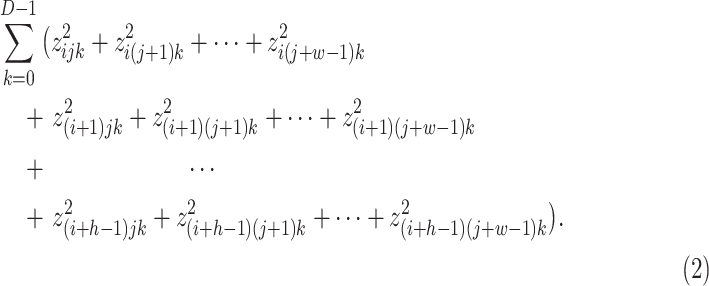 |
Note that,
 has
has
 patches of the spacial dimension
 . Hence, the distance
 between
 patch
patch
 (say) of
 and a prototype
 is given by:
 |
The equations 1 and 2 give the values of
 and
and
 . Thus,
 and
and
 . Therefore, by equation 3,
 |
If the spacial dimension of a prototype
 is
is
 then
then
 and
and
 , which is the square of
 distance between a patch of
 and the prototype
 , where
 . Therefore, if the spacial dimensions of
 are not equal to
 then
then
 is a generalization of the distance function
 . The distance function
 is used in both ProtoPNet and NP-ProtoPNet to find distances of prototypes (spacial dimension
 ) and the patches of images. The prototypical unit
 calculates:
 |
Alternatively,
 |
The equation 4 tells us that if
 is similar to
 then
then
 is smaller. The following three steps are performed to train our algorithm.
1). Stochastic Gradient Descent (SGD) of Every Layer Before Dense Layer
At this stage of learning, Gen-ProtoPNet aim to learns important features of the image while salient parts cluster near their respective classes. To attain this aim, Gen-ProtoPNet collectively optimize the parameters
 and
and
 in
in
 using SGD. Let
 be a set of image and
 is a set of corresponding labels, and
 . Our goal is to solve the following optimization problem:
 |
where ClstCt and SepCt are as follows:
 |
The decrease in cluster cost clusters prototypical parts around their correct class, see equation 6, whereas the decrease in separation cost attempts to separate prototypical parts from their incorrect class [7], see equation 7. The decrease in the cross entropy gives better classifications, see equation 5. The coefficients
 is set equal to 0.8 and the coefficient
 belongs to the interval (0.08, 0.8). Let
 be the set of prototypical parts of the images that belong to
 -th class. For a class
 , we put
 for all
 with
with
 and
and
 for all
 with
with
 . Since similarity scores are nonnegative, in this way Gen-ProtoPNet learns a meaningful latent space [7].
2). Push of Prototypical Parts
To see which part of the training images are used as prototypes, Gen-ProtoPNet projects every prototype
 onto the patch of the output
 that has smallest distance from
 , and
, and
 belong to class of
 [7]. That is, for every prototype
 of class
 , Gen-ProtoPNet perform the following update:
 |
3). Optimization of the Last Layer
To rely only on positive connections between prototypes and logits. We aim to make negative connection
 to 0 for all
 with
with
 . We perform this process after fixing all the parameters of convolution layers and prototype layer, and aim to optimize [7]:
 |
B. Selection of an Image Patch as a Prototype
Suppose
 is the source image of a prototype
 . The patch of
 that is most activated by the prototype
 is used for the visualization of
 . Its activation value must be at least 92nd percentile of all the activation values (before max-pooling) of
 [7].
[7].
VI. Explanation of the Reasoning Process of Gen-ProtoPNet With an Example
We constructed our model over six baseline models. We trained and tested our model for 500 epochs. The model VGG-16 is used as a baseline model to run the experiments explained in this example. However, the measures of the performance of the model with the other baseline model are given in the Table 1.
TABLE 1. Comparison of the Performances of Gen-ProtoPNet and the Other Models.
| Base (B) | Dimension/Metrics | Gen-ProtoPNet+B | NP-ProtoPNet[27] + B | ProtoPNet[2] + B | B only |
|---|---|---|---|---|---|
| VGG-16 |
 |
||||
| accuracy | 85.89 | 84.63 | 79.73 | 82.45 | |
| precision | 0.99 | 0.97 | 0.87 | 0.97 | |
| recall | 0.98 | 0.99 | 0.92 | 0.98 | |
| Fl-score | 0.98 | 0.97 | 0.89 | 0.97 | |
| VGG-19 |
 |
||||
| accuracy | 84.40 | 88.99 | 81.78 | 82.68 | |
| precision | 0.99 | 0.91 | 0.84 | 0.96 | |
| recall | 0.98 | 0.96 | 0.95 | 0.98 | |
| Fl-score | 0.98 | 0.93 | 0.89 | 0.97 | |
| ResNet-34 |
 |
||||
| accuracy | 85.20 ± 0.23 | 84.29 ± 0.10 | 82.90 ± 0.21 | 84.89 ± 0.12 | |
| precision | 0.99 | 0.99 | 0.98 | 0.99 | |
| recall | 0.98 | 0.99 | 0.99 | 0.99 | |
| Fl-score | 0.98 | 0.99 | 0.98 | 0.99 | |
| ResNet-152 |
 |
||||
| accuracy | 86.70 ± 0.18 | 86.40 ± 0.12 | 83.60 ± 0.34 | 88.03 ± 0.24 | |
| precision | 0.98 | 0.99 | 0.87 | 0.98 | |
| recall | 0.99 | 0.99 | 0.89 | 0.99 | |
| Fl-score | 0.98 | 0.99 | 0.88 | 0.98 | |
| DenseNet-121 |
 |
||||
| accuracy | 87.04 ± 0.13 | 86.47 ± 0.11 | 85.90 ± 0.36 | 88.41 ± 0.12 | |
| precision | 0.98 | 0.99 | 0.98 | 0.99 | |
| recall | 0.99 | 0.98 | 0.98 | 0.99 | |
| Fl-score | 0.98 | 0.98 | 0.98 | 0.99 | |
| DenseNet-161 |
 |
||||
| accuracy | 87.27 ± 0.23 | 87.04 ± 0.21 | 86.58 ± 0.32 | 88.42 ± 0.23 | |
| precision | 0.97 | 0.97 | 0.95 | 0.99 | |
| recall | 0.99 | 0.99 | 0.96 | 0.99 | |
| Fl-score | 0.97 | 0.97 | 0.96 | 0.99 |
In the Figure 4, the test image in the first column is a member of the Covid class. In next column, each image is the test image with a rectangle (at a certain place) on it. The rectangles have green boundaries. The pixels enclosed by such a rectangle on an image in the second column correspond to the pixels on the original image in the fourth column and same row. In fact the patch enclosed by a rectangle on an image in the fourth column is the patch from where a prototype (third column and same row) is projected. The fifth column consists of similarity scores that are explained in Section V. The similarity scores of a prototype
 is the
 -th entry of the similarity score matrix
 (say). The sixth column consists of weights of Covid class. Since Covid is a first class these weight are entries of first row of
 . The multiplication of the first row of the weight matrix
 with
with
 gives logit for the Covid class. Similarly, logit for Normal and Pneumonia classes can be obtained by multiplying second and third row of the weight matrix
 with the matrix
 , respectively. Hence, the logits for the first, second and third classes are 0.752591, −0.627040 and −0.623544, respectively. The matrix
 and transpose of
 that we obtain from our experiments are:
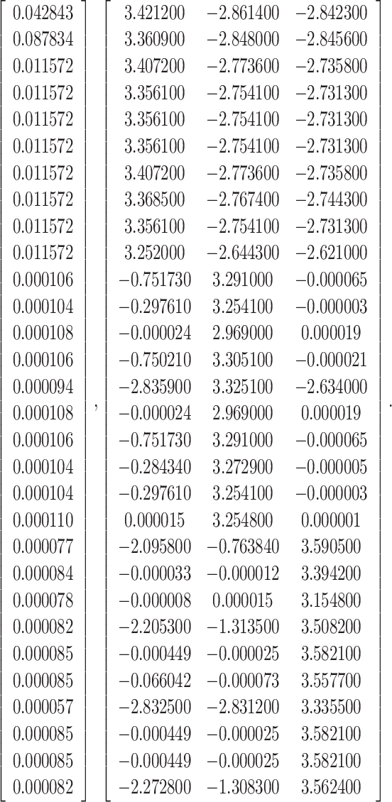 |
FIGURE 4.
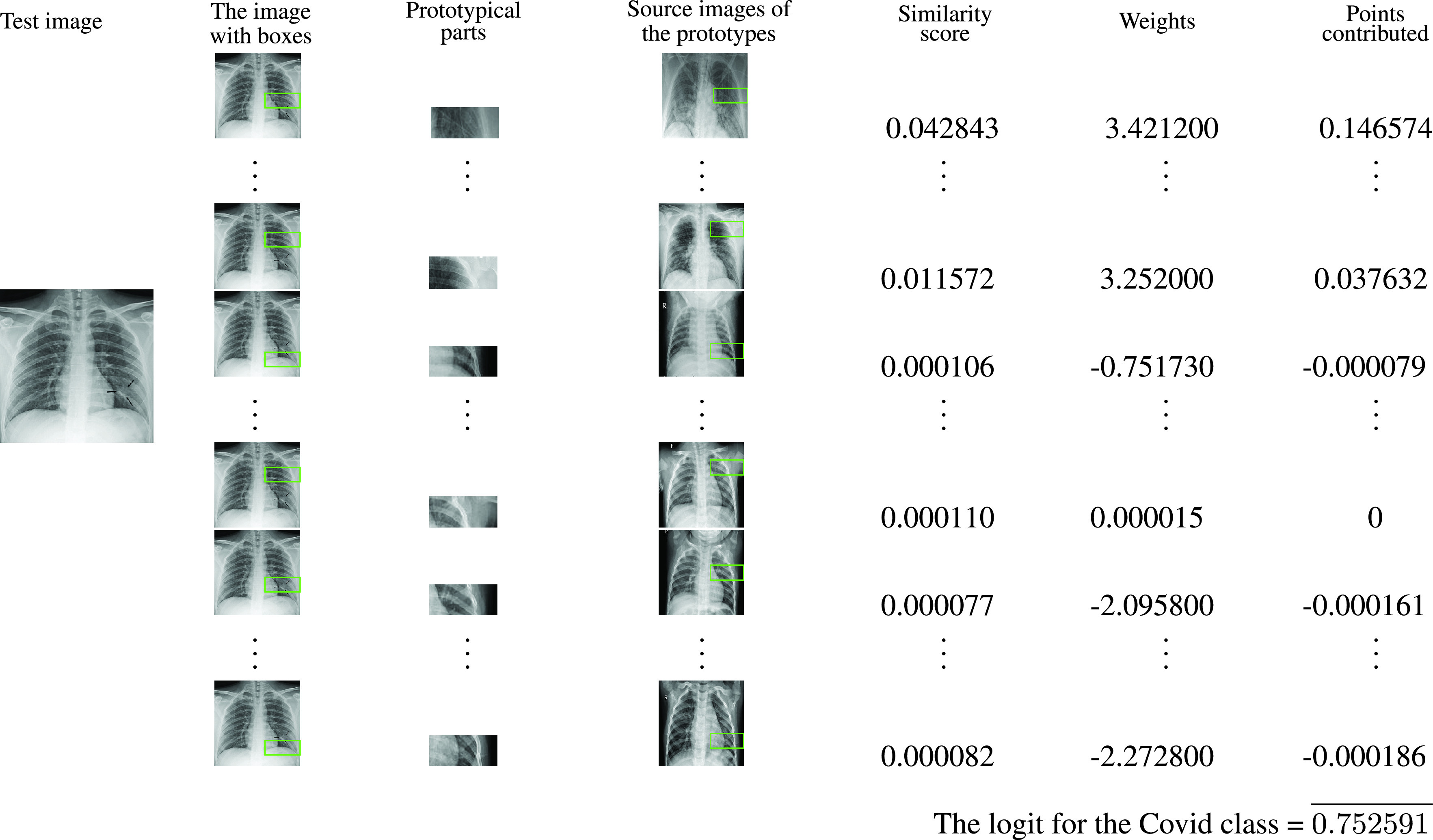
The explanation of the reasoning process of our network with an
 -ray image of a Covid-19 patient.
VII. The Performance Description With Confusion Matrices
The comparison of the performance of Gen-ProtoPNet with NP-ProtoPNet, ProtoPNet and the base models is made with some metrics, such as: accuracy, precision, recall and F1-score. The confusion matrices are also used to outline the performance of Gen-ProtoPNet. A confusion matrix is an array that is used to describe the performance of a classification model on a set of test data for which the true values are known [54].
True positive (TP) is the number of items correctly labeled as belonging to the positive class, that is, the items are predicted to belong to a class when they actually belong to that class. True negative (
 ) is the number of items for which the model correctly predict the negative classes, that is, the items are predicted to not belonging to a class when they actually belong to other classes, see [55]. Note that, in non-binary classifications,
 and
and
 are the diagonal entries of the confusion matrix. False positive (
 ) is the number of items incorrectly predicted as belonging to the positive class. False negative (
 ) is the number of items incorrectly predicted as not belonging to the positive class, see [52]. The metrics accuracy, precision and recall in terms of the above positives and negatives are:
 |
F1-score is the harmonic mean of precision and recall, that is,
 , see [53].
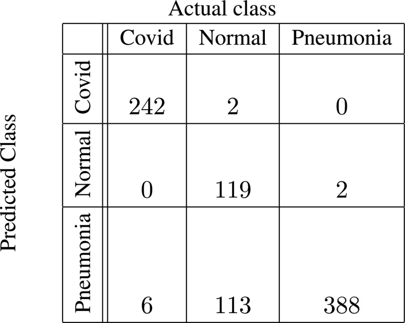
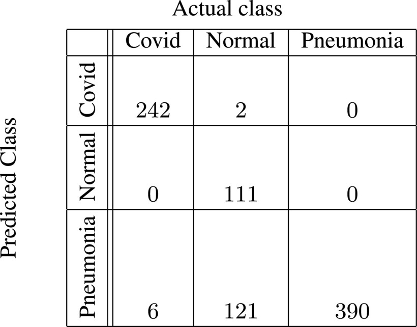
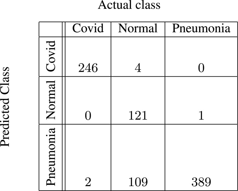
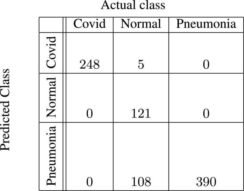
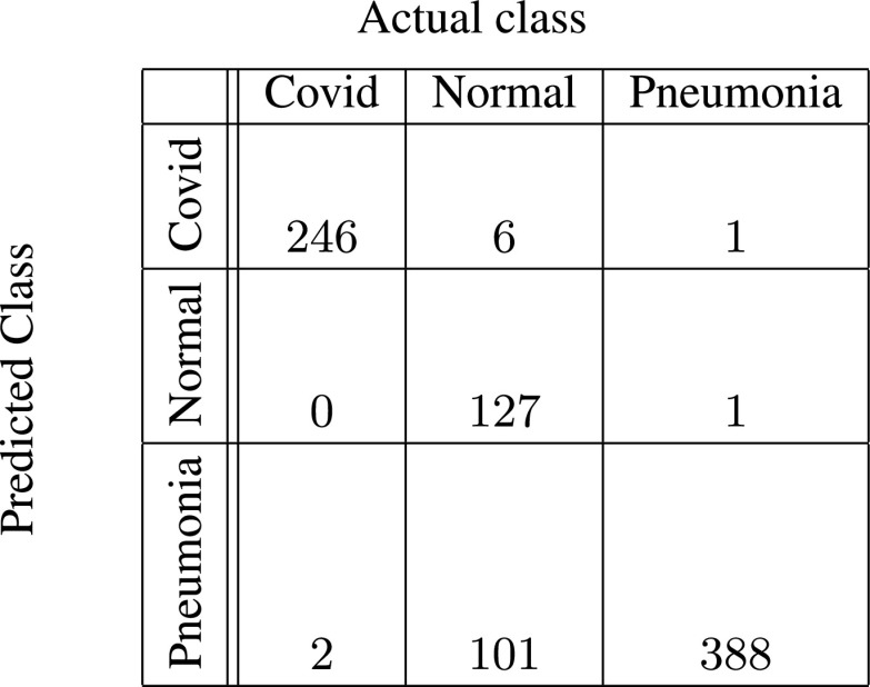
In figures 5–10, the confusion matrices give visualization of the performance of Gen-ProtoPNet with the six baselines. Let
 be any of the following six confusion matrices. Suppose
 entry of the confusion matrix
 is given by
 . Therefore,
 for the first class (Covid) are
 , and
, and
 are
are
 . In addition,
 and
and
 for the first class are
 and
and
 respectively. Next, we describe the confusion matrix (given in Figure 5) for Gen-ProtoPNet when constructed over baseline VGG-16. Total correct predictions made by Gen-ProtoPNet with baseline VGG-16 are 749 (=242 + 119 + 388), see Figure 5. Total number of test images are 872, see Section V. Thus, the accuracy is 85.89%. The above definitions and Figure 5 give us the precision, recall and F1-score equal to 0.99, 0.98 and 0.98, respectively. Similarly, the metrics for Gen-ProtoPNet with the other baselines can be determined from Figures 6–10.
FIGURE 5.
Gen-ProtoPNet with base VGG-16.
FIGURE 6.
Gen-ProtoPNet with base VGG-19.
FIGURE 7.
Gen-ProtoPNet with ResNet-34.
FIGURE 8.
Gen-ProtoPNet with ResNet-152.
FIGURE 9.
Gen-ProtoPNet with DenseNet-121.
FIGURE 10.
Gen-ProtoPNet with DenseNet-161.
VIII. Comparison of the Performance of Gen-ProtoPNet With the Performance of NP-ProtoPNet, ProtoPNet and the Baselines
The convolution layers of several neural networks can be used to build the models Gen-ProtoPNet, NP-ProtoPNet and ProtoPNet. As stated in Section V, we trained and tested Gen-ProtoPNet with the baseline models over the datesets of the
 -rays [13], [24]. Also, NP-ProtoPNet and ProtoPNet were examined over the same datasets and with the same base models. We trained and tested all models that are compared in Table 1 for 500 epochs.
The measures of the performances of the models (Gen-ProtoPNet, NP-ProtoPNet and ProtoPNet with the six base models) in the metrics can be found in Table 1. Also, the measures of the performance the base models themselves are given in Table 1. We explain the Table 1 with an account of the performance of each of these models with base model VGG-16. However, the measures of the performance of these models with the other five base models are also given in Table 1.
In the second column of the Table 1, the spacial dimensions of prototypes corresponding to each base model are given. For example, when Gen-ProtoPNet is constructed over the base model VGG-16, and prototypes have spacial dimension
 then the accuracy, precision, recall and F1-score of Gen-ProtoPNet are 85.89, 0.99, 0.98 and 0.98, respectively. Similarly, the measures of the performances of the models NP-ProtoPNet and ProtoPNet with baseline model VGG-16 in the metrics accuracy, precision, recall and F1-score are 84.63, 0.97, 0.99, 0.97, and 79.93, 0.87, 0.92, 0.89, respectively. Also, the measures of the performances of VGG-16 itself (Base only) in the metrics accuracy, precision, recall and F1-score are 82.45, 0.97, 0.98 and 0.97, respectively.
The performance of Gen-ProtoPNet is improved over ProtoPNet with all the base models. Also, the performance of Gen-ProtoPNet is better than the performance of NP-ProtoPNet with some baseline models, and in two cases its performance is better than the performance of the baseline models themselves.
IX. Graphical Comparison of the Accuracies of the Models
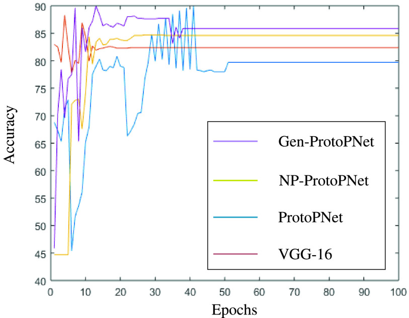
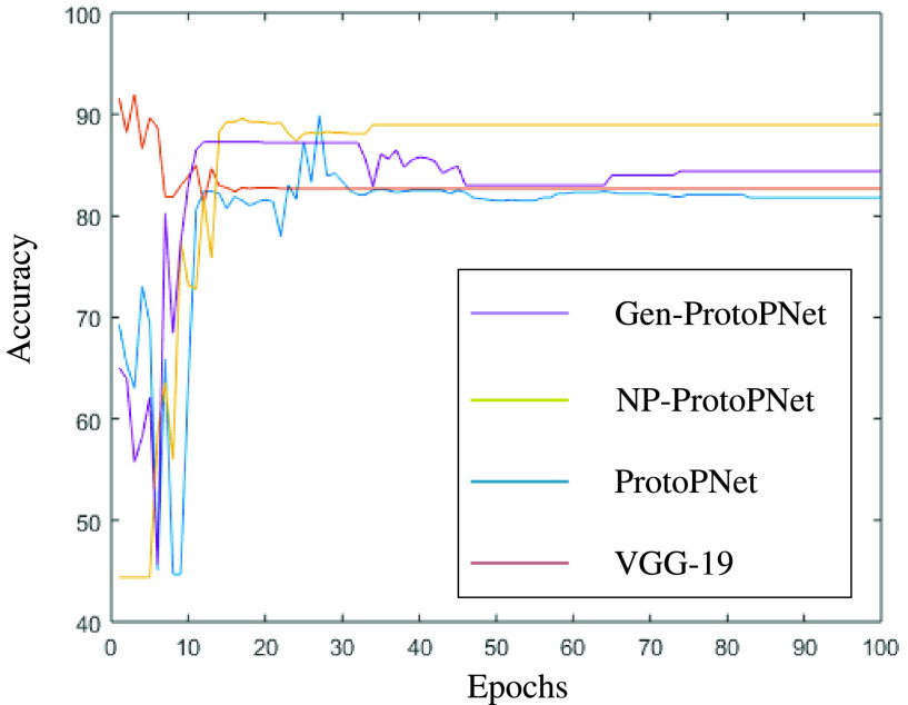
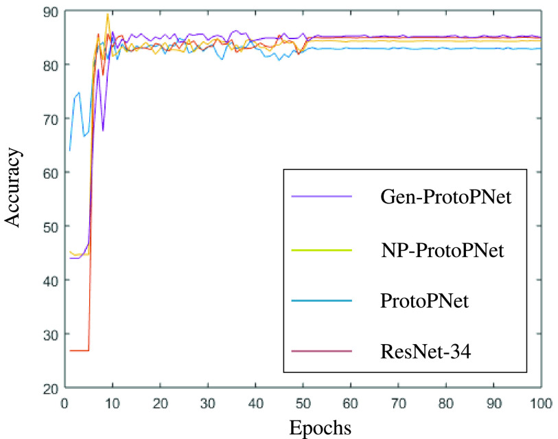
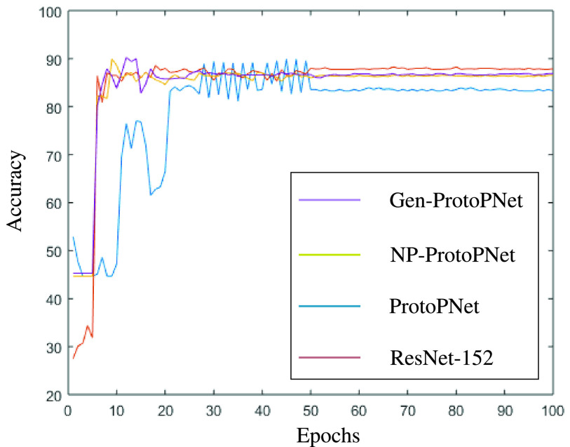
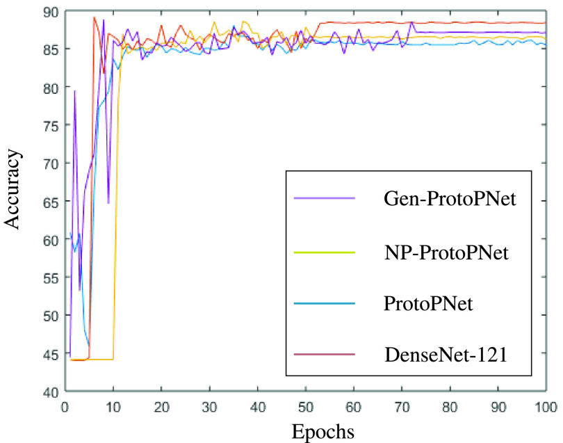
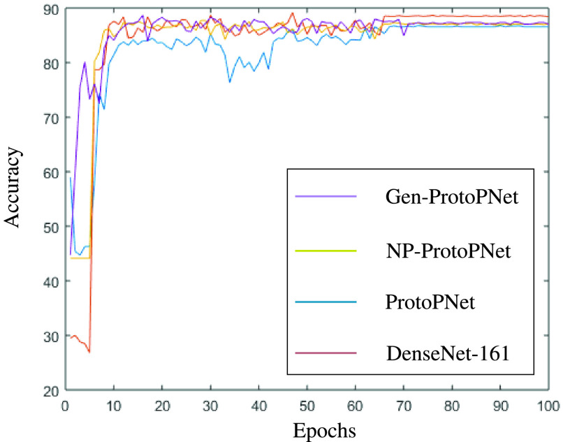
In this section, a graphical comparison of the accuracies of Gen-ProtoPNet with the other models is provided over 100 epochs. In the figures 11–16, the curves of colors purple, yellow, blue and brown sketch the accuracies of Gen-ProtoPNet, NP-ProtoPNet, ProtoPNet and the baselines. For example, in Figure 11, the accuracies of Gen-ProtoPNet, NP-ProtoPNet and ProtoPNet with the base model VGG-16, and the base model VGG-16 itself are depicted.
FIGURE 11.
Accuracy comparison with baseline VGG-16.
FIGURE 12.
Accuracy comparison with baseline VGG-19.
FIGURE 13.
Accuracy comparison with baseline ResNet-34.
FIGURE 14.
Accuracy comparison with baseline ResNet-152.
FIGURE 15.
Accuracy comparison with baseline DenseNet-121.
FIGURE 16.
Accuracy comparison with baseline DenseNet-161.
The performance in accuracy of Gen-ProtoPNet is the highest with the baseline model VGG-16 and second highest for the remaining base models except VGG-19. Therefore, the curve depicting the accuracy for Gen-PrortoPNet is the highest for base model VGG-16 and second highest for the other base models.
The accuracies given by these models become stable before 100 epochs. Although, we experimented these models for 500 epochs, but the comparison of the accuracies of these models is outlined in the figures 11–16 only for first 100 epochs to make the shape of the curves more clearer in the beginning as accuracy of each of these models stabilizes before 100 epochs.
X. Limitations
The convex optimization of the last layer of our model takes considerable time during the training of our model. Our experiments show that zero connection between similarity scores and incorrect classes is hard to achieve during the training process. However, this technique of convex optimization of the last layer is adopted from ProtoPNet model that has already been published in one of the top conferences [7].
XI. Conclusion
Gen-ProtoPNet is closely related to two interpretable deep learning models ProtoPNet and NP-ProtoPNet that calculate the similarity scores between prototypes of spacial dimension
 and patches of an input image by finding the
 distance between the prototypes and the patches. In our model, we use a generalized version of the distance function
 that enables us to use prototypes of any type of spacial dimensions, that is, square spacial dimensions and rectangular spacial dimensions. The use of rectangular spacial dimensions of prototypes enabled our model to improve its performance over ProtoPNet model.
Biographies

Gurmail Singh received the M.Sc. degree in mathematics from Panjab University, Chandigarh, India, in 2003, the M.Phil. degree in mathematics from Madurai Kamaraj University, India, in 2007, and the Ph.D. degree in algebra from the University of Regina, Canada, in 2015.
From 2007 to 2009, he was a Lecturer with the B. L. M. Girls College, Nawanshahr, India. After qualifying UGC-Net, in 2009, he served as an Assistant Professor for a period of two years with the Khalsa College, Garhshankar, India. Since 2015, he has been working as a Research Associate with the Department of Computer Science, and the Department of Mathematics and Statistics. He is currently working as a Postdoctoral researcher with the Kin-Choong Yow’s laboratory of Artificial Intelligence Research, Faculty of Engineering and Applied Science.

Kin-Choong Yow (Senior Member, IEEE) received the B.Eng. (Elect.) degree (Hons.) from the National University of Singapore, in 1993, and the Ph.D. degree from the University of Cambridge, U.K., in 1998.
From 1999 to 2005, he served as the Sub-Dean for computer engineering with Nanyang Technological University (NTU), Singapore, and the Associate Dean for admissions with NTU, from 2006 to 2008. In September 2018, he joined the University of Regina, where he is currently an Associate Professor with the Faculty of Engineering and Applied Science. Prior to joining the University of Regina, he was an Associate Professor with the Gwangju Institute of Science and Technology (GIST), Republic of Korea, from 2013 to 2018; a Professor with the Shenzhen Institutes of Advanced Technology (SIAT), China, from 2012 to 2013; and an Associate Professor with NTU, from 1998 to 2013. He has published over 90 top quality international journal articles and conference papers. His research interests include artificial general intelligence and smart environments. He is a member of APEGS and ACM. He has served as a Reviewer for a number of premier journals and conferences, including the IEEE Wireless Communications and the IEEE Transactions on Education. He has been invited to give presentations at various scientific meetings and workshops, such as ACIRS, from 2018 to 2019; ICSPIC, in 2018; and ICATME, in 2021. He is the Editor-in-Chief of the Journal of Advances in Information Technology (JAIT).
Funding Statement
We acknowledge the support of the Natural Sciences and Engineering Research Council of Canada (NSERC), funding reference number DDG-2020-00034. Cette recherche a été financée par le Conseil de recherches en sciences naturelles et en génie du Canada (CRSNG), numéro de référence DDG-2020-00034.
References
- [1].Abdulkareem K. H., Mohammed M. A., Salim A., Arif M., Geman O., Gupta D., and Khanna A., “Realizing an effective COVID-19 diagnosis system based on machine learning and IOT in smart hospital environment,” IEEE Internet Things J., early access, Jan. 11, 2021, doi: 10.1109/JIOT.2021.3050775. [DOI] [PMC free article] [PubMed]
- [2].Al-Waisy A. S., Mohammed M. A., Al-Fahdawi S., Maashi M. S., Garcia-Zapirain B., Abdulkareem K. H., Mostafa S. A., Kumar N. M., and Le D.-N., “COVID-DeepNet: Hybrid multimodal deep learning system for improving COVID-19 pneumonia detection in chest X-ray images,” Comput., Mater. Continua, vol. 67, no. 2, pp. 2409–2429, 2021, doi: 10.32604/cmc.2021.012955. [DOI] [Google Scholar]
- [3].Al-Waisy A. S., Al-Fahdawi S., Mohammed M. A., Abdulkareem K. H., Mostafa S. A., Maashi M. S., Arif M., and Garcia-Zapirain B., “COVID-CheXNet: Hybrid deep learning framework for identifying COVID-19 virus in chest X-rays images,” Soft Comput., pp. 1–16, Nov. 2020, doi: 10.1007/s00500-020-05424-3. [DOI] [PMC free article] [PubMed]
- [4].Azemin M. Z. C., Hassan R., Tamrin M. I. M., and Ali M. A. M., “COVID-19 deep learning prediction model using publicly available radiologist-adjudicated chest X-ray images as training data: Preliminary findings,” Int. J. Biomed. Imag., vol. 2020, pp. 1–7, Aug. 2020, doi: 10.1155/2020/8828855. [DOI] [PMC free article] [PubMed] [Google Scholar]
- [5].Bhattacharya S., Maddikunta P. K. R., Pham Q.-V., Gadekallu T. R., Krishnan S. R. S., Chowdhary C. L., Alazab M., and Piran M. J., “Deep learning and medical image processing for coronavirus (COVID-19) pandemic: A survey,” Sustain. Cities Soc., vol. 65, Feb. 2021, Art. no. 102589. [DOI] [PMC free article] [PubMed] [Google Scholar]
- [6].Chaudhary Y., Mehta M., Sharma R., Gupta D., Khanna A., and Rodrigues J. J. P. C., “Efficient-CovidNet: Deep learning based COVID-19 detection from chest X-ray images,” in Proc. IEEE Int. Conf. E-Health Netw., Appl. Services (HEALTHCOM), Mar. 2021, pp. 1–6, doi: 10.1109/HEALTHCOM49281.2021.9398980. [DOI] [Google Scholar]
- [7].Chen C., Li O., Tao C., Barnett A. J., Su J., and Rudin C., “This looks like that: Deep learning for interpretable image recognition,” in Proc. 33rd Conf. Neural Inf. Process. Syst. (NIPS), 2019, pp. 1–12. [Google Scholar]
- [8].Dansana D., Kumar R., Bhattacharjee A., Hemanth D. J., Gupta D., Khanna A., and Castillo O., “Early diagnosis of COVID-19-affected patients based on X-ray and computed tomography images using deep learning algorithm,” Soft Comput., Aug. 2020, doi: 10.1007/s00500-020-05275-y. [DOI] [PMC free article] [PubMed]
- [9].Deng J., Dong W., Socher R., Li L.-J., Li K., and Fei-Fei L., “ImageNet: A large-scale hierarchical image database,” in Proc. IEEE Conf. Comput. Vis. Pattern Recognit. (CVPR), Jun. 2009, pp. 248–255. [Google Scholar]
- [10].Erhan D., Bengio Y., Courville A., and Vincent P., “Visualizing higher-layer features of a deep network,” presented at the Workshop Learn. Feature Hierarchies 26th Int. Conf. Mach. Learn. (ICML), Montreal, QC, Canada, Jun. 2009. [Google Scholar]
- [11].Fu J., Zheng H., and Mei T., “Look closer to see better: Recurrent attention convolutional neural network for fine-grained image recognition,” in Proc. IEEE Conf. Comput. Vis. Pattern Recognit. (CVPR), Jul. 2017, pp. 4438–4446. [Google Scholar]
- [12].Cohen J. P., Dao L., Roth K., Morrison P., Bengio Y., Abbasi A. F., Shen B., Mahsa H. K., Ghassemi M., Li H., and Duong T., “Predicting COVID-19 pneumonia severity on chest X-ray with deep learning,” Cureus, vol. 12, no. 7, p. e9448, Jul. 2020, doi: 10.7759/cureus.9448. [DOI] [PMC free article] [PubMed] [Google Scholar]
- [13].Cohen J. P., Morrison P., and Dao L.. (Aug. 24, 2020). COVID-19 Image Data Collection. [Online]. Available: https://github.com/ieee8023/covid-chestxray-dataset [Google Scholar]
- [14].Ghiasi-Shirazi K., “Generalizing the convolution operator in convolutional neural networks,” Neural Process. Lett., vol. 50, no. 3, pp. 2627–2646, Dec. 2019. [Google Scholar]
- [15].Girshick R., “Fast R-CNN,” in Proc. IEEE Int. Conf. Comput. Vis. (ICCV), Dec. 2015, pp. 1440–1448. [Google Scholar]
- [16].Girshick R., Donahue J., Darrell T., and Malik J., “Rich feature hierarchies for accurate object detection and semantic segmentation,” in Proc. IEEE Conf. Comput. Vis. Pattern Recognit. (CVPR), Jun. 2014, pp. 580–587. [Google Scholar]
- [17].He K., Zhang X., Ren S., and Sun J., “Deep residual learning for image recognition,” in Proc. IEEE Conf. Comput. Vis. Pattern Recognit. (CVPR), Jun. 2016, pp. 770–778. [Google Scholar]
- [18].Health. (Apr. 2, 2021). How Many New Coronavirus Variants are There? [Online]. Available: https://www.healthline.com/health/how-many-strains-of-covid-are-there
- [19].Hinton G. E., “A practical guide to training restricted Boltzmann machines,” in Neural Networks: Tricks of the Trade. Berlin, Germany: Springer, 2012, pp. 599–619. [Google Scholar]
- [20].Huang G., Liu Z., Van Der Maaten L., and Weinberger K. Q., “Densely connected convolutional networks,” in Proc. IEEE Conf. Comput. Vis. Pattern Recognit. (CVPR), Jul. 2017, pp. 4700–4708. [Google Scholar]
- [21].Huang S., Xu Z., Tao D., and Zhang Y., “Part-stacked CNN for fine-grained visual categorization,” in Proc. IEEE Conf. Comput. Vis. Pattern Recognit. (CVPR), Jun. 2016, pp. 1173–1182. [Google Scholar]
- [22].Jain G., Mittal D., Thakur D., and Mittal M. K., “A deep learning approach to detect COVID-19 coronavirus with X-ray images,” Biocybern. Biomed. Eng., vol. 40, no. 4, pp. 1391–1405, Oct. 2020. [DOI] [PMC free article] [PubMed] [Google Scholar]
- [23].Jain R., Gupta M., Taneja S., and Hemanth D. J., “Deep learning based detection and analysis of COVID-19 on chest X-ray images,” Appl. Intell., vol. 51, no. 3, pp. 1690–1700, Mar. 2021, doi: 10.1007/s10489-020-01902-1. [DOI] [PMC free article] [PubMed] [Google Scholar]
- [24].Kaggle. (Aug. 24, 2020). Chest X-Ray (Pneumoina). [Online]. Available: https://www.kaggle.com/allen-institute-for-ai/CORD-19-research-challenge
- [25].Kumar R., Arora R., Bansal V., Sahayasheela V., Buckchash H., Imran J., Narayanan N., Pandian G. N., and Raman B., “Accurate prediction of COVID-19 using chest X-ray images through deep feature learning model with SMOTE and machine learning classifiers,” medRxiv, pp. 1–10, Apr. 2020, doi: 10.1101/2020.04.13.20063461. [DOI]
- [26].Le D.-N., Parvathy V. S., Gupta D., Khanna A., Rodrigues J. J. P. C., and Shankar K., “IoT enabled depthwise separable convolution neural network with deep support vector machine for COVID-19 diagnosis and classification,” Int. J. Mach. Learn. Cybern., Jan. 2021, doi: 10.1007/s13042-020-01248-7. [DOI] [PMC free article] [PubMed]
- [27].Lee H., Grosse R., Ranganath R., and Ng A. Y., “Convolutional deep belief networks for scalable unsupervised learning of hierarchical representations,” in Proc. 26th Annu. Int. Conf. Mach. Learn. (ICML), 2009, pp. 609–616. [Google Scholar]
- [28].Li O., Liu H., Chen C., and Rudin C., “Deep learning for case-based reasoning through prototypes: A neural network that explains its predictions,” in Proc. 32nd AAAI Conf. Artif. Intell. (AAAI), 2018, pp. 1–8. [Google Scholar]
- [29].Liu X., Xia T., Wang J., Yang Y., Zhou F., and Lin Y., “Fully convolutional attention networks for fine-grained recognition,” 2016, arXiv:1603.06765. [Online]. Available: http://arxiv.org/abs/1603.06765
- [30].Mahanty C., Kumar R., Mishra B. K., Hemanth D. J., Gupta D., and Khanna A., “Prediction of COVID-19 active cases using exponential and non-linear growth models,” Expert Syst., vol. 66, no. 3, pp. 3289–3310, 2021, doi: 10.1111/exsy.12648. [DOI] [Google Scholar]
- [31].Mohammed M. A., Abdulkareem K. H., Garcia-Zapirain B., Mostafa S. A., Maashi M. S., Al-Waisy A. S., Subhi M. A., Mutlag A. A., and Le D.-N., “A comprehensive investigation of machine learning feature extraction and classification methods for automated diagnosis of COVID-19 based on X-ray images,” Comput., Mater. Continua, vol. 66, no. 3, pp. 3289–3310, 2021, doi: 10.32604/cmc.2021.012874. [DOI] [Google Scholar]
- [32].Mohammed M. A., Abdulkareem K. H., Al-Waisy A. S., Mostafa S. A., Al-Fahdawi S., Dinar A. M., Alhakami W., Baz A., Al-Mhiqani M. N., Alhakami H., Arbaiy N., Maashi M. S., Mutlag A. A., Garcia-Zapirain B., and De La Torre Diez I., “Benchmarking methodology for selection of optimal COVID-19 diagnostic model based on entropy and TOPSIS methods,” IEEE Access, vol. 8, pp. 99115–99131, 2020, doi: 10.1109/ACCESS.2020.2995597. [DOI] [Google Scholar]
- [33].Mukherjee R., Kundu A., Mukherjee I., Gupta D., Tiwari P., Khanna A., and Shorfuzzaman M., “IoT-cloud based healthcare model for COVID-19 detection: An enhanced k-nearest neighbour classifier based approach,” Computing, Apr. 2021, doi: 10.1007/s00607-021-00951-9. [DOI]
- [34].Nalaie K., Ghiasi-Shirazi K., and Akbarzadeh-T M.-R., “Efficient implementation of a generalized convolutional neural networks based on weighted Euclidean distance,” in Proc. 7th Int. Conf. Comput. Knowl. Eng. (ICCKE), Oct. 2017, pp. 211–216. [Google Scholar]
- [35].Nguyen A., Dosovitskiy A., Yosinski J., Brox T., and Clune J., “Synthesizing the preferred inputs for neurons in neural networks via deep generator networks,” in Proc. Adv. Neural Inf. Process. Syst. (NIPS), 2016, pp. 3387–3395. [Google Scholar]
- [36].Ozturk T., Talo M., Yildirim E. A., Baloglu U. B., Yildirim O., and Acharya U. R., “Automated detection of COVID-19 cases using deep neural networks with X-ray images,” Comput. Biol. Med., vol. 121, Jun. 2020, Art. no. 103792. [DOI] [PMC free article] [PubMed] [Google Scholar]
- [37].Reddy G. T., Bhattacharya S., Ramakrishnan S. S., Chowdhary C. L., Hakak S., Kaluri R., and Reddy M. P. K., “An ensemble based machine learning model for diabetic retinopathy classification,” in Proc. Int. Conf. Emerg. Trends Inf. Technol. Eng. (ic-ETITE), Feb. 2020, pp. 1–6. [Google Scholar]
- [38].Ren S., He K., Girshick R., and Sun J., “Faster R-CNN: Towards real-time object detection with region proposal networks,” in Proc. Adv. Neural Inf. Process. Syst. (NIPS), 2015, pp. 91–99. [DOI] [PubMed] [Google Scholar]
- [39].Selvaraju R. R., Cogswell M., Das A., Vedantam R., Parikh D., and Batra D., “Grad-CAM: Visual explanations from deep networks via gradient-based localization,” in Proc. IEEE Int. Conf. Comput. Vis. (ICCV), Oct. 2017, pp. 618–626. [Google Scholar]
- [40].Sharma A., Rani S., and Gupta D., “Artificial intelligence-based classification of chest X-ray images into COVID-19 and other infectious diseases,” Int. J. Biomed. Imag., vol. 2020, Oct. 2020, Art. no.8889023, doi: 10.1155/2020/8889023. [DOI] [PMC free article] [PubMed] [Google Scholar]
- [41].Singh G. and Yow K.-C., “These do not look like those: An interpretable deep learning model for image recognition,” IEEE Access, vol. 9, pp. 41482–41493, 2021, doi: 10.1109/ACCESS.2021.3064838. [DOI] [PMC free article] [PubMed] [Google Scholar]
- [42].Simon M. and Rodner E., “Neural activation constellations: Unsupervised part model discovery with convolutional networks,” in Proc. IEEE Int. Conf. Comput. Vis. (ICCV), Dec. 2015, pp. 1143–1151. [Google Scholar]
- [43].Simonyan K., Vedaldi A., and Zisserman A., “Deep inside convolutional networks: Visualising image classification models and saliency maps,” in Proc. 2nd Int. Conf. Learn. Represent. Workshop (ICLR Workshop), 2014, pp. 1–8. [Google Scholar]
- [44].Simonyan K. and Zisserman A., “Very deep convolutional networks for large-scale image recognition,” in Proc. 3rd Int. Conf. Learn. Represent. (ICLR), 2015, pp. 1–14. [Google Scholar]
- [45].Smilkov D., Thorat N., Kim B., Viégas F., and Wattenberg M., “SmoothGrad: Removing noise by adding noise,” 2017, arXiv:1706.03825. [Online]. Available: http://arxiv.org/abs/1706.03825
- [46].Sundararajan M., Taly A., and Yan Q., “Axiomatic attribution for deep networks,” in Proc. 34th Int. Conf. Mach. Learn., vol. 70, 2017, pp. 3319–3328. [Google Scholar]
- [47].Uijlings J. R. R., van de Sande K. E. A., Gevers T., and Smeulders A. W. M., “Selective search for object recognition,” Int. J. Comput. Vis., vol. 104, no. 2, pp. 154–171, Sep. 2013. [Google Scholar]
- [48].van den Oord A., Kalchbrenner N., and Kavukcuoglu K., “Pixel recurrent neural networks,” in Proc. 33rd Int. Conf. Mach. Learn. (ICML), 2016, pp. 1747–1756. [Google Scholar]
- [49].Waheed A., Goyal M., Gupta D., Khanna A., Al-Turjman F., and Pinheiro P. R., “CovidGAN: Data augmentation using auxiliary classifier GAN for improved COVID-19 detection,” IEEE Access, vol. 8, pp. 91916–91923, 2020, doi: 10.1109/ACCESS.2020.2994762. [DOI] [PMC free article] [PubMed] [Google Scholar]
- [50].Wexler R., “When a computer program keeps you in jail: How computers are harming criminal justice,” New York Times, Jun. 13, 2017, p. 27. [Google Scholar]
- [51].Wikipedia. (Apr. 2, 2021). Accuracy and Precision. [Online]. Available: https://en.wikipedia.org/wiki/Accuracy_and_precision
- [52].Wikipedia. (Apr. 2, 2021). Precision and Reacall. [Online]. Available: https://en.wikipedia.org/wiki/Precision_and_recall
- [53].Wikipedia. (Apr. 2, 2021). F-Score. [Online]. Available: https://en.wikipedia.org/wiki/F-score
- [54].Wikipedia. (Apr. 2, 2021). Confusion Matrix. [Online]. Available: https://wikipedia.org/wiki/Confusion_matrix
- [55].Wikipedia. (Apr. 2, 2021). Sensitivity and Specificity. [Online]. Available: https://en.wikipedia.org/wiki/Sensitivity_and_specificity
- [56].Xiao T., Xu Y., Yang K., Zhang J., Peng Y., and Zhang Z., “The application of two-level attention models in deep convolutional neural network for fine-grained image classification,” in Proc. IEEE Conf. Comput. Vis. Pattern Recognit. (CVPR), Jun. 2015, pp. 842–850. [Google Scholar]
- [57].Yosinski J., Clune J., Fuchs T., and Lipson H., “Understanding neural networks through deep visualization,” in Proc. Deep Learn. Workshop 32nd Int. Conf. Mach. Learn. (ICML), 2015, pp. 1–12. [Google Scholar]
- [58].Zebin T. and Rezvy S., “COVID-19 detection and disease progression visualization: Deep learning on chest X-rays for classification and coarse localization,” Int. J. Speech Technol., vol. 51, no. 2, pp. 1010–1021, Feb. 2021, doi: 10.1007/s10489-020-01867-1. [DOI] [PMC free article] [PubMed] [Google Scholar]
- [59].Zeiler M. D. and Fergus R., “Visualizing and understanding convolutional networks,” in Proc. Eur. Conf. Comput. Vis. (ECCV), 2014, pp. 818–833. [Google Scholar]
- [60].Zhang N., Donahue J., Girshick R., and Darrell T., “Part-based R-CNNs for fine-grained category detection,” in Proc. Eur. Conf. Comput. Vis. (ECCV). Cham, Switzerland: Springer, 2014, pp. 834–849. [Google Scholar]
- [61].Zheng H., Fu J., Mei T., and Luo J., “Learning multi-attention convolutional neural network for fine-grained image recognition,” in Proc. IEEE Int. Conf. Comput. Vis. (ICCV), Oct. 2017, pp. 5209–5217. [Google Scholar]
- [62].Zhou B., Khosla A., Lapedriza A., Oliva A., and Torralba A., “Learning deep features for discriminative localization,” in Proc. IEEE Conf. Comput. Vis. Pattern Recognit. (CVPR), Jun. 2016, pp. 2921–2929. [Google Scholar]
- [63].Zhou B., Sun Y., Bau D., and Torralba A., “Interpretable basis decomposition for visual explanation,” in Proc. Eur. Conf. Comput. Vis. (ECCV), 2018, pp. 119–134. [Google Scholar]


