δ¹⁵N of Chironomidae: An index of nitrogen sources and processing within watersheds for national aquatic monitoring programs

Abstract

Nitrogen (N) removal along flowpaths to aquatic ecosystems is an important regulating ecosystem service that can help reduce N pollution in the nation’s waterways, but can be challenging to measure at large spatial scales. Measurements that integrate N processing within watersheds would be particularly useful for assessing the magnitude of this vital service. Because most N removal processes cause isotopic fractionation, δ¹⁵N from basal food-chain organisms in aquatic ecosystems can provide information on both N sources and the degree of watershed N processing. As part of EPA’s National Aquatic Resource Surveys (NARS), we measured δ¹⁵N of Chironomidae collected from over 2000 lakes, rivers and streams across the continental USA. Using information on N inputs to watersheds and summer total N concentrations ([TN]) in the water column, we assessed where elevated chironomid δ¹⁵N would indicate N removal rather than possible enriched sources of N. Chironomid δ¹⁵N values ranged from −4 to +20 ‰, and were higher in rivers and streams than in lakes, indicating that N in rivers and streams underwent more processing and cycling that preferentially removes ¹⁴N than N in lakes. Chironomid δ¹⁵N increased with watershed size, N inputs, and water chemical components, and decreased as precipitation increased. In rivers and streams with high watershed N inputs, we found lower [TN] in streams with higher chironomid δ¹⁵N values, suggesting high rates of gaseous N loss such as denitrification. At low watershed N inputs, the pattern reversed; streams with elevated chironomid δ¹⁵N had higher [TN] than streams with lower chironomid δ¹⁵N, possibly indicating unknown sources elevated in δ¹⁵N such as legacy N, or waste from animals or humans. Chironomid δ¹⁵N values can be a valuable tool to assess integrated watershed-level N sources, input rates, and processing for water quality monitoring and assessment at large scales.

Graphical Abstract

1. INTRODUCTION

Nitrogen (N) pollution represents a major threat to aquatic ecosystems globally (Baron et al., 2011; Camargo and Alonso, 2006; Carpenter et al., 1998). In the USA, total nitrogen concentration ([TN]) in aquatic ecosystems is one of the main stressors associated with poor water quality in many of the nation’s lakes, rivers, and streams. The Environmental Protection Agency (EPA) National Rivers and Streams Assessment (NRSA), part of the National Aquatic Resource Surveys (NARS), reports on the condition of the nation’s rivers and streams, and using relative-risk analysis (Herlihy et al., 2019), the assessment estimated that the biological condition of 26% of total river and stream length across the USA could be improved by lowering [TN] in streams in 2008–2009, and 23% in 2013–2014 (U. S. Environmental Protection Agency, 2016b; U. S. Environmental Protection Agency, 2020). For lakes, the EPA’s National Lake Assessments (NLA) reported the biological condition of an estimated 22% and 16% of the nation’s lakes could be improved from lowering lake N concentrations in 2007 and 2012, respectively (U.S. Environmental Protection Agency, 2009; U.S. Environmental Protection Agency, 2016). Given the impact of N on aquatic ecosystems, we need a deeper understanding of the many pathways and cycles of N at broad spatial scales to address this consistent and continued N pollution problem.

Nitrogen concentrations and loads in aquatic ecosystems strongly reflect N inputs to the watershed (Bellmore et al., 2018; Boyer et al., 2002; Lin et al., 2021; Swaney et al., 2012; Van Breemen et al., 2002). These N inputs are dominated by agricultural inputs and the rate of inputs in the contiguous US (CONUS) has not significantly changed from 2002–2012 despite efforts to reduce N inputs to terrestrial systems (Sabo et al., 2019). Nitrogen releases beyond the intended uses are costly to society, with a large portion of that cost associated with N releases to aquatic ecosystems (Dodds et al., 2009; Sobota et al., 2015; Van Grinsven et al., 2013). Nitrogen inputs to watersheds account for roughly half of the variation in stream [TN] (Bellmore et al., 2018; Lin et al., 2021). However, given the biological demand for N, and its highly reactive and dynamic nature (Galloway et al., 2003), aquatic ecosystems can vary substantially in [TN], even when N inputs into watersheds are similar (Bellmore et al., 2018; Lin et al., 2021). Nitrogen processing and cycling along the flowpath between the point of application to the aquatic measurement point can result in very different amounts of N being transmitted to aquatic ecosystems (Boyer et al., 2002; Seitzinger et al., 2006). Landscape features such as wetlands and riparian areas are significant hotspots for processing N (Jordan et al., 2011; Mayer et al., 2007). Processes such as plant uptake, soil sequestration, ammonia volatilization and denitrification are all important process that can reduce N transport to aquatic ecosystems; however, determining which processes are important at broad spatial scales is difficult. This is particularly true of broad-scale water quality surveys such as EPA’s NARS, which include NRSA and NLA, and where sites across CONUS are selected using a probabilistic design and assessed once during a survey period. Additional measures that might help indicate N sources and extent of N processing would be useful to help identify watersheds that are either particularly efficient at retaining or removing N, and those where N is transported rapidly to water ways.

The stable isotope ratio of nitrogen (δ¹⁵N) has been used as an indicator of N processes that result in gaseous loss of N such as ammonia volatilization and denitrification (Bai et al., 2012; Houlton and Bai, 2009; Kendall et al., 2007; Yu et al., 2020). As a result of the large fractionation effects associated with gaseous loss of N (Denk et al., 2017), δ¹⁵N of the remaining N increases with increasing N cycling, and these effects accumulate in ecosystems overtime making δ¹⁵N values a good indicator of the intensity of N cycling over long temporal scales (Amundson et al., 2003; Bai et al., 2012; Robinson, 2001). A common application of δ¹⁵N is to identify different sources of N into aquatic systems (Kendall et al., 2007). Nitrogen that is newly fixed from the atmosphere by bacterial N fixation or chemical fertilizers has a low isotopic ratio, similar to that of atmospheric N₂ (0 ‰). Reactive N deposited from the atmosphere also have similarly low isotopic ratios (Holtgrieve et al., 2011). Other common sources of N represent pools that have been highly cycled or processed such as manure or sewage and have correspondingly higher isotopic ratios. This δ¹⁵N difference in sources makes it possible to attribute nitrogen to possible sources if processing of N remains minimal. However, given the highly reactive and cyclic nature of nitrogen in natural environments, minimal processing is rarely the case. Thus, any use of δ¹⁵N in broad scale surveys will have to contend with the fact that both sources and processing of N will cause the variation in δ¹⁵N. Nevertheless, Diebel and Vander Zanden (2009) used the δ¹⁵N of aquatic invertebrates in a broadscale survey of streams in Wisconsin, USA and found that most δ¹⁵N variation in invertebrates was related to gaseous N loss of inorganic fertilizer and not from sources of N elevated in ¹⁵N such as manure. On the other hand, Atkinson et al. (2014) found that the δ¹⁵N value of freshwater mussels were highly positively correlated with the net anthropogenic N inputs to the watershed. In association with landscape data on N inputs (Sabo et al., 2019), δ¹⁵N values of aquatic organisms can assist in understanding more about the source and/or processing of N found in aquatic ecosystems.

Here, we present the first national level δ¹⁵N dataset of invertebrates collected as part of the EPA NARS program. We limited our analysis to members of the family Chironomidae to minimize trophic influences on δ¹⁵N and because Chironomidae are ubiquitous within lakes, rivers and streams in across CONUS. Our goal was to understand how and when chironomid δ¹⁵N values indicate N pollution sources and/or N losses in the NARS program. Specifically, we explored the following three objectives:

1. Describe the magnitude of chironomid δ¹⁵N variation across CONUS to determine if it could be useful tool in understanding N pollution

2. Determine which factors drive chironomid δ¹⁵N variation: Landscape, waterbody attributes and/or foodweb attributes

3. Determine how chironomid δ¹⁵N can aid in explaining the variation in total N concentrations of lakes, rivers, and streams across the country.

2. MATERIALS AND METHODS

2.1. National Aquatic Resource Surveys

Chironomidae samples were obtained from across the contiguous United States using the benthic macroinvertebrate samples collected from EPA’s National Aquatic Resource Surveys of lakes, rivers, and streams in the summers (May-Oct) of 2007, 2008, and 2009 (U.S. Environmental Protection Agency, 2009). NLA lakes, and NRSA rivers and streams were distributed across CONUS and represent the national population of lakes, rivers, and streams (Figure 1). Each water body was selected using a probability-based survey design that ensures the sites represent the target population of these water bodies so that EPA can statistically assess the condition of the nation’s waters (Peck et al., 2013). We obtained enough (> 1 mg) chironomids for isotopic analysis from 1103 of the 2123 sites sampled in the 2008–2009 National Rivers and Streams Assessment (NRSA), and 943 of the 1157 sites sampled in the 2007 National Lakes Assessment (NLA) (Figure 1). Chironomid samples were not obtained from the remaining sites either because the processing labs did not retain and preserve the counted individuals, or chironomid numbers were not sufficient for isotopic analysis. Of those sites with chironomid samples, 86 NRSA sites and 67 NLA sites were revisited for assessment and had sufficient chironomids for site comparisons within a season.

Figure 1:

Map of NARS sample locations with sufficient chironomids in the benthic macroinvertebrate sample for isotopic analysis. NLA 2007 samples are indicated in red triangles while NRSA 2008–2009 samples are in black diamonds. Map colors represent nine aggregated ecoregions used by NARS.

2.1.1. Benthic Macroinvertebrate Sampling

For NLA lakes sampled in 2007, benthic macroinvertebrate samples were collected using a semi-quantitative sampling of the littoral zone of lakes using a 500 μm mesh D-frame dip net. The net was swept through 1 linear meter of the dominant habitat type (rocky/cobble/large woody debris, macrophyte beds, fine sediments, or leaf pack) at each of 10 equally spaced littoral sampling sites around the lake perimeter and composited into a single sample (U.S. Environmental Protection Agency, 2007b). For NRSA river and streams sampled in 2008 and 2009, boatable rivers were sampled in the same manner as lakes (1 m sweep of dominant habitat type) from the near shore areas of 11 equally spaced transects along the river sample reach. For wadeable streams, a 0.09 m² area kick sample was collected using a 500 μm mesh D-frame net at each of 11 transects equally distributed along the sample reach. As with lakes, samples from the multiple collection locations within a site were composited into a single sample for each stream or river (U.S. Environmental Protection Agency, 2007a). All samples were field processed to remove large detritus (rinsed and inspected for organisms) and preserved in 95% ethanol which has been shown to have minimal effects on isotopic values in macroinvertebrates (Syvaranta et al., 2008). Preserved composite samples were shipped to the taxonomic identification laboratories where samples were sorted, enumerated, and invertebrates identified to the lowest practical taxonomic level (typically genus) on a fixed count of 500 individuals. One laboratory (EcoAnalysts, Inc. https://www.ecoanalysts.com/) separated invertebrates into a glass vial and stored in 95% ethanol, whereas other taxonomic laboratories only retained a few mounted individual which could not be used for isotopic analysis. EcoAnalysts, Inc. conducted the majority of taxonomic analysis (Figure 1) and shipped chironomids to the Integrated Stable Isotope Research Facility (ISIRF) at EPA’s Pacific Ecological Systems Division in Corvallis, Oregon, for δ¹⁵N analysis (See section 2.2).

2.1.2. NARS data

For each NARS site where chironomids were obtained, we obtained NARS data (https://www.epa.gov/national-aquatic-resource-surveys/data-national-aquatic-resource-surveys). To address objective 2, understanding the drivers of chironomid δ¹⁵N variance, we categorized the data into three sets of drivers: landscape, water body and biological (i.e., food webs) (Table 1). For landscape, we used the NARS delineated watershed for each site and obtained watershed information such as watershed size, land-use, climate, and hydrologic data (i.e., baseflow index), many of which came from the StreamCat and LakeCat datasets (Hill et al., 2018; Hill et al., 2016). For the water body (lake or river/stream reach), we obtained water chemistry, water body morphology, and physical and nearshore habitat data from NARS databases (see U.S. Environmental Protection Agency, 2007a; U.S. Environmental Protection Agency, 2007b for field methods). We also utilized d-excess values (NRSA) and E:I (evaporation:inflow) values (NLA) calculated from δ¹⁸O and δ²H of water samples used for water chemistry as described in Brooks et al. (2014). These values were used to assess the influence of evaporative enrichment. For biological drivers, we focused on NARS data related to possible foodweb dynamics: chironomid δ¹³C, % chironomid individuals in various feeding guilds (i.e. scrapers, burrowers, predators), and NARS biological condition indices which are multi-metric indexes based on biological integrity (Stoddard et al., 2008).

Table 1.

Variables considered as possible drivers of Chironomid δ¹⁵N variation.

Landscape Variables	Units	Description
Basin Area	km2	Land area within the drainage basin to the lake, river or stream.
Wetland Area	%	Percent wetland area within the watershed (Combined herbaceous-NLCD95* + woody-NLCD90).
Forest Area	%	Percent forested area within the watershed (Combined Deciduous-NLCD41 + Evergreen-NLCD42 + Mixed-NLCD43).
Ag & Urban Area	%	Percent Agricultural (NLCD81+NLCD82) and Developed (NLCD21 + NLCD22 + NLCD23 + NLCD24) area within the watershed.
N Sources N with high δ15N	kg N/ha	Combined livestock and human waste N input rate‡.
N Sources with low δ15N	kg N/ha	Combined Farm and Urban fertilizer, Crop N fixation, and atmospheric deposition‡.
Precipitation	mm	PRISM† mean annual precipitation.
RH	%	PRISM mean annual relative humidity.
Temperature	°C	PRISM mean annual temperature.
Baseflow Index	%	The component of streamflow that can be attributed to groundwater discharge into lakes or streams. The Baseflow Index (BFI) is the ratio of baseflow to total flow, expressed as % within watershed.
Lake or Reach Variables
Total Phosphorus	μg/L	Total phosphorus concentration as measured by NARS⸙.
Total Nitrogen	μg/L	Total nitrogen concentration as measured by NARS.
Conductivity	μS/cm	Conductivity as measured by NARS.
Disolved Organic Carbon	mg/L	Disolved organic carbon as measured by NARS.
Lake Area	km2	Lake polygon area from USGS National Hydrography Dataset (NHD).
Depth	m	NLA: Lake depth as measured in the at the Index point (deepest location). NRSA: Mean thalweg depth of the sampled reach.
Water Residence Time	yrs	Lake water residence time determined from water isotopes⁑.
Evaporation Index	‰	NLA: Evaporation to inflow ratio (E:I)⁑. NRSA: d-excess⁑.
Riparian Condition		NRSA Riparian cover condition index☼.
Riparian-Littoral cover		NLA Riparian littoral condition index☼.
In-stream cover		NRSA instream cover index☼.
Riparian Disturbance		NARS Riparian disturbance index☼.
Biological Variables
Chironomid δ13C	‰	Carbon isotopic values of chironomidae
Taxa # found		Total number of distinct taxa found in the macroinvertebrate sample
Macroinvertebrate Condition Index		Multi-metric index indicating macroinvertebrate biological condition (Stoddard et al., 2008)
Lake Diatom Condition		NLA diatom condition index☼.
Chironomid Individuals		Number of Chironomid individuals found in macroinvertebrate sample
% Guilds	%	Percent of Chironomids belonging to 7 different functional feeding groups: climbers, sprawlers, predators, burrowers, collectors, filterers, and shredders

^*NLCD – National Land Cover Database (2006)

^‡Nitrogen inventory data from Sabo et al. (2019)

^†PRISM derived from 29 years of record (1971–2000)

^⸙NARS data and methods are available at https://www.epa.gov/national-aquatic-resource-surveys

^⁑Water isotope variables described in Brooks et al. (2014)

^☼NARS method details for these indices are available in the technical manuals (U. S. Environmental Protection Agency, 2016a; U.S. Environmental Protection Agency, 2010)

2.2. Isotopic Analysis

For stable isotopic analysis, ethanol was decanted, and chironomid samples were dried overnight in a 50°C drying oven. Samples were ground to a fine powder and isotopic analysis was conducted on 1 – 2 mg subsamples that were combusted in an elemental analyser (ECS 4010, Costech, Valencia, CA) and the resulting gases were analysed on an isotope ratio mass spectrometer (IRMS; Thermo Finnigan DELTAplus XP, Thermo Fisher Scientific) for δ¹⁵N and δ¹³C. All δ¹⁵N values are expressed relative to the standard AIR-N₂ and δ¹³C relative to Vienna Pee Dee Belemnite (VPDB):

$${\delta }^{15}\text{N}\mathit{\text{ or }}{\delta }^{13}\text{C }=\frac{{\text{R}}_{\text{sample}}}{{\text{R}}_{\text{standard}}}-1$$

where R is the ratio of ¹⁵N to ¹⁴N, or ¹³C to ¹²C atoms of the sample and the standard. Values are multiplied by 1000 to express in ‰. Three calibrated in-house laboratory standards ranging from 0.3 to 8.0 ‰ for δ¹⁵N and from −33.2 to −13.5 ‰ for δ¹³C were used to normalize samples to the international standard scale for each isotope. An independent in-house laboratory QC standard was used to assess accuracy in each sample set, and the exact QC standards varied over the 71 sample sets, but span the calibration range. Across all sample sets, accuracy averaged 0.08 ± 0.24 (sd) ‰ for δ¹⁵N and 0.11 ± 0.16 (sd) ‰ as determined from 71 QC standards. Precision (one standard deviation) of 82 sample duplicates was 0.3 and 0.6 ‰ for δ¹⁵N and δ¹³C, respectively. To assess variability of chironomids within a composite sample, 5–15 individual chironomids (i.e. not homogenized samples, numbers varied to reach the target weight of 1.2 mg) were weighed in duplicate on 62 samples. Precision on these samples were 0.6 and 0.9 ‰ for δ¹⁵N and δ¹³C, respectively. In addition, 153 sites were revisited on separate days during the assessment period and had sufficient chironomid samples to assess variation over the assessment period (86 for NRSA, and 67 for NLA). The standard deviations between these revisits were 1.3 and 1.7 ‰ for δ¹⁵N and δ¹³C, respectively.

2.3. Nitrogen Input Data

Total nitrogen inputs into NARS watersheds were calculated using the National Nutrient Inventory (NNI) for the year 2007 from Sabo et al. (2019). For the major nitrogen sources within the watersheds, we included agricultural and residential fertilizer, crop biological N fixation, land-applied manure, human waste, and atmospheric deposition. Input NNI rasters (30m resolution) were averaged across each NARS watershed and inputs for each source were given in average kg N ha⁻¹yr⁻¹ for the watershed. Total N inputs were calculated by summing all the sources, and we noted which source was the dominant for each watershed. We also separately summed sources likely to have higher δ¹⁵N values (land-applied manure and human waste) and sources likely to have lower δ¹⁵N values (agricultural and residential fertilizer, crop biological N fixation and atmospheric deposition).

2.4. Statistical Analysis

All statistical analyses were conducted in R (Version 4.0.3, R Core Team, 2020). We used ANOVA and generalized linear regression to explain some basic differences between surveys. Spatial differences across CONUS were examined by comparing the nine aggregated ecoregions used in U.S. EPA’s NARS and described in Peck et al. (2013). We used random forest (randomForest package, Liaw and Wiener, 2002) to evaluate what drives chironomid δ¹⁵N variation across the CONUS. We divided drivers into three categories: landscape, lake or reach, and biological drivers (Table 1) for both the NLA and NRSA samples and conducted independent random forest models for each survey. We then combined the top drivers in each category into one model to compare across categories. Generalized linear modeling was used to evaluate models explaining the variation in total N concentration found within water bodies (Table 2 and 3). We used the leaps package to conduct an exhaustive search of all possible predictors for the best models based on Akaike Information Criterion (AIC).

Table 2.

Models predicting total N concentration in NLA 2007 Lakes. All variables are significant (p<0.001).

Models and variables	R2adj	F-statistic	AIC	t value
log(Fertilizer Input)	0.18	200	−48.0	14.2
log(Total N Input)	0.22	249	−87.2	15.8
log(Depth)	0.35	486	−249.9	−22.1
E:I	0.31	406	−201.9	20.1
log(Fert)+Chironomid δ15N	0.21	115	−70.3
log(Fert)				11.4
Chironomid δ15N				5.0
log(Total N)* Chironomid δ15N	0.25	97	−107.8
log(Total N)				9.8
Chironomid δ15N				4.5
interaction				−3.1
log(Depth) + Chironomid δ15N	0.43	330	−353.6
log(Depth)				−22.8
Chironomid δ15N				10.6
E:I+ Chironomid δ15N	0.40	291	−313.8
E:I				21.2
Chironomid δ15N				11.0
E:I+ Chironomid δ15N+ log(Total N)	0.49	280	−456.7
E:I				20.7
Chironomid δ15N				6.6
log(Total N)				12.5
E:I+ Chironomid δ 15 N+ log(Total N)+ log(Depth)	0.61	337	−675.6
E:I				15.5
Chironomid δ15N				7.4
log(Total N)				11.5
log(Depth)				−16.0

Table 3.

General linear models predicting total N concentration in NRSA 2008–2009 streams and rivers. All variables are significant (p<0.001).

Models and variables	R2adj	F-statistic	AIC	t value
log(Fertilizer Inputs)	0.34	559	−26.9	23.6
log(Total N Inputs)	0.43	809	−180.6	28.4
log(Fert)*Chironomid δ15N	0.39	231	−103.6
log(Fert)				11.1
Chironomid δ15N				9.4
interaction				−2.5
log(Total N)* Chironomid δ15N	0.48	332	−241.1
log(Total N)				16.0
Chironomid δ15N				9.1
interaction				−6.4

3. RESULTS

3.1. Objective 1: Variation of Chironomid δ¹⁵N across the CONUS

The δ¹⁵N values of Chironomidae across CONUS varied from −4.2 to 19.4 ‰ with a median value of 6.3 ‰. Approximately 7.5% of sites were sampled twice within the summer index period (revisit sites), and the root mean squared error of δ¹⁵N values from repeated visits was 1.3 ‰. The variance measured between sites was 8 times larger than the variance between repeat visits of the same site (signal to noise), making δ¹⁵N values of chironomids a very good indicator of site differences rather than noise within a site. Rivers and streams had a broader range and higher δ¹⁵N values than lakes: NRSA sites had a median value of 7.4 ‰ ranging from −4.2 to 19.4 ‰, while NLA sites ranged from −0.8 to 19.2 ‰ with a median of 4.8 ‰. Chironomid δ¹⁵N varied significantly between ecoregions (p<0.001), which tends to match ecoregional variation in total N concentration (Figure 2a,b). The highest chironomid δ¹⁵N values were found in the central plains ecoregions (Northern Plains-NPL, Southern Plains-SPL and Temperate Plains-TPL), and the lowest δ¹⁵N values were found in the Western Mountains (WMT), which generally matched the pattern of total N concentrations (Figure 2c,d). However, the geographical variation did not account for the higher chironomid δ¹⁵N values in rivers and streams compared to lakes. In all but three of the nine NARS ecoregions, chironomid δ¹⁵N values in rivers and streams were significantly higher than those in lakes, with larger differences in the eastern wetter portions of the USA (Figure 2a,b). In contrast, rivers and streams had higher total N concentrations than lakes in only two ecoregions (TPL and Upper Midwest - UMW), and lower N concentrations in the NPL ecoregion (Figure 2c,d).

Figure 2:

Variation in Chironomid δ¹⁵N (A,B) and total N concentration (C,D) across nine NARS ecoregions in the conterminous USA moving from the west to the east for the NLA (A,C) and NRSA (B,D) surveys (box colors are the same as Figure 1 for ecoregions). WMT= Western mountains, XER=xeric west, NPL= Northern Plains, SPL = Southern Plains, TPL = Temperate Plains, UMW = Upper Midwest, SAP = Southern Appalachian, NAP = Northern Appalachian, and CLP = Coastal Plains. The filled box indicates the 25^th, and 75^th percentile, with the centerline representing the median value, the whiskers represent the 5^th and 95^th percentile. Open circles represent all observations within each region. Regions with the same letter (a-d) within a survey are not significantly different (α=0.05), and stars (*) indicate significant differences (α=0.05) between surveys for a region.

Watershed size also influences the δ¹⁵N in chironomids, with δ¹⁵N increasing with watershed area (Figure 3a,b). A similar trend was found for both the NRSA river and stream segments and NLA lakes. For NLA lakes, the median chironomid δ¹⁵N value increases from 3.7 ‰ in watersheds less than 10 km² to 9.1 ‰ in the largest watersheds, while the shift in NRSA sites was slightly less, increasing from 5.6 to 9.9 ‰ from small to large watersheds. This watershed size effect partially explains the large δ¹⁵N difference between NLA and NRSA sites because 73% of lakes within the NLA are found in the smaller watersheds (690 lakes have watersheds < 100 km²), whereas only 36% of NRSA sites are found in the smaller watersheds (397 streams). However, even after accounting for differences in watershed size, river and stream sites still have higher chironomid δ¹⁵N values than lakes within the same watershed size group (ANOVA, F=36.8, df=2023, p<0.001). Total N concentration does not change with watershed size (ANOVA, F=0.78, df=2023, p=0.54), with a median value of 603 μg/L across both surveys and all size groups (Figure 3c,d).

Figure 3:

Variation in Chironomid δ¹⁵N (A,B) and total N concentration (C,D) with watershed size for NLA (A,C) and NRSA (B,D) surveys. Total N concentration is presented on a log scale. Box and whisker plots and points are as explained for Figure 2. Watershed categories with the same letters (a-e) within a survey are not significantly different (α=0.05).

3.2. Objective 2: Drivers of Chironomid δ¹⁵N variation

3.2.1. Lake Drivers

Both landscape and lake drivers each explained approximately a third of the variance in lake chironomid δ¹⁵N, whereas biological drivers explained a much lower level of variance (15.1%; Figure 4a–c). Among the landscape drivers, the most important variables for reducing the mean squared error of the models were basin area (Figure 3) and sources of N with higher δ¹⁵N values that were applied to the watershed. Lake chironomid δ¹⁵N increased with increases in both of these variables. Lake chironomid δ¹⁵N decreased with increasing annual average precipitation and % forested land cover in the watershed. Among the internal lake drivers, chironomid δ¹⁵N increased with increases in the concentration of chemical parameters: conductivity, total nitrogen and total phosphorus. Lake morphology and hydrologic variables were less important. Among the biological drivers, the NLA multimetric indexes based on insect and diatom diversity were the most important, with chironomid δ¹⁵N decreasing with improving condition values. The proportion of chironomids within different feeding guilds had little influence in predicting chironomid δ¹⁵N. Taking the top 5 drivers within each category, landscape and chemical drivers lowered the mean squared error more than any biological drivers (Figure 4d). However, the total variance explained by combining the top variables from all driver groups was only marginally better than landscape or lake drivers alone, explaining 35.7% of the chironomid δ¹⁵N variance in lakes across the nation.

Figure 4:

Random Forest results for NLA 2007 lakes (A-D) and NRSA rivers and streams (E-H) chironomid δ¹⁵N. Possible drivers were separated into landscape (A, F, green), lake or stream (B, G, blue) and biological (C, H, yellow) driver groups. Drivers are ranked by the % increase in mean squared error (MSE) when the variable is removed from the model. The overall chironomid δ¹⁵N variance explained is noted at the top of each panel. The top 5 drivers from A-C for NLA lakes and F-H for NRSA streams were combined into one random forest model for each survey (D and E) using the same color coding.

3.2.2. River and Stream Drivers

For the NRSA random forest models, landscape and stream drivers each explained approximately 44 % of chironomid δ¹⁵N which was a greater proportion than for lake chironomid δ¹⁵N (Figure 4f, g). However, the random forest model using biological drivers only explained 11% of chironomid δ¹⁵N (Figure 4h), which was slightly lower than the biological model for lake chironomid δ¹⁵N (15.1% Figure 4c). For landscape drivers, NRSA chironomid δ¹⁵N decreased with increasing precipitation, and increased with increasing basin area (Figure 3), agricultural and urban land area, and sources of N inputs with expected elevated δ¹⁵N values. For stream drivers, chemical concentrations (i.e., [TN], conductivity) are the top drivers with higher concentrations associated with higher chironomid δ¹⁵N, similar to lake chironomid δ¹⁵N. Indicators of local reach condition were the least important, and hydrologic indicators (depth and evaporation) were in-between. Combining the top 5 drivers of each category, the random forest model is only slightly better than the model using landscape or stream drivers alone (48.8%), explaining nearly half the variation (Figure 4e). Again, biological drivers that reflect food-web guilds were the least important variables within the model, whereas stream chemistry and landscape variables were much more important for reducing the mean squared error of the model. In contrast to the lakes model, the top driver of stream chironomid δ¹⁵N model was [TN].

3.3. Objective 3: Relating Chironomid δ¹⁵N values to N Pollution

Our random forest models for rivers, streams and lakes demonstrated that chironomid δ¹⁵N is primarily related to landscape variables and water chemistry, and that local foodweb dynamics are of low importance, so our next objective was to understand how chironomid δ¹⁵N values could be used to understand N pollution source and N processing within NARS watersheds.

3.3.1. Lakes

As expected, N inputs to the landscape were positively related to lake [TN] (Table 2, Figure 5a), with fertilizer N inputs explaining 18% of the variation, and total N inputs explaining 22% of the lake [TN] variation. Adding the δ¹⁵N values of lake chironomids to regression models with N inputs increased the variance explained in lake [TN]. Total N inputs and chironomid δ¹⁵N had a small but significant interaction. For sites with low chironomid δ¹⁵N values (blue symbols in Figure 5a), the rate of increasing lake [TN] to increasing N inputs was much greater (steeper slope) than for sites with high chironomid δ¹⁵N (red in Figure 5a). This trend was largely because at low rates of N inputs, sites with low chironomid δ¹⁵N values had lower lake [TN] than sites with high chironomid δ¹⁵N values: for sites with N inputs less than 10 kg ha⁻¹ yr⁻¹, the median lake [TN] in sites with δ¹⁵N values < 4 ‰ was 440 μg L⁻¹, whereas for sites with δ¹⁵N values > 7 ‰, the median lake [TN] was nearly double at 790 μg L⁻¹. In contrast at high N input levels to the watershed, the median lake [TN] was higher for sites with δ¹⁵N values lower than 4 ‰ as compared to sites with δ¹⁵N values higher than 7 ‰ (1955 vs. 1274 μg L⁻¹, respectively).

Figure 5.

The relationship of total N concentration with total N inputs to the landscape for NLA (A) and NRSA (B). Chironomid δ¹⁵N at each site is indicated by color with values lower than 5 ‰ in blue, values between 5 and 10 ‰ in yellow and values greater than 10 ‰ indicated in red. Symbols represent the largest N source for inputs to the watershed.

Lake depth and E:I explained more variance in lake [TN] than did N inputs to the landscape (Table 2, Figure 6). Lake depth was the single best parameter explaining lake [TN] variation with deep lakes (>12 m) having lower [TN] (median value = 244 μg L⁻¹) than shallower lakes (<3 m with a median of 968 μg L⁻¹). Lake flow-through status, represented by E:I, also explains nearly a third of the variation in lake [TN]. For flowthrough lakes (lakes with less than 10% of inflow leaving as evaporation), the median lake [TN] was 500 μg L⁻¹, whereas for restricted flow lakes (those with more than 40% of inflow leaving as evaporation), the median value more than doubled to 1154 μg L⁻¹. Adding in chironomid δ¹⁵N significantly increases the variance explained for both lake level parameters with increasing lake [TN] with higher δ¹⁵N. The best model (lowest AIC, all parameters significant (p<<0.0001) and variance inflation factors < 1.3) contained E:I, chironomid δ¹⁵N, total N inputs, and lake depth, and explained over 60% of the variation in lake [TN] (Table 2, Figure 6). In general, [TN] increased with increasing chironomid δ¹⁵N in lakes, but this effect is diminished at high levels of N inputs (Figure 5a). These results indicate that higher [TN] in lakes with low N inputs were associated with nitrogen sources that had undergone more processing and cycling which could be human or animal waste, or highly processed soil nitrogen. At high levels of N inputs, nitrogen removal processes such as denitrification and ammonia volatilization elevate δ¹⁵N but decrease [TN], so higher [TN] is no longer associated with high δ¹⁵N as it is at low levels of N inputs (Figure 5a).

Figure 6:

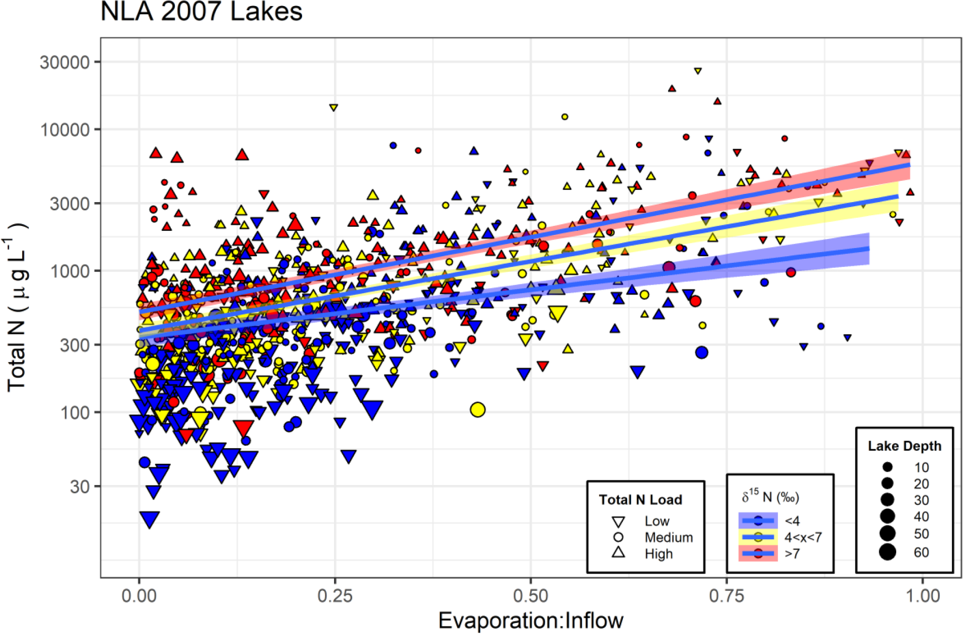
The relationship between total nitrogen concentration and the evaporation:inflow ratio (Brooks et al. 2014). Chironomid δ¹⁵N at each site is indicated by color with values lower than 4 ‰ in blue, values between 4 and 7 ‰ in yellow and values greater than 7 ‰ indicated in red. Thresholds are lower than for Figure 5 because median of NLA δ¹⁵N values was lower than for NRSA samples. Symbols represent represents total nitrogen inputs to the watershed (Low < 10 kg ha⁻¹ yr⁻¹, High > 50 kg ha⁻¹ yr⁻¹, and Medium are inputs between Low and High thresholds). Symbol size represents lake depth in meters.

3.3.2. Rivers and Streams

For NRSA rivers and streams in this study, N inputs to the landscape explained a much greater proportion of variation in [TN] than for NLA lakes (Table 3, Figure 5b). Nitrogen fertilizer applications within the watershed explained approximately 34 % of variation, while including the other forms of N increased that prediction power to 43 % of the variation. Including chironomid δ¹⁵N increased the predictive power to 39 % with fertilizer, and 48 % using all N sources. Nitrogen inputs and chironomid δ¹⁵N had a significant interaction (Table 3), where [TN] increased with chironomid δ¹⁵N values at low landscape N inputs, but at high levels of landscape N inputs, [TN] decreased with increasing chironomid δ¹⁵N values (Figure 5b). When landscape N inputs were below 10 kg ha⁻¹ yr⁻¹, median [TN] more than doubled from 170 to 523 μg L⁻¹ when chironomid δ¹⁵N values at the sites increased from < 5 to > 10 ‰. However, when landscape N inputs were above 100 kg ha⁻¹ yr⁻¹, median [TN] decreased by over 6-fold from 12,600 to 2,200 μg L⁻¹ when chironomid δ¹⁵N values at the sites increased from < 5 to > 10 ‰. The elevated δ¹⁵N values indicate that the large decrease in [TN] in the water with similarly high levels of N inputs was likely the result of nitrogen removal processes that fractionate against ¹⁵N such as denitrification and ammonia volatilization, leaving behind N enriched in ¹⁵N.

4. DISCUSSION

For national scale monitoring programs such as NARS, chironomid δ¹⁵N values provide useful information to help understand the possible N sources and watershed N transformation processes related to changes in [TN], particularly when combined with spatially extensive information on landscape N inputs (Sabo et al., 2019; Sobota et al., 2013). Chironomid δ¹⁵N values (Figure 2a,b) in over 2000 lakes, rivers, and streams across CONUS (Figure 1) were related to nitrogen inputs to the landscape, cycling of nitrogen which causes enrichment of ¹⁵N along the flowpath, and the resulting water chemistry in the water body. Very little of δ¹⁵N variation observed at this broad spatial scale was related to possible food-web dynamics (Figure 4), which was expected as we limited our sampling to chironomids - only one family of benthic insects - to minimize food-web related variance. Chironomids were ubiquitous across NARS sites and were an excellent taxon to use for monitoring δ¹⁵N across CONUS. For NLA 2007, lake properties were more important than landscape N inputs in explaining variation in lake [TN], likely because lake properties reflect internal N cycling and processing. However, by combining depth, E:I, total N inputs and chironomid δ¹⁵N, we could explain 61% of the variation in lake [TN]. For NRSA 2008–2009, total N inputs were the strongest driver of river and stream [TN] as previously found (Bellmore et al., 2018; Lin et al., 2021). However, chironomid δ¹⁵N values significantly improved this relationship by reflecting N processing and sources. Our data show that for watersheds with low nitrogen inputs, high chironomid δ¹⁵N values were associated with higher [TN], indicating that the N that reached rivers and streams was highly processed either as sources enriched in ¹⁵N such as manure or sewage, or through landscape level processing along the flowpath. On the other hand, when watersheds received high levels of nitrogen inputs, high chironomid δ¹⁵N values indicated a significant level of N removal processing and decreased [TN] in the waterway compared to locations with high inputs but low chironomid δ¹⁵N values. Identifying watersheds with high nitrogen removal processes could be very useful for understanding controls on these processes. In addition, identifying watersheds where high levels of N move into aquatic ecosystems with little or no processing (high input, high [TN], low δ¹⁵N) would also be useful for targeting nitrogen management or landscape engineering.

4.1. Objective 1: Drivers of Chironomid δ¹⁵N at the national scale

Chironomid δ¹⁵N values varied nearly 25 ‰ across the CONUS (Figure 1 and 2). This level of spatial variation is not unusual in aquatic organisms representing the basal part of the foodweb across large areas. Gu (2009) noted a similar level of δ¹⁵N variation in particulate organic matter (POM) in a review of approximately 100 lakes located around the globe. Jankowski et al. (2012) documented a 10 ‰ range of POM in 27 lakes within Washington state, and Vander Zanden et al. (2005) noted a 14 ‰ range in aquatic insects across 27 lakes in Denmark. Peipoch et al. (2012) found a range of 20 ‰ in basal resources of streams in their meta-analysis. A similar range was found in the synoptic survey by Diebel and Vander Zanden (2009) of aquatic insects in 72 streams across Wisconsin. In our study and these others, the sampling strategy was to avoid variation in δ¹⁵N related to trophic enrichment in ¹⁵N. While the chironomidae family does contain species in different feeding guilds, including some predator species that might influence δ¹⁵N, our random forest models indicated that feeding guilds including predators did not explain much variation in δ¹⁵N, particularly when compared with landscape or water chemistry parameters (Figure 4). In an unpublished study, we tested the difference between predator and non-predator chironomid taxa in sites across three river basins in Oregon, USA. Predators were on average 0.6 ‰ higher in δ¹⁵N from non-predator chironomids at the same site, but that difference was similar to the standard deviation between replicates of non-predator chironomids from the same location (0.5 ‰) (Brooks and Herlihy, unpublished data). While this trophic level variance likely contributes some noise in our data, it is not a significant source of variability relative to national or regional scale δ¹⁵N differences.

Across the NARS revisit sites, we found that the root mean squared error between δ¹⁵N values of chironomids collected independently from two different visits at the same site was 1.3 ‰ (noise), and the signal (variance between sites) was over 8 times larger than the noise (variance within a site). This consistency between groups of chironomids within a site indicates that site-level characteristics drove the variance in chironomid δ¹⁵N we observed across the survey sites (Kaufmann et al., 2014; Stoddard et al., 2008). This high level of spatial variation in chironomid δ¹⁵N across CONUS also highlights the importance of site-level measures of basal δ¹⁵N for foodweb studies using δ¹⁵N as an indicator of trophic level within an ecosystem (Casey and Post, 2011; Post, 2002).

4.1.1. Objective 2: Landscape drivers of Chironomid δ¹⁵N

Higher δ¹⁵N represents nitrogen that has been exposed to more nitrogen processing either through longer flowpaths (watershed size effect), slower movement (precipitation effect), and/or more microbial activity (temperature effect, nitrogen inputs). Microbial processes with the largest losses in ¹⁴N are those that cause gaseous loss of nitrogen (Denk et al., 2017), thus these nitrogen removal processes are contributing the most to elevated δ¹⁵N in the remaining N (Robinson, 2001). Chironomid δ¹⁵N values represent a mixture of nitrogen sources across the watershed. However, we found chironomid δ¹⁵N increased with increasing watershed size (Figure 3) indicating greater nitrogen cycling and microbial processing with longer flowpaths. Interestingly, [TN] did not change with watershed size (Figure 3), and neither did total N inputs to the landscape. Sources elevated in ¹⁵N (manure and sewage) slightly decreased with increasing watershed size, so the increases in chironomid δ¹⁵N with watershed size were not a result of increasing nitrogen inputs or mixing with N sources with elevated δ¹⁵N. The proportion of N that is transformed to gaseous N increases with longer residence time (Seitzinger et al., 2006), thus legacy N with long travel times into rivers and streams would be expected to have elevated δ¹⁵N. Nitrogen within soils has been found to increase in δ¹⁵N with residence time (Amundson et al., 2003), soil age (Vitousek et al., 1989) and potential to cycle N (Billy et al., 2010). While these studies investigated δ¹⁵N in soils, which are relatively stationary, the same trends should be true of δ¹⁵N in water: we expect nitrogen processing to occur along the flowpaths to aquatic ecosystems, with increased δ¹⁵N with longer flowpaths.

Riparian areas and hyporheic zones are well documented sites for N processing causing elevated δ¹⁵N in the remaining N entering aquatic systems (Hinkle et al., 2001; Ostrom et al., 2002; Wexler et al., 2011). In previous studies, both foliage of riparian plants (Hall et al., 2015) and nitrate (Wexler et al., 2012) increased in δ¹⁵N with increasing distance downstream. Thus, N traveling along longer flowpaths or having longer residence time would be expected to have greater δ¹⁵N, so the observed higher chironomid δ¹⁵N with increasing watershed size could indicate a greater proportion of older, legacy N entering aquatic systems in larger watersheds.

Climate factors also support the idea of longer residence time and more exposure to microbial activity along the flowpath causing the elevated δ¹⁵N found in chironomids. Greater precipitation lead to lower chironomid δ¹⁵N values in this study. The amount of precipitation influences the speed at which nitrogen travels along its flowpath, and the time for microbial activity. Faster movement with more precipitation would mean less exposure to N cycling and microbial processing. Warmer temperatures are associated with higher chironomid δ¹⁵N as well, likely indicating greater microbial activity in warmer climates. Indeed, global patterns of plant and soil δ¹⁵N show a similar pattern of increasing δ¹⁵N with decreasing precipitation and increasing temperatures which the authors attribute to microbial processing rates (Amundson et al., 2003; Austin and Vitousek, 1998; Craine et al., 2009; Craine et al., 2015).

Nitrogen inputs to the landscape are a primary control of N transformation processes such as denitrification and ammonia volatilization (Seitzinger et al., 2006; Yu et al., 2020); thus, this study and others have observed greater δ¹⁵N values in aquatic organisms with increasing human land-use activities that add nitrogen to the watersheds (Figures 4, Atkinson et al., 2014; Diebel and Vander Zanden, 2009; Peipoch et al., 2012; Vander Zanden et al., 2005). This pattern could be caused by the type of nitrogen being added (source δ¹⁵N values) and/or the cycling and processing of the nitrogen within the watershed as discussed above (Robinson, 2001). Manure and sewage are two common sources of nitrogen that have elevated δ¹⁵N values because they represent highly processed pools of nitrogen. In this study, the amount of manure and sewage added to the watershed ranked similarly to watershed area in explaining chironomid δ¹⁵N variation (Figure 4). However, Diebel and Vander Zanden (2009) found that the amount of manure applied to the watershed was a poor predictor of aquatic invertebrate δ¹⁵N in streams across Wisconsin, and instead found inorganic fertilizer and wetland area to be much better predictors. At the scale of CONUS, both N source and processing are likely important. Our interest is not in predicting chironomid δ¹⁵N values, but rather in using those values as a tool with other information to help understand this CONUS-scale variation in [TN] (See section 4.2 below).

4.1.2. Chironomid δ¹⁵N differences between lotic and lentic systems

While the range of δ¹⁵N values were similar between NLA and NRSA sites, NLA lakes had significantly lower chironomid δ¹⁵N values than the NRSA rivers and streams. This difference was partly explained because NLA lakes were skewed towards smaller watersheds compared to NRSA sites (Figure 3), but even after accounting for watershed size effects, lakes still had lower chironomid δ¹⁵N values by about 1 ‰. Nitrogen inputs did not cause the δ¹⁵N difference since NLA and NRSA watersheds did not systematically differ in N inputs (ANOVA, F=0.2, df=2027, p=0.66). We examined whether the largest N input source for sites varied between surveys and found the proportion of sites similarly distributed with both surveys having approximately 46% of sites with atmospheric deposition as the largest source, 33% with synthetic fertilizers, 2% with agricultural crop fixation, and 18% for manure and sewage. Two variables that were ranked as most important in the random forest models were [TN] and conductivity (Figure 4). Total [N] tended to be lower in NLA sites (ANOVA, F=6.42, df=2023, p=0.02), but conductivity was similar between the surveys (ANOVA, F=1.06, df=2023, p=0.3). We found lake [TN] was more driven by internal processes than rivers and streams [TN] (Table 2 and 3). Thus, within lake processes related to nitrogen cycling likely contributed to the difference in chironomid δ¹⁵N values between lakes and streams.

One factor in lakes that could lower δ¹⁵N values is N fixation from cyanobacteria (Gu, 2009). When lakes have a low N:P level (less than 15.3 based on mass), N fixation may be an important source of N (Jankowski et al., 2012). However, we found that NLA lakes with N:P mass based ratios lower than 15 had significantly higher δ¹⁵N values than those with higher N:P ratios (ANOVA, F=16.3, df=872, p < 0.001), so while nitrogen fixation may be happening in these lakes, other sources or processes are obscuring the N fixing isotopic signal. For example, Ginger et al. (2017) found that for a given level of total P in lakes, clear lakes had lower [TN] and higher δ¹⁵N values in seston than turbid lakes, which they attributed to higher rates of lake denitrification in clear lakes than in turbid lakes. We did not find any differences in NRSA chironomid δ¹⁵N values based on water N:P ratios (ANOVA, F=2.2, df=1080, p = 0.11). Thus, after accounting for basin size the pattern of higher chironomid δ¹⁵N in NRSA rivers and streams when compared to NLA lakes remains unexplained.

4.1.3. Water chemistry and chironomid δ¹⁵N

The most important variables in our random forest models explaining chironomid δ¹⁵N values were water chemistry variables (Figure 4) with conductivity the top ranked for lakes, and both [TN] and conductivity the top variables for rivers and streams. These variables remained the most important even after combining landscape, water body and potential food web variables into one random forest model (Figure 4). The strong tie between instantaneous measures of water chemistry and chironomid δ¹⁵N indicate that the nitrogen bound to organic matter is still strongly related to current cycling processes and reflects the solute concentrations within the water column. Thus, chironomid δ¹⁵N values can be useful tool in understanding nutrient pollution issues across broad spatial scales.

4.2. Objective 3: Chironomid δ¹⁵N as indicators of N processing and N pollution.

While many studies have linked increasing δ¹⁵N values of either nitrate or organic matter to increasing N inputs in broad scale surveys (Alam et al., 2020; Atkinson et al., 2014; Cabana and Rasmussen, 1996; Guiry, 2019; Morrissey et al., 2013; Peipoch et al., 2012), only one broad survey that we could find had linked the δ¹⁵N values to decreases in [TN] within the stream indicating denitrification (Diebel and Vander Zanden, 2009). Most studies linking δ¹⁵N and denitrification happen at the catchment scale in single study location with intensive sampling (Wexler et al., 2014; Wexler et al., 2011; Wexler et al., 2012). However, Diebel and Vander Zanden (2009) found that for high N inputs, high δ¹⁵N values were associated with lower nitrate concentrations in their survey of Wisconsin streams. Because of the large sample size in this study, we were able to detect a more complex interaction between chironomid δ¹⁵N and N inputs in explaining [TN] in lakes, rivers, and streams across the CONUS (Figure 5, Table 2, 3).

The N input – [TN] relationship in lakes was not as strong as for rivers and streams (Figure 5) because lakes were driven by both watershed and internal processes controlling lake [TN] (Table 2, Figure 6, Fraterrigo and Downing, 2008). Lake depth and E:I were more important than N inputs at explaining variation in lake [TN] (Table 2), but all were significant reflecting this balance between watershed and internal processes (Brooks et al., 2014; Read et al., 2015). When N inputs levels are low, the chironomid δ¹⁵N values indicated that the nitrogen associated with higher [TN] in lakes is more processed than that at lower lake concentrations, but this effect was diminished at high N inputs (Figure 5). Finlay et al. (2013) illustrated that if phosphorus was not limiting, then lake nitrogen removal processes increased with increasing N inputs, and likely explains our significant interaction between chironomid δ¹⁵N and N inputs (Table 2). Higher lake [TN] and chironomid δ¹⁵N were associated with higher temperatures and lower precipitation rates similar to global patterns of soil δ¹⁵N (Amundson et al., 2003), suggesting a link between higher N processing and N availability within lakes. While we clearly saw high δ¹⁵N values indicating high processing and likely N removal in lakes, we did not see a clear connection to lower [TN] in sites with high chironomid δ¹⁵N. The combined internal and watershed processes make interpretation of chironomid δ¹⁵N complicated in lakes, but when linked to lake morphological features (lake depth) and with hydrologic flows (E:I), δ¹⁵N was still useful for knowing which lakes have highly cycled N, particularly at the low end of N inputs (Figure 6).

Chironomid δ¹⁵N only clearly indicated N transformation processes that result in gaseous loss and significantly reduced [TN] at high levels in N inputs (>100 kg ha⁻¹ yr⁻¹) in rivers and streams (Figure 5). Above this nutrient input threshold, low chironomid δ¹⁵N values (<5 ‰) were associated with some of the highest measures of [TN] in NRSA sites, indicating nitrogen that moved rapidly through the watershed into the aquatic ecosystem with little to no nutrient processing. In the NSRA sites, chironomid δ¹⁵N greater than 10 ‰ were associated with [TN] six times lower than that with δ¹⁵N values below 5 ‰ indicating a high degree of gaseous N loss within those high δ¹⁵N watersheds. These high processing watersheds had a higher proportion of forested land and wetlands, and lower annual precipitation amounts as compared to watersheds where nitrogen quickly flushed into the stream. Others have found that the proportion of wetlands and forests within watersheds is associated with lower nitrogen levels found within streams at these broad spatial scales (e.g., Bellmore et al., 2018; Diebel and Vander Zanden, 2009; Lin et al., 2021). Incorporating chironomid δ¹⁵N data into these large-scale spatial analyses provides strong evidence that higher rates of denitrification were causing the observed reductions in [TN] at these high input levels.

At low levels of N inputs (<10 kg ha⁻¹ yr⁻¹), the pattern is reversed: higher δ¹⁵N values are associated with higher [TN] for both NRSA and NLA sites. Nearly 30% of sites in both NLA and NRSA (587 sites) had N inputs below 10 kg ha⁻¹ yr⁻¹. In these cases, higher δ¹⁵N could indicate sources of N elevated in ¹⁵N, such as manure or sewage, or older, highly processed legacy N entering the system, and not reflected in the recent N input data layers (Hu et al., 2019; Van Meter et al., 2016). For the low input NRSA sites, total N inputs still explained some variation in [TN]. Chironomid δ¹⁵N increased with increasing N inputs, but the nitrogen source (enriched or not in ¹⁵N) did not help explain the variation in either δ¹⁵N or [TN]. Watersheds with greater proportions of forested lands and higher annual precipitation had both lower [TN] and δ¹⁵N values. Interestingly at this low N input level, wetlands were associated with higher [TN], perhaps due to N export from wetlands, but did not impact chironomid δ¹⁵N values. Baseflow index, which is an indicator of groundwater inflow, was associated with lower [TN] and did not influence chironomid δ¹⁵N values, indicating groundwater was diluting the nitrogen in rivers and streams at these low input levels, and was not a source. These wetland and baseflow results were similar to what Lin et al. (2021) found for [TN] across all NRSA surveys. All of these observations support the idea that at low N input rates, higher [TN] found in streams was likely from unknown N sources elevated in δ¹⁵N such as manure or human waste, or legacy N that has been enriched in ¹⁵N over longer, slower flowpaths, but that groundwater was not the source of this N.

5. CONCLUSIONS

Chironomid δ¹⁵N values integrated watershed processes that influenced nitrogen cycling within aquatic ecosystems. For broad scale ecological monitoring programs such as the EPA’s NARS program, chironomid δ¹⁵N helped explain the variation in [TN], and was most useful in identifying rivers and streams with high gaseous N loss rates and thus high rates of N removal. Determining differences between watersheds that allow nitrogen to flow into streams unprocessed and those that transform N and lower [TN] for the same level of inputs could be highly useful for exploring potential mitigation strategies. At lower N input levels, the chironomid δ¹⁵N indicated that the source of N in lakes, rivers, and streams with high [TN] was a highly processed source not accounted for in the data layers, such as inputs of animal or human waste, or potentially older accumulated legacy N, but groundwater tended to dilute this unknown N source. Including chironomid δ¹⁵N in future surveys will help indicate how the prevalence of these processes are changing and the long-term implications for water quality. Since most broad scale surveys of water quality collect benthic macroinvertebrate samples to develop biological condition indexes, using subsamples of these samples for δ¹⁵N analysis can be inexpensive and relatively easy to conduct if the samples are preserved. Because chironomids are ubiquitous across lakes, rivers, and streams, focusing on their analysis is a good way to avoid most foodweb and trophic effects on δ¹⁵N, while ensuring broad distribution of sites and helps set a baseline of δ¹⁵N values in aquatic systems in the CONUS (Figure 1). The NARS surveys have found that the biological condition of approximately 25% of lakes, rivers and streams could be improved by decreasing [TN]; chironomid δ¹⁵N is one more tool to help understand the causes and possible sources of this pollution and can help indicate potential solutions.

Highlights.

• The δ¹⁵N of chironomids integrates nitrogen sources and processes across watersheds

• We measured chironomid δ¹⁵N in over 2000 locations across the USA

• With high N inputs, increasing chironomid δ¹⁵N indicated higher N removal processes

• With low N inputs, increasing chironomid δ¹⁵N indicated N sources enriched in ¹⁵N

• δ¹⁵N of chironomids helps inform national monitoring programs about N as a stressor

DATA AVAILABILITY

All NARS data from 2007–2009 is available at https://www.epa.gov/national-aquatic-resource-surveys/data-national-aquatic-resource-surveys Chironomid δ¹⁵N and δ¹³C data is available through EPA’s ScienceHub at DOI: 10.23719/1523163

REFERENCES

- Alam MK, Negishi JN, Rahman MATMT, Tolod JR. Stable isotope ratios of emergent adult aquatic insects can be used asindicators of water pollution in the hyporheic food web. Ecological Indicators 2020; 118: 106738. DOI: 10.1016/j.ecolind.2020.106738. [DOI] [Google Scholar]
- Amundson R, Austin AT, Schuur EAG, Yoo K, Matzek V, Kendall C, et al. Global patterns of the isotopic composition of soil and plant nitrogen. Global Biogeochemical Cycles 2003; 17. DOI: 10.1029/2002gb001903. [DOI] [Google Scholar]
- Atkinson CL, Christian AD, Spooner DE, Vaughn CC. Long-lived organisms provide an integrative footprint of agricultural land use. Ecological Applications 2014; 24: 375–384. DOI: 10.1890/13-0607.1. [DOI] [PubMed] [Google Scholar]
- Austin AT, Vitousek PM. Nutrient dynamics on a precipitation gradient in Hawai’i. Oecologia 1998; 113: 519–529. DOI: 10.1007/s004420050405. [DOI] [PubMed] [Google Scholar]
- Bai E, Houlton BZ, Wang YP. Isotopic identification of nitrogen hotspots across natural terrestrial ecosystems. Biogeosciences 2012; 9: 3287–3304. DOI: 10.5194/bg-9-3287-2012. [DOI] [Google Scholar]
- Baron JS, Driscoll CT, Stoddard JL, Richer EE. Empirical critical loads of atmospheric nitrogen deposition for nutrient enrichment and acidification of sensitive US Lakes. BioScience 2011; 61. DOI: 10.1525/bio.2011.61.8.6. [DOI] [Google Scholar]
- Bellmore RA, Compton JE, Brooks JR, Fox EW, Hill RA, Sobota DJ, et al. Relative importance of anthropogenic sources and internal sinks for nitrogen concentrations in U.S. streams and rivers. Science of the Total Environment 2018; 639: 1349–1359. DOI: 10.1016/j.scitotenv.2018.05.008. [DOI] [PMC free article] [PubMed] [Google Scholar]
- Billy C, Billen G, Sebilo M, Birgand F, Tournebize J. Nitrogen isotopic composition of leached nitrate and soil organic matter as an indicator of denitrification in a sloping drained agricultural plot and adjacent uncultivated riparian buffer strips. Soil Biology and Biochemistry 2010; 42: 108–117. DOI: 10.1016/j.soilbio.2009.09.026. [DOI] [Google Scholar]
- Boyer EW, Goodale C, Jaworski NA, Howarth RW. Anthropogenic nitrogen sources and relationships to riverine nitrogen export in the northeastern U.S.A. Biogeochemistry 2002; 57/58: 137–169. DOI: 10.1023/A:1015709302073. [DOI] [Google Scholar]
- Brooks JR, Gibson JJ, Birks SJ, Weber MH, Rodecap K, Stoddard JL. Stable Isotope estimates of lake water evaporation:inflow and residence time for lakes across the United States as a tool for national lake water quality assessments. Limnology and Oceanography 2014; 59: 2150–2165. DOI: 10.4319/lo.2014.59.6.2150. [DOI] [Google Scholar]
- Cabana G, Rasmussen JB. Comparison of aquatic food chains using nitrogen isotopes. Proceedings of the National Academy of Sciences 1996; 93: 10844–10847. DOI: 10.1073/pnas.93.20.10844. [DOI] [PMC free article] [PubMed] [Google Scholar]
- Camargo JA, Alonso A. Ecological and toxicological effects of inorganic nitrogen pollution in aquatic ecosystems: A global assessment. Environment International 2006; 32: 831–849. DOI: 10.1016/j.envint.2006.05.002. [DOI] [PubMed] [Google Scholar]
- Carpenter SR, Caraco NF, Correll DL, Howarth RW, Sharpley AN, Smith VH. Nonpoint pollution of surface waters with phosphorus and nitrogen. Ecological Applications 1998; 8: 559–568. DOI: 10.1890/1051-0761(1998)008[0559:NPOSWW]2.0.CO;2. [DOI] [Google Scholar]
- Casey MM, Post D. The problem of isotopic baseline: Reconstructing the diet and trophic position of fossil animals. Earth-Sceince Reviews 2011; 106: 131–148. DOI: 10.1016/j.earscirev.2011.02.001. [DOI] [Google Scholar]
- Craine JM, Elmore AJ, Aidar MPM, Bustamante M, Dawson JO, Hobbie EA, et al. Global patterns of foliar nitrogen isotopes and their relationships with climate, mycorrhizal fungi, foliar nutrient concentrations, and nitrogen availability. New Phytologist 2009; 183: 980–992. DOI: 10.1111/j.1469-8137.2009.02917.x. [DOI] [PubMed] [Google Scholar]
- Craine JM, Elmore AJ, Wang L, Augusto L, Baisden WT, Brookshire ENJ, et al. Convergence of soil nitrogen isotopes across global climate gradients. Scientific Reports 2015; 5: 8280. DOI: 10.1038/srep08280. [DOI] [PMC free article] [PubMed] [Google Scholar]
- Denk TRA, Mohn J, Decock C, Lewicka-Szczebak D, Harris E, Butterbach-Bahl K, et al. The nitrogen cycle: A review of isotope effects and isotope modeling approaches. Soil Biology and Biochemistry 2017; 105: 121–137. DOI: 10.1016/j.soilbio.2016.11.015. [DOI] [Google Scholar]
- Diebel MW, Vander Zanden MJ. Nitrogen stable isotopes in streams: effects of agricultural sources and transformations. Ecological Applications 2009; 19: 1127–1134. DOI: 10.1890/08-0327.1. [DOI] [PubMed] [Google Scholar]
- Dodds WK, Bouska WW, Eitzmann JL, Pilger TJ, Pitts KL, Riley AJ, et al. Eutrophication of U.S. freshwaters: analysis of potential economic damages. Environmental Science and Technology 2009; 43: 12–19. DOI: 10.1021/es801217q. [DOI] [PubMed] [Google Scholar]
- Finlay JC, Small GE, Sterner RW. Human influences on nitrogen removal in lakes. Science 2013; 342: 247–250. DOI: 10.1126/science.1242575. [DOI] [PubMed] [Google Scholar]
- Fraterrigo JM, Downing DJ. The influence of land use on lake nutrients varies with watershed transport capacity. Ecosystems 2008; 11: 1021–1034. DOI: 10.1007/s10021-008-9176-6. [DOI] [Google Scholar]
- Galloway JN, Aber JD, Erisman JW, Seitzinger S, Howarth RW, Cowling EB, et al. The nitrogen cascade. BioScience 2003; 53: 341–356. DOI: 10.1641/0006-3568(2003)053[0341:TNC]2.0.CO;2. [DOI] [Google Scholar]
- Ginger LJ, Kimmer KD, Herwig BR, Hanson M,A., Hobbs WO, Small GE, et al. Watershed vs. within-lake drivers of nitrogen: phosphorus dynamics in shallow lakes. Ecological Applications 2017; 27: 2155–2169. DOI: 10.1002/eap.1599. [DOI] [PubMed] [Google Scholar]
- Gu B Variations and controls of nitrogen stable isotopes in particulate organic matter of lakes. Oecologia 2009; 160: 421–431. DOI: 10.1007/s00442-009-1323-z. [DOI] [PubMed] [Google Scholar]
- Guiry E Complexities of Stable Carbon and Nitrogen Isotope Biogeochemistry in Ancient Freshwater Ecosystems: Implications for the Study of Past Subsistence and Environmental Change. Frontiers in Ecology and Evolution 2019; 7. DOI: 10.3389/fevo.2019.00313. [DOI] [Google Scholar]
- Hall SJ, Hale RL, Baker MA, Bowling DR, Ehleringer JR. Riparian plant isotopes reflect anthropogenic nitrogen perturbations: robust patterns across land use gradients. Ecosphere 2015; 6: 200. DOI: 10.1890/es15-00319.1. [DOI] [Google Scholar]
- Herlihy AT, Paulsen SG, Kentula ME, Magee T, Nahlik A, Lomnicky GA. Assessing the relative and attributable risk of stressors to wetland condition across the conterminous United States. Environmental Monitoring and Assessment 2019; 191: 320. DOI: 10.1007/s10661-019-7313-7. [DOI] [PMC free article] [PubMed] [Google Scholar]
- Hill RA, Weber MH, Debbout RM, Leibowitz SG, Olsen AR. The Lake-Catchment (LakeCat) Dataset: characterizing landscape features for lake basins within the conterminous USA. Freshwater Science 2018; 37: 208–221. DOI: 10.1086/697966. [DOI] [PMC free article] [PubMed] [Google Scholar]
- Hill RA, Weber MH, Leibowitz SG, Olsen AR, Thornburgh DA. The stream-catchment (STREAMCAT) dataset: a database of watershed metrics for the contermious United States. Journal of the American Water Resources Association 2016; 52: 120–128. DOI: 10.1111/1752-1688.12372. [DOI] [Google Scholar]
- Hinkle SR, Duff JH, Triska FJ, Laenen A, Gates EB, Bencala KE, et al. Linking hyporheic flow and nitrogen cycling near the Willamette River - a large river in Oregon, USA. Journal of Hydrology 2001; 244: 157–180. DOI: 10.1016/S0022-1694(01)00335-3. [DOI] [Google Scholar]
- Holtgrieve GW, Schindler DE, Hobbs WO, Leavitt PR, Ward EJ, Bunting L, et al. A Coherent Signature of Anthropogenic Nitrogen Deposition to Remote Watersheds of the Northern Hemisphere. Science 2011; 334: 1545–1548. DOI: 10.1126/science.1212267. [DOI] [PubMed] [Google Scholar]
- Houlton BZ, Bai E. Imprint of denitrifying bacteria on the global terrestrial biosphere. Proceedings of the National Academy of Sciences of the United States of America 2009; 106: 21713–21716. DOI: 10.1073/pnas.0912111106. [DOI] [PMC free article] [PubMed] [Google Scholar]
- Hu M, Liu Y, Zhang Y, Dahlgren RA, Chen D. Coupling stable isotopes and water chemistry to assess the role of hydrological and biogeochemical processes on riverine nitrogen sources. Water Research 2019; 150: 418–430. DOI: 10.1016/j.watres.2018.11.082. [DOI] [PubMed] [Google Scholar]
- Jankowski K, Schindler DE, Holtgrieve GW. Assessing nonpoint-source nitrogen loading and nitrogen fixation in lakes using δ15N and nutrient stoichiometry. Limnology and Oceanography 2012; 57: 671–683. DOI: 10.4319/lo.2012.57.3.0671. [DOI] [Google Scholar]
- Jordan SJ, Stoffer J, Nestlerode JA. Wetlands as sinks for reactive nitrogen at continental and global scales: A meta-analysis. Ecosystems 2011; 14: 144–155. DOI: 10.1007/s10021-010-9400-z. [DOI] [Google Scholar]
- Kaufmann PR, Hughes RM, Van Sickle J, Whittier TR, Seeliger CW, Paulsen SG. Lakeshore and littoral physical habitat structure: A field survey method and its precision. Lake and Reservoir Management 2014; 30: 157–176. DOI: 10.1080/10402381.2013.877543. [DOI] [Google Scholar]
- Kendall C, Elliott EM, Wankel SD. Tracing anthropogenic inputs of nitrogen to ecosystems. In: Michener R, Lajtha K, editors. Stable Isotopes in Ecology and Environmental Science. Wiley, 2007, pp. 375–449. [Google Scholar]
- Liaw A, Wiener M. Classification and Regression by randomForest., R News 2(3), 18–22., 2002. [Google Scholar]
- Lin J, Compton JE, Hill RA, Herlihy AT, Sabo R, Pickard B, et al. Context is everything: Interacting inputs and landscape characteristics control stream nitrogen. Environmental Science and Technology 2021; 55: 7890–7899. DOI: 10.1021/acs.est.0c07102. [DOI] [PMC free article] [PubMed] [Google Scholar]
- Mayer PM, Reynolds SK, McCutchen MD, Canfield TJ. Meta-Analysis of Nitrogen Removal in Riparian Buffers. journal of Environmental Quality 2007; 36: 1172–1180. DOI: 10.2134/jeq2006.0462. [DOI] [PubMed] [Google Scholar]
- Morrissey CA, Boldt A, Mapstone A, Newton J, Ormerod SJ. Stable isotopes as indicators of wastewater effects on the macroinvertebrates of urban rivers. Hydrobiologia 2013; 700: 231–244. DOI: 10.1007/s10750-012-1233-7. [DOI] [Google Scholar]
- Ostrom NE, Hedin LO, von Fischer JC, Robertson GP. Nitrogen transformations and NO3- removal at a soil-stream interface: a stable isotope approach. Ecological Applications 2002; 12: 2027–1043. DOI: 10.1890/1051-0761(2002)012[1027:NTANRA]2.0.CO;2. [DOI] [Google Scholar]
- Peck DV, Olsen AR, Weber MH, Paulsen SG, Peterson C, Holdsworth SM. Survey design and extent estimates for the National Lakes Assessment. Freshwater Science 2013; 32: 1231–1245. DOI: 10.1899/11-075.1. [DOI] [Google Scholar]
- Peipoch M, Marti E, Gacia E. Variability in δ15N natural abundance of basal resources in fluvial ecosystems: a meta-analysis. Freshwater Science 2012; 31: 1003–1015. DOI: 10.1899/11-157.1. [DOI] [Google Scholar]
- Post D Using stable isotopes to estimate trophic position: models, methods, and assumptions. Ecology 2002; 83: 703–718. DOI: 10.1890/0012-9658(2002)083[0703:USITET]2.0.CO;2. [DOI] [Google Scholar]
- R Core Team. R: A language and environment for statistical computing. R Foundation for Statistical Computing, Vienna, Austria, 2020. [Google Scholar]
- Read EK, Patil VP, Oliver SK, Hetherington AL, Brentrup JA, Zwart JA, et al. The importance of lake-specific characteristics for water quality across the continental United States. Ecological Applications 2015; 25: 943–955. DOI: 10.1890/14-0935.1.sm. [DOI] [PubMed] [Google Scholar]
- Robinson D δ15N as an integrator of the nitrogen cycle. Trends in Ecology and Evolution 2001; 16: 153–162. DOI: 10.1016/S0169-5347(00)02098-X. [DOI] [PubMed] [Google Scholar]
- Sabo RD, Clark CM, Bash J, Sobota DJ, Cooter E, Dobrowolski JP, et al. Decadal shift in nitrogen inputs and fluxes across the contiguous United States: 2002–2012. Journal of Geophysical Research Biogeosciences 2019; 124: 3104–3124. DOI: 10.1029/2019JG005110. [DOI] [Google Scholar]
- Seitzinger S, Harrison JA, Bohlke JK, Bouwman AF, Lowrance R, Peterson BJ, et al. Denitrification across landscapes and waterscapes: a synthesis. Ecological Applications 2006; 16: 2064–2090. DOI: 10.1890/1051-0761(2006)016[2064:dalawa]2.0.co;2. [DOI] [PubMed] [Google Scholar]
- Sobota DJ, Compton JE, Harrison JA. Reactive nitrogen inputs to US lands and waterways: how certain are we about sources and fluxes? Frontiers in Ecology and the Environment 2013; 11: 82–90. DOI: 10.1890/110216. [DOI] [Google Scholar]
- Sobota DJ, Compton JE, McCrackin ML, Singh S. Cost of reactive nitrogen release from human activities to the environment in the United States. Environmental Research Letters 2015; 10 025006. DOI: 10.1088/1748-9326/10/2/025006. [DOI] [Google Scholar]
- Stoddard JL, Herlihy AT, Peck DV, Hughes RM, Whittier TR, Tarquinio E. A process for creating multimetric indices for large-scale aquatic surveys. Journal of the North American Benthological Society 2008; 27: 878–891. DOI: 10.1899/08-053.1. [DOI] [Google Scholar]
- Swaney DP, Hong B, Ti C, Howarth RW, Humborg C. Net anthropogenic nitrogen inputs to watersheds and riverine N export to coastal waters: a brief overview. Current Opinion in Environmental Sustainability 2012; 4: 203–211. DOI: 10.1016/j.cosust.2012.03.004. [DOI] [Google Scholar]
- Syvaranta J, Vesala S, Rask M, Ruuhijarvi J, Jones RI. Evaluating the utility of stable isotope analyses of archived freshwater sample materials. Hydrobiologia 2008; 600: 121–130. DOI: 10.1007/s10750-007-9181-3. [DOI] [Google Scholar]
- U. S. Environmental Protection Agency. National Rivers and Streams Assessment 2008–2009 technical report. In: Development OoWOoRa, editor. EPA/841/R-16/008. Office of Water and Office of Research and Development, Washington, D.C., 2016a. [Google Scholar]
- U. S. Environmental Protection Agency. National rivers and streams assessment 2008–2009: A collaborative survey. EPA/841/R-16/007. Office of Water and Office of Research and Development, Washington, D.C., 2016b, pp. 131. [Google Scholar]
- U. S. Environmental Protection Agency. National rivers and streams assessment 2013–2014: A collaborative survey. EPA 841-R-19–001. Office of Water and Office of Research and Development, Washington, DC., 2020. [Google Scholar]
- U.S. Environmental Protection Agency. National Rivers and Streams Assessment: Field Operations Manual. EPA-841-B-07–009. Office of Water and Office of Research and Development, Washington, D.C., 2007a. [Google Scholar]
- U.S. Environmental Protection Agency. Survey of the Nation’s Lakes. Field Operations Manual. EPA 841-B-07- 004. Office of Water and Office of Research and Development, Washington, D.C., 2007b. [Google Scholar]
- U.S. Environmental Protection Agency. National lakes assessment: A collabotative survey of the nations’s lakes. EPA 841-R-09–001. Office of Water and Office of Research and Development, Washington, D.C., 2009, pp. 103. [Google Scholar]
- U.S. Environmental Protection Agency. National lakes assessment: Technical appendix data analysis approach. EPA-841-R-09–001a. U.S. Environmental Protection Agency, Office of Water and Office of Research and Development, Washington, DC, 2010, pp. 63. [Google Scholar]
- U.S. Environmental Protection Agency. National Lakes Assessment 2012: A Collaborative Survey of Lakes in the United States. EPA 841-R-16–113. Office of Water and Office of Research and Development, Washington, DC., 2016. [Google Scholar]
- Van Breemen N, Boyer EW, Goodale C, Jaworski NA, Paustian K, Seitzinger P, et al. Where did all the nitrogen go? Fate of nitrogen inputs to large watersheds in the northeastern U.S.A. Biogeochemistry 2002; 57/58: 267–293. DOI: 10.1023/A:1015775225913. [DOI] [Google Scholar]
- Van Grinsven HJM, Holland M, Jacobsen BH, Klimont Z, Sutton MA, Willems WJ. Costs and benefits of nitrogen for Europe and implications for mitigation. Environmental Science and Technology 2013; 47: 3571–3579. DOI: 10.1021/es303804g. [DOI] [PubMed] [Google Scholar]
- Van Meter KJ, Basu NB, Veenstra JJ, Burras CL. The nitrogen legacy: emerging evidence of nitrogen accumulation in anthropogenic landscapes. Environmental Research Letters 2016; 11: 035014. DOI: 10.1088/1748-9326/11/3/035014. [DOI] [Google Scholar]
- Vander Zanden MJ, Vadedoncoeur Y, Diebel MW, Jeppesen E. Primary consumer stable nitrogen isotopes as indicators of nutrient source. Environmental Science and Technology 2005; 39: 7509–7515. DOI: 10.1021/es050606t. [DOI] [PubMed] [Google Scholar]
- Vitousek PM, Shearer G, Kohl DH. Foliar 15N natural abundance in Hawaiian rainforest: patterns and possible mechanisms. Oecologia 1989; 78: 383–388. DOI: 10.1007/BF00379113. [DOI] [PubMed] [Google Scholar]
- Wexler SK, Goodale CL, McGuire KJ, Bailey SW, Groffman PM. Isotopic signals of summer denitrification in a northern hardwood forested catchment. Proceedings of the National Academy of Sciences of the United States of America 2014; 111: 16413–16418. DOI: 10.1073/pnas.1404321111. [DOI] [PMC free article] [PubMed] [Google Scholar]
- Wexler SK, Hiscock KM, Dennis PF. Catchment-scale quantification of hyporheic denitrification using an isotopic and solute flux approach. Environmental Science and Technology 2011; 45: 3967–3973. DOI: 10.1021/es104322q. [DOI] [PubMed] [Google Scholar]
- Wexler SK, Hiscock KM, Dennis PF. Microbial and hydrological influences on nitrate isotopic composition in an agricultural lowland catchment. Journal of Hydrology 2012; 468–469: 85–93. DOI: 10.1016/j.jhydrol.2012.08.018. [DOI] [Google Scholar]
- Yu L, Zheng T, Zheng X, Hao Y, Yuan R. Nitrate source apportionment in groundwater using Bayesian isotope mixing model based on nitrogen isotope fractionation. Science of the Total Environment 2020; 718: 137242. DOI: 10.1016/j.scitotenv.2020.137242. [DOI] [PubMed] [Google Scholar]
Associated Data
This section collects any data citations, data availability statements, or supplementary materials included in this article.
Data Availability Statement