Maximal reproduction number estimation and identification of transmission rate from the first inflection point of new infectious cases waves: COVID-19 outbreak example

Abstract

The dynamics of COVID-19 pandemic varies across countries and it is important for​ researchers to study different kind of phenomena observed at different stages of the waves during the epidemic period. Our interest in this paper is not to model what happened during the endemic state but during the epidemic state. We proposed a continuous formulation of a unique maximum reproduction number estimate with an assumption that the epidemic curve is in form of the Gaussian curve and then compare the model with the discrete form and the observed basic reproduction number during the contagiousness period considered. Furthermore, we estimated the transmission rate from identification of the first inflection point of a wave of the curve of daily new infectious cases using the Bernoulli S–I (Susceptible–Infected) equation. We applied this new method to the real data from Cameroon COVID-19 outbreak both at national and regional levels. High correlation was observed between the socio-economic parameters and epidemiology parameters at regional level in Cameroon. Also, the method was applied to the second wave COVID-19 outbreak for the world data which is a period the phenomena we are considering were observed. Lastly, it was observed that the models presented results correspond with the epidemic dynamics in Cameroon and World data. We recommend that it is important to study what happened during the growth inflection point as some countries data did not climax.

1. Introduction

In recent time it was discovered that the COVID-19 virus is still mutating, hence it is possible as we approach different seasons due to the movement of people from one place to another and increase in travels that the transmission rate from one person to the other may increase exponentially, but the aggressive vaccination campaign by policy makers, government introduction of lockdowns and some level of restriction in order to mitigate the virus spread may help to reduce the death rate. The United Kingdom health security agency reported on November 25, 2021 that a new COVID-19 variant that was first identified in Botswana is the most challenging variant yet and has doubled the number of mutations of Delta variant. The study of the spread of COVID-19 pandemic has been interest of researchers, most especially the socio-economic gap the situation has exposed in many countries.

Since the seminal article of D. Bernoulli in 1760 [1], and the improvements made by D. Ross [24], McKermack [17], and then by many other more recent authors [3], [4], [5], [14], [15], [16], [21], one of the central problems remains the estimate of the most important parameters of the equation governing the growth of observed infectious cases, namely the reproduction number each day during the contagious period of an infectious patient and the transmission rate.

In the first case, we propose a new method of estimating the maximum number of daily reproduction numbers and, in the second case, we describe a new method of calculating the rate of transmission by identifying the inflection points of the curve of new infectious cases observed.

In Section 2, we describe the method of estimating the maximum daily reproduction number, then in Section 3, the method of identifying inflection points of the curve of new infectious cases in the Bernoulli model. In Section 4, we apply these methods to data from the COVID-19 epidemic in Cameroon. Finally, in Section 5, we propose a generalization to other countries, in Section 6 a discussion, and eventually, we describe in Section 7 some perspectives of this work.

2. Maximal daily reproduction number estimation

Let us suppose that we consider an infectious disease outbreak in a country after a first random endemic period and fix the start of the epidemic wave at day $t_0$ when the number of the new cases ${{\mathrm{X}}_{\mathrm{t}}}_0$ has reached for the first time a threshold, for example equal to 100 new cases of infectious. We suppose that, if the duration of the infectivity (or contagiousness) period of an individual is equal to r days, we have recorded the new cases at times $t_0-1,\dots ,t_0$ − r. Then, for the days j $\ge$ $t_0$, we have:

$${\mathrm{X}}_{\mathrm{j}}={\sum }_{\mathrm{k=1,r}}{\mathrm{R}}_{\mathrm{k}}{\mathrm{X}}_{\mathrm{j-k}},$$ (1)

where the convolution equation (1) can be deconvolved in order to get the ${\mathrm{R}}_{\mathrm{k}}$’s, i.e., the numbers of people infected by an infectious individual during the kth day of his period of contagiousness [8]. ${\mathrm{R}}_{\mathrm{k}}$ is called the daily reproduction number at day k of the contagiousness period of an individual.

The deconvolution equation is given in matrix form by:

$$\mathrm{R}={\mathrm{M}}^{-1}\mathrm{X},$$ (2)

where X = (${\mathrm{X}}_{\mathrm{j}}$, …, ${\mathrm{X}}_{\mathrm{j-r-1}}$) is the vector of new infectious cases at days j, …, j − r ＋ 1 and R = (${\mathrm{R}}_1$, …, ${\mathrm{R}}_{\mathrm{r}}$) the vector of the daily reproduction numbers along the contagiousness period of length r. Both are r-dimensional vectors and M is defined as the following r–r matrix:

$$\mathrm{M}=\left(\begin{array}{cccc}\hfill {\mathrm{X}}_{\mathrm{j-1}}\hfill & \hfill {\mathrm{X}}_{\mathrm{j-2}}\hfill & \hfill \dots \hfill & \hfill {\mathrm{X}}_{\mathrm{j-r}}\hfill \\ \hfill \hfill & \hfill \hfill & \hfill \dots \hfill & \hfill \hfill \\ \hfill {\mathrm{X}}_{\mathrm{j-k-1}}\hfill & \hfill {\mathrm{X}}_{\mathrm{j-k-2}}\hfill & \hfill \dots \hfill & \hfill {\mathrm{X}}_{\mathrm{j-k-r}}\hfill \\ \hfill \hfill & \hfill \hfill & \hfill \dots \hfill & \hfill \hfill \\ \hfill {\mathrm{X}}_{\mathrm{j-r}}\hfill & \hfill {\mathrm{X}}_{\mathrm{j-r-1}}\hfill & \hfill \dots \hfill & \hfill {\mathrm{X}}_{\mathrm{j-2r+1}}\hfill \end{array}\right)$$ (3)

Remark

The number ${\mathrm{R}}_{\mathrm{j}}$ depends on the individual i and on the day j, and we would consider in fact the number ${\mathrm{R}}_{\mathrm{ikj}}$ of people infected at day j by a given infectious individual i during the kth day of his period of contagiousness of length ${\text{r}}_{\mathrm{i}}$. In the following, for the sake of simplicity, we neglect the dependency on i, j and r, which is reasonable during exponential growth [8].

2.1. Continuous observation time

Let us suppose that the observation time is continuous and that the new cases of infectious X(t) depend on the distribution of the quantities O(s) = R(s)/E(R), where the quantity E(R) = ${\int }_{\mathfrak{R}}$ R(t)dt:

$$\mathrm{X}\left(t\right)={\int }_{\mathfrak{R}}\mathrm{R}\left(\mathrm{s}\right)\mathrm{X}(t-\mathrm{s})d\mathrm{s}=E\left(\mathrm{R}\right){\int }_{\mathfrak{R}}\mathrm{X}(t-\mathrm{s})\mathrm{O}\left(\mathrm{s}\right)d\mathrm{s}$$ (4)

(a) we will suppose in a first case that the curve O(s) is a Gaussian curve $\mathcal{N}$(m, $\sigma$) then we have:

$$\mathrm{R}\left(\mathrm{s}\right)={\mathrm{R}}_{\max }exp(-{\left(\mathrm{s\; -\; m}\right)}^2/2{\sigma }^2),$$ (5)

where ${\mathrm{R}}_{\max }$ is the maximum of the daily reproduction numbers, and we will show that the continuous equivalent of Eq. (1) can be solved if X(t) is supposed to be exponential: X(t) $=$ 100 e${}^{\mathrm{ß}(\mathrm{t}-{\mathrm{t}}_0)}$ = c e${}^{\mathrm{ßt}}$, for t $\ge$ t₀, where $c=100$ e${}^{-\mathrm{ß}{\mathrm{t}}_0}$. Eq. (5) can be written as:

$$c{e}^{\mathrm{ßt}}={\int }_{\mathfrak{R}}{\mathrm{R}}_{\max }exp(-{(\mathrm{s}-\mathrm{m})}^2/2{\sigma }^2)c{e}^{\mathrm{ß(t-s)}}d\mathrm{s},$$

from which we deduce:

$$1={\mathrm{R}}_{\max }{\int }_{\mathfrak{R}}exp(-{(\mathrm{s}-\mathrm{m})}^2/2{\sigma }^2-ß\mathrm{s})d\mathrm{s}$$

$$1={\mathrm{R}}_{\max }{\int }_{\mathfrak{R}}exp(-{(\mathrm{s}-\mathrm{m}+ß{\sigma }^2)}^2/2{\sigma }^2+{ß}^2{\sigma }^2/2-ß\mathrm{m})d\mathrm{s}$$

$$1={\mathrm{R}}_{\max }\sigma {\left(2\pi \right)}^{\mathrm{1/2}}exp({ß}^2{\sigma }^2/2-ß\mathrm{m}){\int }_{\mathfrak{R}}exp(-{(\mathrm{s}-\mathrm{m}+ß{\sigma }^2)}^2/2{\sigma }^2)/\sigma {\left(2\pi \right)}^{\mathrm{1/2}}d\mathrm{s}$$

Hence, we obtain:

$$1={\mathrm{R}}_{\max }{\sigma \left(2\pi \right)}^{\mathrm{1/2}}exp({ß}^2{\sigma }^2/2-ß\mathrm{m})$$ (6)

and if we know $\sigma$ (4$\sigma$ $\approx$ r, the duration of the contagiousness period), m $\approx$ 2$\sigma$ and ß (the transmission rate), we get R${}_{\max }$, the value at day m (the middle of the contagiousness period) of the maximal daily reproduction number.

(b) if the curve of the daily reproduction numbers R(s) is the sum of two Gaussian-shaped curves, the first corresponding to the activation of the innate immunity and the second to the activation of the adaptive immunity, we have:

$$\mathrm{R}\left(\mathrm{s}\right)={\mathrm{R}}_{\mathrm{max1}}exp(-{(\mathrm{s}-{\mathrm{m}}_1)}^2/2{\sigma }_1^2)+{\mathrm{R}}_{\mathrm{max2}}exp(-{(\mathrm{s}-{\mathrm{m}}_2)}^2/2{\sigma }_2^2)$$

In this case, Eq. (5) can be written as:

$$c{e}^{\mathrm{ßt}}=[{\int }_{\mathfrak{R}}{\mathrm{R}}_{\mathrm{max1}}exp(-{(\mathrm{s}-{\mathrm{m}}_1)}^2/2{\sigma }_1^2)+{\mathrm{R}}_{\mathrm{max2}}exp(-{(\mathrm{s}-{\mathrm{m}}_2)}^2/2{\sigma }_2^2)]c{e}^{\mathrm{ß(t-s)}}d\mathrm{s}$$ (7)

Then, we obtain:

$$1={\mathrm{R}}_{\mathrm{max1}}exp({ß}^2{\sigma }_1^2/2-ß{\mathrm{m}}_1)+{\mathrm{R}}_{\mathrm{max2}}exp({ß}^2{\sigma }_2^2/2-ß{\mathrm{m}}_2)$$ (8)

formula from which we can calculate the value of a parameter in function of the value of others. If 4${\sigma }_1$ + 4${\sigma }_2$ can be estimated by the duration of the contagiousness period and if we suppose that ${\sigma }_1$ is close to ${\sigma }_2$, with ${\mathrm{m}}_1=2{\sigma }_1$ and ${\mathrm{m}}_2=4{\sigma }_1$ + 2${\sigma }_2$, then the only remaining unknown parameters are ${\mathrm{R}}_{\mathrm{max1}}$ and R_max2. If these two maximal daily reproduction numbers are supposed to be close, the Eq. (8) allows the final calculation of a unique ${\mathrm{R}}_{\max }$, which could be compared to the one obtained by the discrete method of deconvolution presented in [8].

2.2. Discrete observation time

(1) If the observation time is discrete, we replace O(s)=R(s)/E(R), with E(R) = ${\int }_{\mathfrak{R}}$ R(t)dt by O${}_{\mathrm{k}}$ = R${}_{\mathrm{k}}$/E(R), with E(R) = ${\sum }_{\mathrm{k=1,r}}$R${}_{\mathrm{k}}$ = R₀, where R₀ is the basic reproduction number and using Eq. (1), the Eq. (4) by:

$${\mathrm{X}}_{\mathrm{j}}={\sum }_{\mathrm{k=1,r}}{\mathrm{R}}_{\mathrm{k}}{\mathrm{X}}_{\mathrm{j-k}}\mathrm{X}\left(t\right)=\mathrm{E}\left(\mathrm{R}\right){\sum }_{\mathrm{k=1,r}}{\mathrm{X}}_{\mathrm{j-k}}{\mathrm{O}}_{\mathrm{k}},$$

where the distribution {O${}_{\mathrm{k}}$}${}_{\mathrm{k=1,r}}$ can have several uni- or bi-modal shapes estimated by deconvoluting Eq. (1) [8].

3. Estimation of transmission rate from identification of the first inflection point of a wave of the curve of daily new infectious cases

Following the same approach as in [9], we want now to derive the inflection point during the outbreak of COVID-19 pandemic using Bernoulli equation and to analyze this Susceptible–Infected​ (SI) compartment model for calculating the time of the inflection point of the curve of new infectious cases. First, let us recall that the SI Bernoulli differential equation model of an outbreak epidemic is given as:

$$\frac{dS}{dt}=-\frac{\beta }{S_o}S\left(t\right)I\left(t\right)+dS\left(t\right),\frac{dI}{dt}=\frac{\beta }{S_o}S\left(t\right)I\left(t\right)-\nu I\left(t\right),$$ (9)

where d is the susceptible demographic balance, $\nu$ the specific mortality rate due to the disease, $\beta /S_o$ the disease transmission rate, $S\left(t\right)$ the number of susceptible individuals, $I\left(t\right)$ the number of infectious individuals at time $t\ge 0$, and the initial conditions of the model are: $S\left(0\right)=S_o>0$ and $I\left(0\right)=1$.

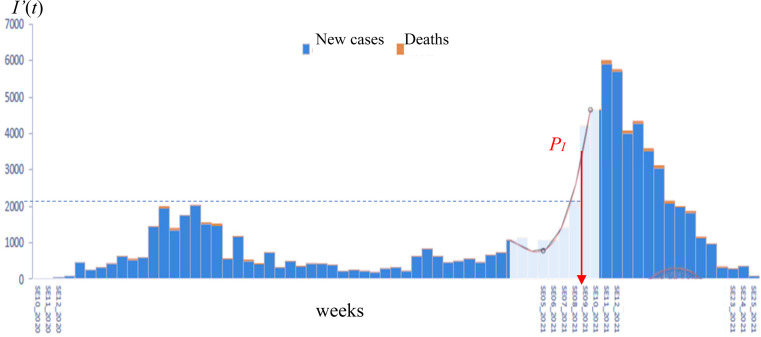
Graphical representation of the inflection point $P_I$ of the curve of $I^{\prime }\left(t\right)$ is given Fig. 1, for the first half part of the second wave of the COVID-19 weekly new reported cases between week 5 2021 and week 12 2021 (data from [2]). The red curve represents the cubic spline approximation of the raw data with the following statistics: $p$-value $=$ 0.03, Multiple R-squared MR $=$ 0.90, Relative Mean Square Error RMSE $=$ 0.247.

Fig. 1.

COVID-19 weekly new cases in Cameroon showing the inflection point $P_I$ (red arrow) during the first half part of the second wave between week 5 of 2021 and week 12 of 2021.

From [2].

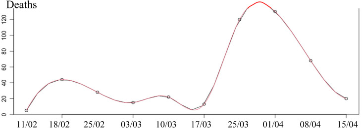
During the same period, it is also possible to smooth the death data (from [25]) with a cubic spline with the following statistics: $p$-value $=$ 0.12, Multiple R-squared MR $=$ 0.99, Relative Mean Square Error RMSE $=$ 4.380.

3.1. Mathematical formulation

We want to formulate the problem in such a way that we can identify all parameters from the set $0̸=\left\{(S_o,I_o,K,\beta )\right\}\subset {(0,\infty )}^4$ if we know the reported daily infectious cases $I^{\prime }\left(t\right)$ for all times $t\ge 0$. It should be noted that it is not sufficient alone to know the value of $I^{\prime }\left(t\right)$ at any time $t\ge 0$, because the knowledge about the value of $S_o$, the number of susceptible people in the population before the epidemic outbreak is also necessary to allow to obtain a precise information about the values of $I_o,K,\beta$ (see [6], [8], [9]).

Let usconsider the solution of the Bernoulli equation with d = $\nu =0$ (fertility and mortality rates negligible):

$$I\left(t\right)=\frac{S_o{e}^{\beta (t-a)}}{1+e^{\beta (t-a)}},S\left(t\right)=\frac{S_o}{1+e^{\beta (t-a)}},$$

where $S_0$, $\beta$ and a represent respectively the susceptible size at endemic start, transmission rate and endemic start time.

For any time t, we have:

$$I\left(t\right)+S\left(t\right)=S_o\left[\frac{e^{\beta (t-a)}}{1+e^{\beta (t-a)}}+\frac{1}{1+e^{\beta (t-a)}}\right]=S_o{e}^{\beta \left(t-a\right)}=\frac{I\left(t\right)}{S_o-I\left(t\right)}$$

If we consider that the epidemic wave starts at time 0, where I(0) $=$ 1, we have:

$$1=\frac{S_o{e}^{-\beta a}}{1+e^{-\beta a}}$$

Then, S(0) $=S_o$ – 1 and a is given by the following equation:

$$a=log(S_o-1)/\beta$$ (10)

3.2. Derivation of the equation of the inflection point $P_I$

From Bernoulli equation, where $\nu =0$; we have:

$$I^{\prime }\left(t\right)=\frac{dI}{dt}=\frac{\beta }{S_o}SI=\frac{\beta }{S_o}\times \frac{S_o}{1+e^{\beta (t-a)}}\times \frac{S_o{e}^{\beta (t-a)}}{1+e^{\beta (t-a)}}=\frac{\beta S_o{e}^{\beta (t-a)}}{{(1+e^{\beta (t-a)})}^2}$$

The sufficient existence condition for a point of inflection of order 2 for $I^{\prime }\left(t\right)$ in the case that $I\left(t\right)$ is 3-times continuously differentiable in a certain neighborhood of a point $t_i$, with $I^{‴}\left(t_i\right)=0$, and $I^{″}\left(t_i\right)\ne 0$. Then, $I^{\prime }\left(t\right)$ has an inflection point ($P_I$) of order 2 at $t_i,\text{ and by }$ differentiating $I^{\prime }\left(t\right)$ twice, we get:

$$I^{\prime \prime }\left(t\right)=\frac{d^{2}I}{d{t}^2}={\beta }^2{S}_o\frac{e^{\beta (t-a)}-2e^{2\beta (t-a)}}{{(1+e^{\beta (t-a)})}^3}$$

$$I^{\prime \prime \prime }\left(t\right)=\frac{d^{3}I}{d{t}^3}={\beta }^3{S}_o\frac{e^{\beta (t-a)}(1-6e^{\beta (t-a)}+2e^{2\beta (t-a)})}{{(1+e^{\beta (t-a)})}^4}$$

Then, the equation giving $\beta$ and a from its lowest root $x_i=3-\sqrt{7}=e^{\beta \left(t_i-a\right)}=\frac{I\left(t_i\right)}{S_o-I\left(t_i\right)}$ (depending on $I\left(t_i\right))$ is:

$$1-6x_i+2x_i^2=1-6e^{\beta \left(t_i-a\right)}+2e^{2\beta \left(t_i-a\right)}=0$$ (11)

If we assume now $I\left(0\right)=100$, then from the same calculations, we can identify the values of $\beta$ and a from the Eqs. (10), (11).

3.3. Identification method

If we calculate the value of the time $t_i$at which the first $P_I$ of a wave is observed and if we know the value of $S_0$, then we can estimate the maximal reproduction number as $I^{\prime \prime }\left(t_i\right)$ and identify $\beta$ and a from the Eqs. (10), (11). The steps of the identification method are as follows:

• 1.From an interpolation of the curve of the daily reported new cases (see for example red curve in Fig. 1) of a particular country epidemic wave, we calculate the lowest $t_i$ of the wave at which $I^{‴}\left(t_i\right)=0$,
• 2.From the value of $t_i$, we estimate the maximal reproduction number as $I^{\prime \prime }\left(t_i\right)$,
• 3.From the knowledge of S(0), the number of susceptible people in the population at the start of a particular country epidemic wave, we can get $S_o$,
• 4.From Eqs. (10), (11), we can identify $\beta \text{ and }a$.

4. Application to the COVID-19 outbreak in Cameroon

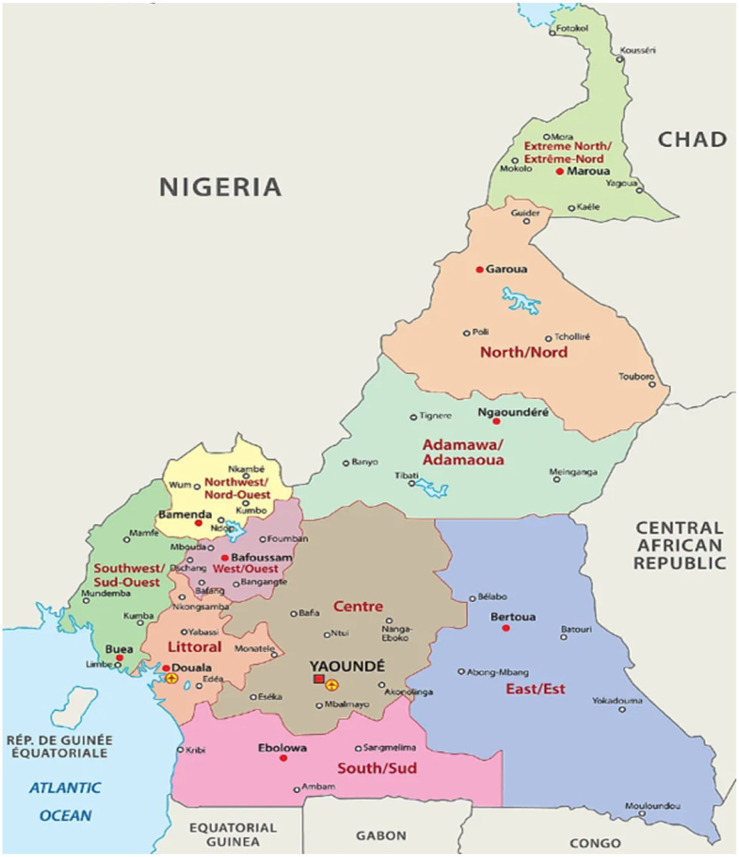
We will use in the following the Cameroon’s data concerning the COVID-19 outbreak and from the Cameroon Situation Reports (weekly regional new cases and deaths [2]) and from the public database Worldometers (weekly national new cases and deaths [25]). We will analyze in the following the Cameroon data at national and regional levels (see Fig. 3), by comparing the 10 regions from a set of socio-economic and epidemiologic variables (Table 3) whose data are coming from the public database of Globaldatalab [11].

Fig. 3.

The 10 regions of Cameroon.

From [25].

4.1. Estimation of the maximal basic reproduction number ${\mathrm{R}}_{0max}$ and of the maximal daily reproduction number ${\mathrm{R}}_{max}$

4.1.1. Study in Cameroon

(1) We first calculate the time $t_i$ of the first inflection point $P_I$ of the second wave of the new infectious cases X(t) for the Cameroon. For that, we have smoothed the raw data of the weekly reported new infectious cases in Fig. 2 by using a cubic spline and the maximal reproduction number is estimated by the maximal value of its slope divided by X(t) at t = t ${}_i=4$ (weeks), equal to ${\mathrm{R}}_{0_{\max }}=2.04$, close to the maximal value of the effective reproduction number given for this period by the public database Renkulab [23].

Fig. 2.

Spline graph for COVID-19 deaths in Cameroon during the second wave between week 5 of 2021 and week 14 of 2021.

(2) From Eq. (6), we can estimate the maximal daily reproduction number ${\mathrm{R}}_{\max }$:

$$1={\mathrm{R}}_{\max }\sigma {\left(2\pi \right)}^{\mathrm{1/2}}exp({ß}^2{\sigma }^2/2-ß\mathrm{m}),$$

Then, from [19] we estimate $\sigma =1$, m = 2, ß= $\beta /S_o=0.4$. Then, we have:

$${\mathrm{R}}_{\max }=1/{\left(2\pi \right)}^{\mathrm{1/2}}exp(0.8-0.08)\approx 0.9,$$

which corresponds in case of a Gaussian shape for the daily reproduction numbers ${\mathrm{R}}_{\mathrm{j}}$’s along the contagiousness period of length r $\approx$ 4$\sigma$ to a basic reproduction number ${\mathrm{R}}_0={\Sigma }_{\mathrm{k=1,r}}$R${}_{\mathrm{k}}$ $\approx$ 2.1.

4.1.2. Calculation of the distribution of daily reproduction numbers at the beginning of the pandemic in Cameroon

The numbers of new cases during the first wave between March 15 and March 28 2020 are the following:

$$\mathbf{March15}1,1,5,3,0,14,13,0,16,10,9,0,16,0\mathbf{March28}$$

Then, the matrix M defined in Section 2 is equal to:

$$\mathrm{M}=\left[\begin{array}{ccccccc}\hfill 16\hfill & \hfill 0\hfill & \hfill 9\hfill & \hfill 10\hfill & \hfill 16\hfill & \hfill 0\hfill & \hfill 13\hfill \\ \hfill 0\hfill & \hfill 9\hfill & \hfill 10\hfill & \hfill 16\hfill & \hfill 0\hfill & \hfill 13\hfill & \hfill 14\hfill \\ \hfill 9\hfill & \hfill 10\hfill & \hfill 16\hfill & \hfill 0\hfill & \hfill 13\hfill & \hfill 14\hfill & \hfill 0\hfill \\ \hfill 10\hfill & \hfill 16\hfill & \hfill 0\hfill & \hfill 13\hfill & \hfill 14\hfill & \hfill 0\hfill & \hfill 3\hfill \\ \hfill 16\hfill & \hfill 0\hfill & \hfill 13\hfill & \hfill 14\hfill & \hfill 0\hfill & \hfill 3\hfill & \hfill 5\hfill \\ \hfill 0\hfill & \hfill 13\hfill & \hfill 14\hfill & \hfill 0\hfill & \hfill 3\hfill & \hfill 5\hfill & \hfill 1\hfill \\ \hfill 13\hfill & \hfill 14\hfill & \hfill 0\hfill & \hfill 3\hfill & \hfill 5\hfill & \hfill 1\hfill & \hfill 1\hfill \end{array}\right]$$

and we have:

$${\mathrm{M}}^{-1}=\left[\begin{array}{ccccccc}\hfill 0.00582788\hfill & \hfill -0.00882952\hfill & \hfill 0.009303\hfill & \hfill -0.03084686\hfill & \hfill 0.0216235\hfill & \hfill -0.02815066\hfill & \hfill 0.06042457\hfill \\ \hfill -0.00882952\hfill & \hfill 0.0070809\hfill & \hfill -0.019324\hfill & \hfill 0.00609393\hfill & \hfill -0.01580307\hfill & \hfill 0.03737718\hfill & \hfill 0.03900754\hfill \\ \hfill 0.009303\hfill & \hfill -0.019324\hfill & \hfill -0.00781664\hfill & \hfill -0.00403656\hfill & \hfill 0.02691476\hfill & \hfill 0.06319195\hfill & \hfill -0.03605914\hfill \\ \hfill -0.03084686\hfill & \hfill 0.00609393\hfill & \hfill -0.00403656\hfill & \hfill 0.06311531\hfill & \hfill 0.04014842\hfill & \hfill -0.01719015\hfill & \hfill -0.05720378\hfill \\ \hfill 0.0216235\hfill & \hfill -0.01580307\hfill & \hfill 0.02691476\hfill & \hfill 0.04014842\hfill & \hfill -0.02492553\hfill & \hfill -0.01022751\hfill & \hfill -0.04545266\hfill \\ \hfill -0.02815066\hfill & \hfill 0.03737718\hfill & \hfill 0.06319195\hfill & \hfill -0.01719015\hfill & \hfill -0.01022751\hfill & \hfill -0.07132353\hfill & \hfill 0.01670959\hfill \\ \hfill 0.06042457\hfill & \hfill 0.03900754\hfill & \hfill -0.03605914\hfill & \hfill -0.05720378\hfill & \hfill 0.04545266\hfill & \hfill 0.01670959\hfill & \hfill 0.05053995\hfill \end{array}\right]$$

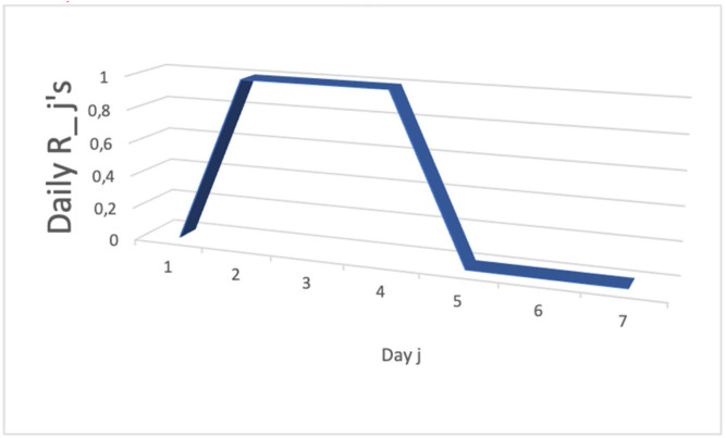
Because the vector of new infectious cases X = $\left[\begin{array}{c}\hfill 0\hfill \\ \hfill 16\hfill \\ \hfill 0\hfill \\ \hfill 9\hfill \\ \hfill 10\hfill \\ \hfill 16\hfill \\ \hfill 0\hfill \end{array}\right]$, hence R $=$ M⁻¹X = $\left[\begin{array}{c}\hfill -0.65306968\hfill \\ \hfill 0.60814399\hfill \\ \hfill 0.93470577\hfill \\ \hfill 0.7919826\hfill \\ \hfill -0.30440867\hfill \\ \hfill -0.80012803\hfill \\ \hfill -0.07788649\hfill \end{array}\right]$ and we can represent the evolution of the daily reproduction numbers R${}_{\mathrm{j}}$’s in​ Fig. 4, which shows a unimodal distribution on the first days (j = 1, …,4) of the infection period, with a sum of the R${}_{\mathrm{j}}$’s equal to 0.4, close to the effective reproduction number R${}_{\mathrm{e}}$ in [23].

Fig. 4.

The distribution of the daily reproduction numbers R${}_{\mathrm{j}}$’s on the infection period.

4.1.3. Study in other countries

We calculated the ${\mathrm{R}}_{\max }$ using same procedure as above for six other countries using the transmission rate of the first wave in 2020: Australia = 4.6214 $\times$ $10^{-8}$, Italy $=$ 1.2292 $\times$ $10^{-8}$, Spain $=$ 3.3182 $\times$ $10^{-7}$, United State $=$ 3.1828 $\times$ $10^{-7}$, United Kingdom $=$ 1.1526 $\times$ $10^{-7}$ and Canada = 2.0731 $\times$ $10^{-7}$) given in [22], with $\sigma =1$ and $\sigma =2$, corresponding to a duration of the contagiousness period of respectively 4 and 8 days. We also calculated ${\mathrm{R}}_{\mathrm{max2}}$ by using Eq. (8) presented in Table 2. We used the values of ${\mathrm{R}}_{\max }$ in Table 1 as ${\mathrm{R}}_{\mathrm{max1}}$ while still maintaining the values for the transmission rate and $\sigma$.

Table 2.

Result for R${}_{\mathrm{max2}}$ while using R${}_{\max }$ in Table 1 as R${}_{\mathrm{max1}}$ for different countries.

Countries	$\sigma$ = 2	$\sigma$ = 1
United Kingdom	0.79842	0.59769
Australia	0.79742	0.59608
Italy	0.79970	0.59974
Spain	0.79440	0.59129
Canada	0.79673	0.59498
United States	0.79466	0.59169

Table 1.

Result for R${}_{\max }$ for different countries.

Countries	$\sigma$ = 1	$\sigma$ = 2
United Kingdom	0.39978	0.20031
Australia	0.40018	0.20071
Italy	0.39927	0.19980
Spain	0.40136	0.20190
Canada	0.40018	0.20098
United States	0.40126	0.20180

4.2. Identification of the parameters $\beta \text{ and }a$

From Eqs. (10), (11), we get:

$$a=\text{Log}(S_o-1)/\beta \text{ and }1-6e^{\beta \left(t_i-a\right)}+2e^{2\beta \left(t_i-a\right)}=0,$$

with $S_o=27,000,000$ and $t_i=4$. Then $a=7$/$\beta$ and $1-6e^{4\beta -7}+2e^{8\beta -14}=0$, from which we get: $\beta =2.0$ and $a=3.5$, what is consistent for a with the previous estimation of $t_i$, but overvalued for $\beta$, perhaps due to an overestimation of $S_o$. Indeed, if $S_o$ corresponds to the population of the 3 regions (Littoral, Center and Northwest) giving the essential of the infectious cases (for example, 325/371 $=$ 88% of all the new cases during the week of 23/06/2021). More, if we consider the cumulative number of infectious during the whole week 8 of 2021, there was 2000 cases. If we consider that the susceptible population in contact with these infectious is 2000 $\times$ 50 $=$ 100,000, then from Eq. (10) $a=11.5$/$\beta$, and from Eq. (11), $\beta =2.4$ and $a=4.7$, which shows the sensitivity of calculation of $\beta$ to initial conditions concerning the susceptible population.

4.3. Study at the regional level

4.3.1. Estimation of the epidemiologic parameters

By using the methods proposed in Section 3, we obtain the value of the main epidemiologic parameters for each region of Cameroon (Table 3) and we observe a big difference between the urban regions, essentially the regions of Yaoundé and Douala (i.e. respectively the Center and Littoral regions) whose urban density is high and the other mainly rural regions.

Table 3.

Values of epidemiologic parameters for different regions of Cameroon.

Cameroon regions	Discrete R	Transmission rate $\beta$	R${}_{\max }$$\sigma =1$	R${}_{\max }$$\sigma =2$
Adamaoua	1.30175	1.50	2.60143	0.89396
Center	1.04135	1.75	2.85711	0.47851
Est	2.18015	1.50	2.60143	0.89396
Extreme_Nord	1.74880	1.50	2.60143	0.89396
Littoral	0.91404	1.75	2.85711	0.47851
Nord	1.31392	1.50	2.60143	0.89396
Nord_Ouest	3.64468	1.50	2.60143	0.89396
Ouest	3.38611	1.50	2.60143	0.89396
Sud	1.19674	1.50	2.60143	0.89396
Sud_Ouest	0.88279	1.50	2.60143	0.89396

4.3.2. Correlations between epidemiologic, socio-economic and demographic parameters

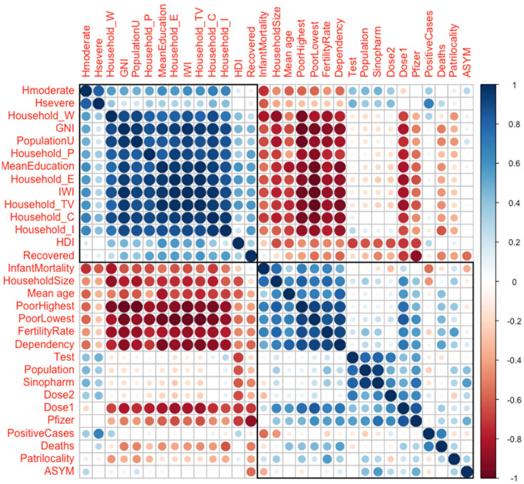
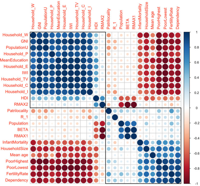
We have observed the epidemiologic variables (numbers of weekly reported new infectious cases, cured and deceased patients) during the 19 first weeks of 2021 (cf. in Fig. 1, data from [25]). The parameters list is given in Table 4 and their values are extracted from Table 3 and from [11], [23]. The correlations between the parameters of Table 1 considered as variables on the 10 regions of Cameroon can be analyzed thanks to Fig. 5, Fig. 6, which show that the epidemiologic parameters (from parameter Dose 1 to parameter Recovered) are significantly anti-correlated (pink color) with many socio-economic and demographic parameters, namely the three first ones (Subnational Human Development Index, International Wealth Index and Gross National Income per capita) and to those linked to the house holding, showing the influence of a good socio-economic state on the resistance against the virus.

Table 4.

List of the parameters considered for the different regions of Cameroon.

Socio-economic parameters
HDI	Subnational Human Development Index
IWI	International Wealth Index
GNI	Gross National Income per capita
PoorHighest	Percentage poor households (IWI value under 70)
PoorLowest	Percentage poor households (IWI value under 35)
MeanEducation	Mean years education population aged 20+
Household_TV	Percentage households with a TV
Household_C	Percentage households with a computer
Household_W	Percentage households with piped water
Household_E	Percentage households with electricity
Household_P	Percentage households with a phone
Household_I	Percentage households with internet access
HouseholdSize	Average household size
Patrilocality	Patrilocality index (positive values patrilocal)
Dependency	Dependency ratio
Demographic parameters
FertilityRate	Total fertility rate
InfantMortality	Infant mortality rate
Population	Total area population in millions
PopulationU	Urban population size
Epidemiologic parameters
Dose1	Number of vaccinated people that have received first dose
Dose2	Number of vaccinated people having received second dose
Pfizer	Number of vaccinated people with Pfizer vaccine
Sinopharm	Number of vaccinated people with Sinopharm vaccine
Test	Number of tested people
PositiveCases	Number of people that tested positive
ASYM	Patients that are asymptomatic and mild symptoms
Hmoderate	Patients with moderate symptoms
Hsevere	Patients with severe symptoms
Deaths	Number of deaths recorded
Recovered	Number of recovery recorded
R_1	Daily reproduction number of the first day of infection
Rmax1	R maximum first wave
Rmax2	R maximum second wave
BETA	Transmission rate

Fig. 5.

Correlations between various epidemiologic, socio-economic and demographic parameters observed in the different regions of Cameroon during the second wave. The false color scale indicates the intensity of the correlation between −1 and 1. (For interpretation of the references to color in this figure legend, the reader is referred to the web version of this article.)

Fig. 6.

Correlations between various epidemiologic, socio-economic and demographic parameters observed in the different regions of Cameroon during the second wave. The false color scale indicates the intensity of the correlation between −1 and 1. (For interpretation of the references to color in this figure legend, the reader is referred to the web version of this article.)

By exploiting the data corresponding to the parameters of Table 4, we can analyze the correlations existing between three families of parameters observed in the different regions of Cameroon during the second wave of the COVID-19 outbreak. In Fig. 5, we see that the socio-economic factors are highly positively correlated with each other, but negatively correlated with demographic parameters and not​ correlated with epidemiologic parameters, except those corresponding to vaccination and death which are anticorrelated with the signs of wealth. This can be explained by a higher socio-cultural level, which pushes individuals to monitor their health more and to get vaccinated. In Fig. 6, we can observe a greater number of demographic parameters that are anti-correlated with socio-economic factors. These are in particular infant mortality, mean age, fertility and poverty indicators, which have positive or zero correlation coefficients between them and very negative with wealth indicators, such as GNI or possession of material goods or land (television and house), because in general a rise in the standard of living causes fertility and infant mortality decrease.

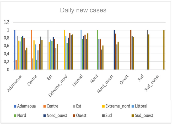
We observe in Fig. 7 a high correlation between Sud-Ouest and Littoral with the score 0.918 and the least correlations are between Center and Adamaoua with the score 0.242, between Est and Center with the score 0.282 and between Nord and Center with the score 0.253.

Fig. 7.

Correlations of the new cases numbers between the 10 regions of Cameroon.

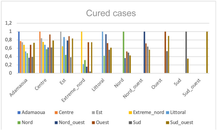
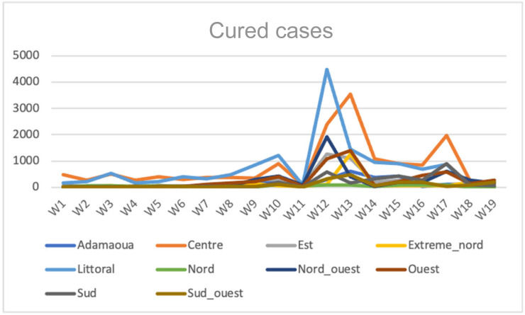
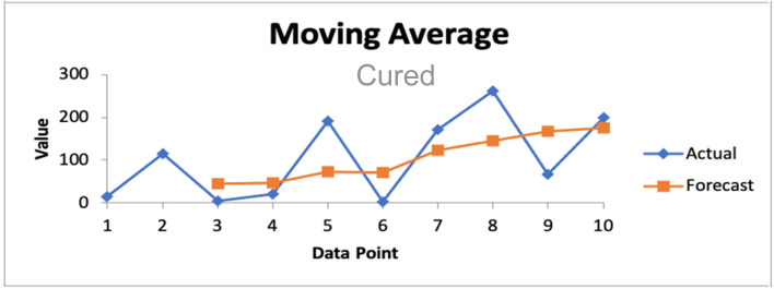
We observed in Fig. 8, Fig. 9, Fig. 10, Fig. 11, Fig. 12 that for cured cases, there is high correlations between Ouest and Center with score 0.9308 and also between Littoral and Nord-Ouest with score 0.936967. The least correlation is between Extreme-Nord and Sud with score 0.04.

Fig. 8.

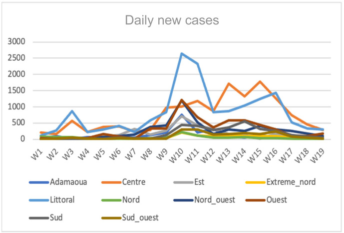
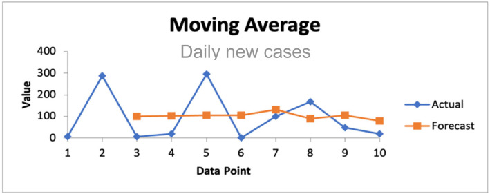
Evolution of the daily new cases numbers in the 10 regions of Cameroon along the second wave between weeks 1 and 10 of 2021.

Fig. 9.

Evolution of the daily new cases numbers in Cameroon along the second wave between weeks 1 and 10 of 2021.

Fig. 10.

Correlations of the cured cases numbers between the 10 regions of Cameroon.

Fig. 11.

Evolution of the cured cases numbers in the 10 regions of Cameroon along the second wave between weeks 1 and 10 of 2021.

Fig. 12.

Evolution of cured cases numbers in Cameroon along second wave between weeks 1 and 10 of 2021.

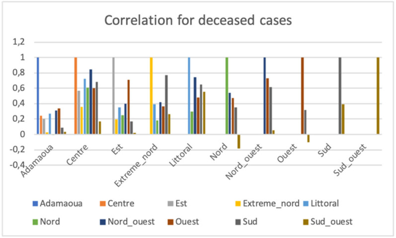
We observed in Fig. 13 three anticorrelations: (i) between Nord and Adamaoua with score −0.00967, (ii) between Nord and Sud-Ouest with score −0.18, and (iii) between Sud-Ouest and Ouest with score −0.09988. The highest correlation is Nord-Ouest and Center with score 0.845.

Fig. 13.

Correlations of the deceased cases numbers between the 10 regions of Cameroon.

5. Application to the COVID-19 outbreak in the world

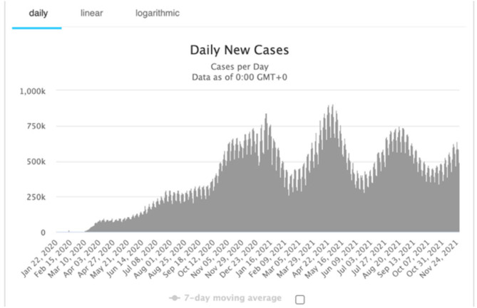
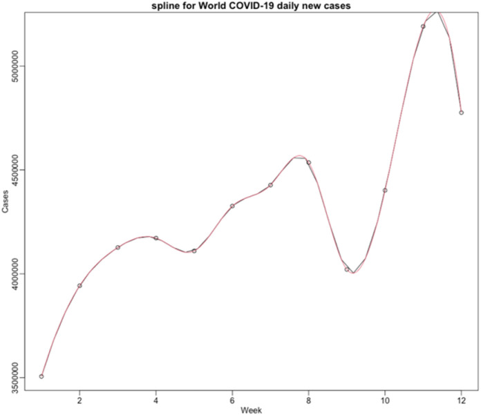
We present in Fig. 14 the global daily new cases of COVID-19 in the world and then smooth the weekly data from October 26 2020 to January 17 2021. The red curve in Fig. 15 represents the cubic spline approximation of the raw data with the following statistics for the second wave: $p$-value $=$ 0.05592, Multiple R-squared MR $=$ 0.9949, Relative Mean Square Error RMSE $=$ 41426.05.

Fig. 14.

World COVID-19 new cases.

From [25].

Fig. 15.

Spline graph for world COVID-19 daily new cases during the second wave.

We calculate the time $t_i$ of the first inflection point $P_I$ of the second wave (which presents a shoulder and no maximum) of the new infectious cases X(t) for the entire world: this time corresponds to a second wave shoulder, in which the maximum of the new cases is not existing for this wave, hence cannot be used for identifying the epidemiologic parameters as in [10], [18], [22]. For that, we have smoothed the raw data of the weekly reported new infectious cases in Fig. 13 by using a cubic spline and we have found $t_i=4$ (weeks).

Then, from Eqs. (10), (11), we get:

$$a=log(S_o-1)/\beta \text{ and }1-6e^{\beta \left(t_i-a\right)}+2e^{2\beta \left(t_i-a\right)}=0$$

with $S_o=7,000,000,000$ and $t_i=4$. Then $a=10$/$\beta$ and $1-6e^{4\beta -10}+2e^{8\beta -20}=0$, from which we get:

$$\beta =2.575\text{ and }a=3.883,$$

which is consistent with the values of the effective reproduction number calculated in [26].

6. Discussion

We have introduced in the paper two new methods, the first for estimating the maximum number of daily reproduction numbers and the second for calculating the rate of transmission by identifying the inflection points of the curve of new infectious cases observed in the framework of the classical Bernoulli model. Then, we have applied these methods to the COVID-19 outbreak in Cameroon, and eventually to the whole world data.

The analysis of the results shows that the model is very sensitive to the length of the contagiousness period r, taken equal to 4$\sigma$, in the case of a Gaussian distribution $\mathcal{N}(m,\sigma )$ for the daily reproduction number. When the value of the standard deviation $\sigma$ increases, the larger its value, the smaller the value of the maximum R${}_{\max }$ of the daily reproduction numbers and vice-versa. In the case of a bimodal distribution, if R${}_{\mathrm{max1}}$ $\ge 0.5$, ${\mathrm{R}}_{\mathrm{max2}}$ will be negative and if we assume that the values of R${}_{\mathrm{max1}}$or ${\mathrm{R}}_{\mathrm{max2}}$ and values of transmission rate for the countries in consideration are close, then the values of R${}_{\mathrm{max1}}$or ${\mathrm{R}}_{\mathrm{max2}}$ are close for all the countries.

The results shown in Table 1, Table 2 are similar to the effective values of ${\mathrm{R}}_{\mathrm{e}}$ given in [23] and to the values of the deterministic R${}_{\mathrm{o}}$ calculated in [8] during the contagiousness period in consideration. This last remark shows the consistency of the results given in the present paper with those obtained from the classical methods of estimation of the effective and deterministic reproduction numbers.

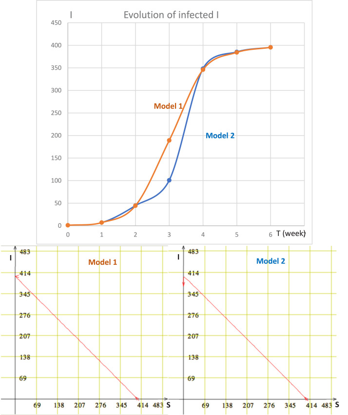
The results obtained by neglecting the mortality due to the COVID-19 outbreak and to the demography of the susceptible population are given on Fig. 16.

Fig. 16.

Top: simulation of the evolution of the number of new infected I in Model 1 (Eq. (9) with $d=\nu =0$) and Model 2 (Eq. (9) with $d=\nu =0.01$). Bottom: simulation of Models 1 and 2 with same initial conditions for infected ($I\left(0\right)=1$) and susceptible individuals ($S\left(0\right)=400$).

The Fig. 16 shows slight differences at the beginning of the epidemic wave between Model 1, corresponding to Eq. (9) in which we have neglected the fertility and the mortality $(d=\nu =0)$ and Model 2, corresponding to Eq. (9) in which we have fixed the demographic balance of susceptibles d to 0.01 and the specific mortality due to the COVID-19 outbreak $\nu$ to 0.01, which are realistic values for Cameroon.

7. Perspectives and conclusion

In this article, we have given a new method for calculating the inflection point of the curve during the exponential phase of a wave. We have then deduced the value of the reproduction number at this inflection point. After that, we have calculated for each region of Cameroon the value of three sets of parameters, one devoted to socio-economic state, another to demography and the last to epidemiology, among which the value of the reproduction number at inflection. We have systematically correlated these sets of parameters and have discussed the relationships between them: the main conclusion is that socio-economic factors are (i) highly positively correlated with each other, (ii) not correlated with epidemiologic parameters (except those corresponding to vaccination and death negatively correlated with the signs of wealth) and (iii) negatively correlated with demographic parameters (namely infant mortality, mean age, fertility and poverty indicators).

In [7], [12], [13], [20], we have already shown different complementary methods, which are available for Cameroon. In a further study, we will use the ARIMA model to analyze COVID-19 incidence pattern for all the waves in Cameroon [7], by taking into account the unidentified infectious cases [13]. We will also identify the main geoclimatic and socio-economic factors explaining the disparities between the different regions of Cameroon.

CRediT authorship contribution statement

J. Waku: Conceptualization, Methodology, Validation, Investigation, Data curation, Visualization, Supervision, Project administration. K. Oshinubi: Conceptualization, Methodology, Software, Validation, Formal analysis, Data curation, Writing – original draft, Writing – review & editing, Visualization. J. Demongeot: Conceptualization, Methodology, Validation, Investigation, Resources, Writing – original draft, Writing – review & editing, Supervision, Project administration.

Declaration of Competing Interest

The authors declare that they have no known competing financial interests or personal relationships that could have appeared to influence the work reported in this paper.

Appendix A. Supplementary data

The data and code used for the analysis can be found in the link below: https://github.com/Honkay/Point-of-Inflexion-and-maximal-reproduction-estimation.git.

References

- 1.Bernoulli D. Essai d’une nouvelle analyse de la mortalité causée par la petite vérole, et des avantages de l’inoculation pour la prévenir, Mem. Acad. Roya. Sci. Paris. 1760 [Google Scholar]
- 2.2022. Cameroon situation reports. Available online: https://reliefweb.int/report/cameroon/ (Accessed 10 February 2022) [Google Scholar]
- 3.Demongeot J., Gaudart J., Lontos A., Promayon E., Mintsa J., Rachdi M. Least diffusion zones in morphogenesis and epidemiology. Int. J. Bifurcation Chaos. 2012;22 [Google Scholar]
- 4.Demongeot J., Gaudart J., Mintsa J., Rachdi M. Demography in epidemics modelling. Commun. Pure Appl. Anal. 2012;11:61–82. [Google Scholar]
- 5.Demongeot J., Griette Q., Magal P. Computations of the transmission rates in SI epidemic model applied to COVID-19 data in mainland China. R. Soc. Open Sci. 2020;7 doi: 10.1098/rsos.201878. [DOI] [PMC free article] [PubMed] [Google Scholar]
- 6.Demongeot J., Griette Q., Magal P. Computations of the transmission rates in SI epidemic model applied to COVID-19 data in mainland China. R. Soc. Open Sci. 2020;7 doi: 10.1098/rsos.201878. [DOI] [PMC free article] [PubMed] [Google Scholar]
- 7.Demongeot J., Oshinubi K., Rachdi M., Hobbad L., Alahiane M., Iggui S., Gaudart J., Ouassou I. The application of ARIMA model to analyse Covid-19 incidence pattern in several countries. J. Math. Comput. Sci. 2022;12:10. [Google Scholar]
- 8.Demongeot J., Oshinubi K., Rachdi M., Seligmann H., Thuderoz F., Waku J. Estimation of daily reproduction rates in COVID-19 outbreak. Computation. 2021;9:109. [Google Scholar]
- 9.Ducrot A., Magal P., Nguyen T., Webb G.F. Identifying the number of unreported cases in SIR epidemic models. Math. Med. Biol. 2020;37:243–261. doi: 10.1093/imammb/dqz013. [DOI] [PubMed] [Google Scholar]
- 10.Ducrot A., Magal P., Nguyen T., Webb G.F. Identifying the number of unreported cases in sir epidemic models. Math. Med. Biol. 2020;37:243–261. doi: 10.1093/imammb/dqz013. [DOI] [PubMed] [Google Scholar]
- 11.2021. Globaldatalab. Available online: https://globaldatalab.org/profiles/region/CMRr110/ (Accessed 10 October 2021) [Google Scholar]
- 12.Griette Q., Demongeot J., Magal P. A robust phenomenological approach to investigate COVID-19 data for France. Math. Appl. Sci. Eng. 2021;2:149–160. [Google Scholar]
- 13.Griette Q., Demongeot J., Magal P. What can we learn from COVID-19 data by using epidemic models with unidentified infectious cases? Math. Biosci. Eng. 2022;19:537–594. doi: 10.3934/mbe.2022025. [DOI] [PubMed] [Google Scholar]
- 14.Liu Z., Magal P., Seydi O., Webb G. Predicting the cumulative number of cases for the COVID-19 epidemic in China from early data. Math. Biosci. Eng. 2020;17:3040–3051. doi: 10.3934/mbe.2020172. [DOI] [PubMed] [Google Scholar]
- 15.Liu Z., Magal P., Seydi O., Webb G. Understanding unreported cases in the Covid-19 epidemic outbreak in Wuhan, China, and importance of major public health interventions. Biology. 2020;9:50. doi: 10.3390/biology9030050. [DOI] [PMC free article] [PubMed] [Google Scholar]
- 16.Magal P., Seydi O., Webb G., Wu Y. A model of vaccination for dengue in the Philippines 2016-2018. Front. Appl. Math. Stat. 2021;7 [Google Scholar]
- 17.McKendrick A.G. Applications of mathematics to medical problems. Proc. Edinb. Math. Soc. 1925;44:1–34. [Google Scholar]
- 18.T. Nguyen, Identifiability of a Class of SIR Models and Applications, (Ph.D. thesis), Bordeaux, 2021,.
- 19.Nkague Nkamba L., Manga T.T. Modelling and prediction of the spread of COVID-19 in Cameroon and assessing the governmental measures (march–september 2020) COVID. 2020;1(2021):622–644. [Google Scholar]
- 20.Oshinubi K., Rachdi M., Demongeot J. Analysis of reproduction number of COVID-19 using current health expenditure as gross domestic product percentage (CHE/GDP) across countries. Healthcare. 2021;9:1247. doi: 10.3390/healthcare9101247. [DOI] [PMC free article] [PubMed] [Google Scholar]
- 21.Oshinubi K., Rachdi M., Demongeot J. Modelling of COVID-19 pandemic vis-à-vis some socio-economic factors. Front. Appl. Math. Stat. 2021;7 [Google Scholar]
- 22.Rahman A., Kuddus M.A. Modelling the transmission dynamics of COVID-19 in six high-burden countries. BioMed Res. Int. 2021 doi: 10.1155/2021/5089184. [DOI] [PMC free article] [PubMed] [Google Scholar]
- 23.2021. Renkulab. Available online: https://renkulab.shinyapps.io/COVID-19-Epidemic-Forecasting/_w_f89fdf90/ [Google Scholar]
- 24.Ross R. An application of the theory of probabilities to the study of a priori pathometry. Proc. R. Soc. Series A. 1916;92:204–230. [Google Scholar]
- 25.2021. Worldometers. Available online: https://www.worldometers.info/coronavirus/ (Accessed 14 November 2021) [Google Scholar]
- 26.Yu C.J., Wang Z.X., Xu Y., Hu M.X., Chen K., Qin G. Assessment of basic reproductive number for COVID-19 at global level: A meta-analysis. Medicine. 2021;100 doi: 10.1097/MD.0000000000025837. [DOI] [PMC free article] [PubMed] [Google Scholar]