SEIR model with unreported infected population and dynamic parameters for the spread of COVID-19

Abstract

Coronavirus disease 2019 (COVID-19) is a contagious disease caused by severe acute respiratory syndrome coronavirus 2 (SARS-CoV-2) that can be transmitted through human interaction. In this paper, we present a Piecewise Susceptible–Exposed–Infectious–Unreported–Removed model for infectious diseases and discuss qualitatively and quantitatively. The parameters are explored by mathematical and statistical methods. Numerical simulations of these models are performed on COVID-19 US data and Python is used in the visualization of results. Outbreak factor is generated by piecewise model to explore the future trend of the US pandemic. Several error metrics are given to discuss the accuracy of the models. The main achievement of this paper is to propose the piecewise model and find the relationship between spread of pandemic and mitigation measures to control it by observing the results of numerical simulations. Performance analysis of piecewise model is presented based on COVID-19 data obtained by ‘worldmeter’.

1. Introduction

Since the end of 2019, the COVID-19 pandemic [1], [2], caused by the severe acute respiratory syndrome coronavirus 2 (SARS-CoV-2), is raging around the world [16]. In December 2019, the first cases of COVID-19 were detected in Wuhan, Hubei Province, China. As of March 11, 2021, more than 118 million confirmed cases have been reported in 219 countries and regions, of which more than 2.621 million died and 66.926 million recovered. At present, the number of confirmed cases is still rising rapidly [3].

Hamer, Ross, and others have done a lot of work in the establishment of mathematical models of infectious diseases until 1927 [7], [10]. Kermack and McKendrick studied the SIR compartmental model during the Black Death in London [7], [14], and the SIS model was established in 1932 [15], [19]. Based on the study of these models, the threshold theory in the dynamics of infectious diseases was proposed [17]. The SIR model of Kermack and McKendrick is the most classic and basic model among infectious disease models and has made a foundational contribution to the study of infectious disease dynamics. The SIR model divides the total population into the following three populations: susceptible $S$, which represents the people who are not infected but are likely to be infected by this type of disease; infectious $I$, which represents the people who have been infected as patients and has the capability of transmitting the disease; and removed $R$, which stands for the people who have been removed from the infected, see also [12], [13] and references therein. Nowadays, the SEIR model [8] is widely used to analyze infectious diseases, see also [9], [20] and references therein. In this model, individuals experience a long incubation duration (the “exposed” category), such that the individual is infected but not yet symptomatic. For example, chicken pox and even vector-borne diseases such as dengue hemorrhagic fever have a long incubation duration where the individual cannot yet transmit the pathogen to others.

The SEIR model is as follows;

$$\frac{dS\left(t\right)}{dt}=-\frac{\beta S\left(t\right)I\left(t\right)}{N}$$ (1)

$$\frac{dE\left(t\right)}{dt}=\frac{\beta S\left(t\right)I\left(t\right)}{N}-\sigma E\left(t\right)$$ (2)

$$\frac{dI\left(t\right)}{dt}=\sigma E\left(t\right)-\gamma I\left(t\right)$$ (3)

$$\frac{dR\left(t\right)}{dt}=\gamma I\left(t\right)$$ (4)

The meaning of each parameter and variable is shown below:

$N$: Total population.

$S\left(t\right)$: The number of susceptible individuals at time $t$. They are not infected at this point.

$E\left(t\right)$: The number of asymptomatic individuals exposed to the virus at time $t$. They are in the incubation period and capable of transmitting the disease but have not exhibited any symptoms.

$I\left(t\right)$: The number of symptomatic infected individuals at time $t$. This group has tested positive and corresponds to the Worldmeter data for active cases. [5]

$R\left(t\right)$: The number of individuals who have been removed from the infected at time $t$ due to either death or recovery.

$\beta$: Transmission rate.

$\gamma$: Removed rate.

$\sigma$: Incubation rate.

The SEIR diagram below shows how individuals move through each compartment in the model (see Fig. 1):

Fig. 1.

SEIR model.

The SEIR model can be applied to most infectious diseases, but there are some limitations when applied to the COVID-19 data. Due to the characteristics of COVID-19, exposed individuals also have the capability of transmitting the disease. The traditional SEIR model assumes that the members of the $E$ compartment are infected but not infectious during the incubation period[8]. The SEIR model also ignores the group of unreported cases. Due to the lack of medical resources and variability in the testing policy, there is no guarantee that all infected people are tested and reported during a wide-spread pandemic. This group of people is likely to become hidden transmitters in the population. The SEIR model with constant parameters cannot be used for long-term simulation. This is because the transmission rate $\beta$ and removed rate $\gamma$ must be changed over a long period of time.

In this paper, we propose the piecewise SEIUR model and the use of a type of least-squares method to estimate the parameters, which overcomes the main difficulty in the SEIR model.

2. SEIUR model

We expect to address the two weaknesses of the SEIR model. First, to overcome the second weakness, the SEIUR model divides the infection equation (3) from SEIR model into two new parts: an unreported symptomatic infection equation (13) and a reported symptomatic infection equation (12). Compartment $I$ represents individuals who are infectious and have been tested (and thus reported). The new compartment $U$ represents people who are symptomatic and infectious but have not been tested for various reasons. Let $f$ be the proportion from $E$ to $I$, and $1-f$ be the proportion from $E$ to $U$. To handle the first weakness, the infectious population $I$ in Eqs. (10), (11) is replaced by the sum of exposed population $E$ and unreported infectious cases $U$, because the individuals in groups $U$ and $E$ have the ability to spread the virus to others during the infection. On the contrary, people in group $I$ were required to be quarantined at home or in hospital and could not infect others.

The establishment of the SEIUR model is based on the following assumptions:

• •Keep first three assumptions same as SEIR model
• •Exposed and Unreported infected individuals are capable of transmitting the disease
• •Reported infectious individuals do not have capability of transmitting the disease
• •Unreported infected individuals cannot become the reported infected individuals

The SEIUR model is given by;

$$\frac{dS\left(t\right)}{dt}=-\frac{\beta S\left(t\right)(E\left(t\right)+U\left(t\right))}{N}$$ (5)

$$\frac{dE\left(t\right)}{dt}=\frac{\beta S\left(t\right)(E\left(t\right)+U\left(t\right))}{N}-\sigma E\left(t\right)$$ (6)

$$\frac{dI\left(t\right)}{dt}=\sigma fE\left(t\right)-\gamma I\left(t\right)$$ (7)

$$\frac{dU\left(t\right)}{dt}=\sigma (1-f)E\left(t\right)-\gamma U\left(t\right)$$ (8)

$$\frac{dR\left(t\right)}{dt}=\gamma (I\left(t\right)+U\left(t\right))$$ (9)

Keep $S\left(t\right)$, $E\left(t\right)$, $R\left(t\right)$, $\beta$, $\gamma$, and $\sigma$ same as SEIR Model.

$I\left(t\right)$: The number of reported infected individuals at time $t$ who are symptomatic and have been tested.

$U\left(t\right)$: The number of individuals infected with the virus but have not been tested at time $t$ and thus not reported.

$f$: The proportion of Exposed individuals that become reported infected individuals (Reported fraction) (see Fig. 2).

Fig. 2.

SEIUR model.

The transition diagram is shown as:

No matter how the SEIR model changes, the core parameters are always $\beta$ and $\gamma$. Therefore, the estimation of $\beta$ and $\gamma$ is particularly vital for both SEIR model and SEIUR model.

2.1. Piecewise SEIUR model

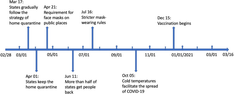
The SEIR and SEIUR models have a fixed value for $\beta$ and $\gamma$ for the entire time period. Since the values of $\beta$ and $\gamma$ are affected by many factors, such as government epidemic prevention measures, quarantine, and vaccination, it is unreasonable to set $\beta$ and $\gamma$ as constants. In addition, another popular method is to use a function to fit $\beta$ and $\gamma$ respectively. This approach makes the values of $\beta$ and $\gamma$ continuous, and the changes are too frequent. Therefore, this paper combines these two ideas, assuming that the values of $\beta$ and $\gamma$ are constant in a period of time, and when entering the next period, the values of $\beta$ and $\gamma$ are updated. The selection of update points is based on the time when the government implemented the relevant strategies or policies, and the phase between two consecutive update points is defined as the “period”. The strategies release timeline is shown in Fig. 3.

Fig. 3.

Strategies [18] release timeline.

Using Fig. 3, we separate the whole time period from 2/28/2020 to 3/16/2021 into eight different parts:

• 1.From 2/28/2020 to 3/16/2020
• 2.From 3/17/2020 to 3/31/2020
• 3.From 4/1/2020 to 4/20/2020
• 4.From 4/21/2020 to 6/10/2020
• 5.From 6/11/2020 to 7/15/2020
• 6.From 7/16/2020 to 10/4/2020
• 7.From 10/5/2020 to 1/15/2021
• 8.From 1/15/2021 to 3/16/2021

For each period $i$, we have an independent SEIUR model, and corresponding specific parameters ${\beta }_i$ and ${\gamma }_i$. The piecewise SEIUR model is shown below:

$$\frac{dS\left(t\right)}{dt}=-\frac{{\beta }_{i}S\left(t\right)(E\left(t\right)+U\left(t\right))}{N}$$ (10)

$$\frac{dE\left(t\right)}{dt}=\frac{{\beta }_{i}S\left(t\right)(E\left(t\right)+U\left(t\right))}{N}-\sigma E\left(t\right)$$ (11)

$$\frac{dI\left(t\right)}{dt}=\sigma fE\left(t\right)-{\gamma }_{i}I\left(t\right)$$ (12)

$$\frac{dU\left(t\right)}{dt}=\sigma (1-f)E\left(t\right)-{\gamma }_{i}U\left(t\right)$$ (13)

$$\frac{dR\left(t\right)}{dt}={\gamma }_i(I\left(t\right)+U\left(t\right))$$ (14)

${\beta }_i$: Transmission rate during the period $i$.

${\gamma }_i$: Removed rate during the period $i$.

Other notations have the same meaning as before and the transition diagram for period $i$ is shown in Fig. 4.

Fig. 4.

SEIUR model for period $i$.

In an epidemic, we can obviously judge whether the epidemic is breaking out or disappearing through the change rate of the number of infected people. In the piecewise SEIUR model, E, I and U represent the number of infections. The difference is that those in E are in the incubation period, while those in I and U have been infected.

Thus, we can conclude that the epidemic is still in outbreak when the change rate of the summation of $E$, $I$ and $U$ is greater than $0$, that is,

$$\frac{d(E+I+U)}{dt}>0$$

which implies

$$\frac{dE}{dt}+\frac{dI}{dt}+\frac{dU}{dt}>0$$

By the SEIUR model

$$\frac{{\beta }_{i}S\left(t\right)(E\left(t\right)+U\left(t\right))}{N}-\sigma E\left(t\right)+\sigma E\left(t\right)-{\gamma }_i(I\left(t\right)+U\left(t\right))>0$$

It follows that $\sigma E\left(t\right)$

$$\frac{{\beta }_{i}S\left(t\right)(E\left(t\right)+U\left(t\right))}{N}-{\gamma }_i(I\left(t\right)+U\left(t\right))>0$$

Since ${\gamma }_i$, $I\left(t\right)$, $U\left(t\right)$ are all positive, we have

$$\frac{{\beta }_i(E\left(t\right)+U\left(t\right))S\left(t\right)}{{\gamma }_i(I\left(t\right)+U\left(t\right))N}>1$$

When the rate of change of $E+I+U<0$, we have that the virus is disappearing.

Using the previous approach, we have that

$$\frac{{\beta }_i(E\left(t\right)+U\left(t\right))S\left(t\right)}{{\gamma }_i(I\left(t\right)+U\left(t\right))N}<1$$

When the rate of change of $E+I+U=0$, we have that the virus is under control and may coexist with humans for a long time.

Therefore, we have

$$\frac{{\beta }_i(E\left(t\right)+U\left(t\right))S\left(t\right)}{{\gamma }_i(I\left(t\right)+U\left(t\right))N}=1$$

By the mathematical analysis above, in each period $i$, the formula of the outbreak factor at time $t$ generated by the piecewise SEIUR model is defined by

$${\left(O\left(t\right)\right)}_i=\frac{{\beta }_i(E\left(t\right)+U\left(t\right))S\left(t\right)}{{\gamma }_i(I\left(t\right)+U\left(t\right))N}$$

And we define $O_i=\overline{O{\left(t\right)}_i}$ to represent the average value of outbreak factor in period $i$.

3. Learning of the piecewise SEIUR model

3.1. Data

The data used in this paper is from the reference website ‘Worldmeter’ [5]. This website provides a variety of real-time statistical data. The website belongs to Dadax, an independent digital media company in the United States. This website records all pandemic data in the United States from February 15, 2020 to the present, and the data is updated daily.

The data is comprised of three different contents. The first is active cases starting from 2/15/2020 to 3/16/2021. The second and third contents are in same period and include the total cases and total deaths respectively. The detail of the contents is shown in Table 1:

Table 1.

Data content of total cases, active cases and total deaths.

Data content	Data description	Data period	Data size
Total cases	Total number of infections	2/15/2020 to 3/16/2021	(1, 396)
	(including deaths and recoveries)
Active cases	Current number of infections	2/15/2020 to 3/16/2021	(1, 396)
	(excluding deaths and recoveries)
Total deaths	Total number of deaths	2/15/2020 to 3/16/2021	(1, 396)

We shift the initial data point from 2/15/2020 to 2/28/2020. Although the United States announced the first case of the coronavirus on 1/21/2020, the lack of effective detection methods and insufficient understanding of the coronavirus have led to the low accuracy of the data in the early stage of the pandemic. Thus, we discarded the data from the early period of the pandemic and set 2/28/2020 as the new initial data point.

In addition to the above three sets of data, this paper also needs the total removed cases and total recovered cases. These two sets of data can be obtained by simple calculations between total cases, active cases, and total deaths. The formulas is followed:

$$\text{Total Removed Cases}=\text{Total Cases}-\text{Active Cases}$$

$$\text{Total Recovered Cases}=\text{Total Removed Cases}-\text{Total Deaths}$$

In previous sections, we clearly explained the reasons for constructing the piecewise model and how we segmented the data into distinct periods.

Table 2 shows the details about each time period.

Table 2.

Split data according to strategies [18].

Period #	Time period	Data size	Related policy
Period 1	2/28/2020 to 3/16/2020	(1, 18)	No control measures implemented
Period 2	3/17/2020 to 3/31/2020	(1, 15)	States gradually follow the strategy
			of home quarantine
Period 3	4/1/2020 to 4/20/2020	(1, 20)	States keep the home quarantine
Period 4	4/21/2020 to 6/10/2020	(1, 51)	Requirement for face masks on public places
Period 5	6/11/2020 to 7/15/2020	(1, 35)	More than half of states get people back
			to work
Period 6	7/16/2020 to 10/4/2020	(1, 81)	Stricter mask-wearing rules
Period 7	10/5/2020 to 12/14/2020	(1, 71)	Cold temperatures facilitate the spread
			of COVID-19
Period 8	12/15/2020 to 3/16/2021	(1, 92)	Vaccination begins

According to the piecewise SEIUR model, in each period $i$, there is a corresponding SEIUR model. In addition to showing the accuracy of SEIUR model in each period $i$, this paper also illustrates the performance of this model in the short future term. In other words, we obtain the SEIUR model in period $i$, and use it to estimate the data at the beginning of period $i+1$. For that reason, the training data for SEIUR model in period $i$ is all data from itself, and the test data consists of the first seven days from period $i+1$. For the last period, since the next period data is not available, we divide the period itself into training data and test data with test data being the last seven days.

3.2. Reported rate estimation and algorithms

Our first goal is to estimate an appropriate value of the proportion $f$. Recalling the definition explained in the previous section, $f$ stands for the proportion of $E$ that become $I$. Let $E\left(t\right)$ represent the exposed individuals in time $t$, $\gamma$ represent the removed rate, $\sigma$ is the incubation rate, $n\left(t\right)$ represent the daily COVID-19 tests per thousand people at time $t$, $p\left(t\right)$ stand for the daily positive rate (the share of COVID-19 tests that are positive) at time $t$, and $N$ is the total population. And we assume that all individuals in $E\left(t\right)$ are newly infected and the effect of new exposed cases from $t$ to $t+\frac{1}{\sigma }$ on the results is ignored, then the proportion $f\left(t\right)$ at time $t$ is given by

$$f\left(t\right)=\frac{\sum _{i=t}^{t+\frac{1}{\sigma }}\left(\frac{n\left(i\right)p\left(i\right)N}{1000}\right)}{E\left(t\right)}.$$ (15)

In fact, the reported rate at time $t$ can be approximately equal to the proportion of $E\left(t\right)$ that would be converted into reported cases. Consequently, to estimate $f\left(t\right)$, $E\left(t\right)$ is served as the denominator, and the numerator should be the number of newly reported cases from time $t$ to the time that all $E\left(t\right)$ is converted into reported cases or unreported cases. By the definition, we have that $\frac{n\left(t\right)p\left(t\right)N}{1000}$ represents the daily positive tests at time $t$. $\frac{1}{\sigma }$ stands for the average number of days it takes for a newly infected individual (in $E$) to move to the next compartment ($I$ or $U$). Hence, ${\sum }_{i=t}^{t+\frac{1}{\sigma }}\left(\frac{n\left(i\right)p\left(i\right)N}{1000}\right)$ can be used to estimate the number of newly reported cases from time $t$ to the time that all $E\left(t\right)$ is converted into reported cases or unreported cases. The result is the formula (15).

Since the number of exposed people cannot be directly counted, it is almost impossible to find relevant statistical data on $E$. Here we use the SEIR model to generate historical data of $E\left(t\right)$. $\sigma$ is $\frac{1}{6}$ assumed in previous section. $\gamma$ is obtained by the least square method. $N$ is the total population of United States. For $n\left(t\right)$ and $p\left(t\right)$, we use data from ‘Our World in Data’ [11], which provide the daily COVID-19 tests per thousand people and the daily positive rate. Now, we can generate the proportion $f\left(t\right)$ at any day $t$.

For simplicity, we define $f=\overline{f\left(t\right)}$ as the constant proportion rate for all data and use it in the numerical simulation.

By the formula (15) and the provided data, we estimate $f=\overline{f\left(t\right)}=0.5937$

We can easily obtain the numerical solution of the SEIUR model and piecewise SEIUR model. The algorithms are shown as Algorithms 1 and 2.

Algorithm 1 Determining the numerical solution of SEIUR model

at all time $t\in \{1,2,\dots ,n\}$

Input:

The initial value of variables: $S\left[0\right]$, $E\left[0\right]$, $I\left[0\right]$, $U\left[0\right]$ and $R\left[0\right]$;

The optimal parameters: $\beta$, $\gamma$, $f$ and $\sigma$;

Total population of the United States: $N$;

The number of iterations or days: $n$;

Output

$S\left[t\right]$, $E\left[t\right]$, $I\left[t\right]$, $U\left[t\right]$ and $R\left[t\right]$ at all time $t\in \{1,2,\dots ,n\}$

Procedure

For$i$ in $1$ to $n$

$S\left[i\right]=S[i-1]-\frac{\beta S[i-1]\left(I[i-1]\right)}{N}$

$E\left[i\right]=E[i-1]+\frac{\beta S[i-1]\left(I[i-1]\right)}{N}-\sigma E[i-1]$

$I\left[i\right]=I[i-1]+\sigma fE[i-1]-\gamma I[i-1]$

$U\left[i\right]=U[i-1]+\sigma (1-f)E[i-1]-\gamma U[i-1]$

$R\left[i\right]=R[i-1]+\gamma (I[i-1]+U[i-1])$

Return$S\left[i\right]$, $E\left[i\right]$, $I\left[i\right]$, $U\left[i\right]$ and $R\left[i\right]$

Algorithm 2 Determining the numerical solution of piecewise SEIUR model

at time $t\in \{p_i,p_i+1,\dots ,p_{i+1}-1\}$ for $i=1\dots n$

where $p_i$ is the start point of period $i$ and $p_1=0$

Input:

The initial value of variables: $S\left[0\right]$, $E\left[0\right]$, $I\left[0\right]$, $U\left[0\right]$ and $R\left[0\right]$;

The optimal parameters for each period $i$: ${\beta }_i$, ${\gamma }_i$, $f$ and $\sigma$;

Total population of the United States: $N$;

The number of iterations or days: $n$;

Output

$S\left[t\right]$, $E\left[t\right]$, $I\left[t\right]$ and $R\left[t\right]$ at all time $t\in \{1,2,\dots ,n\}$

Procedure

For$i$ in $1$ to $n$

For$j$ in $p_i$ to $p_{i+1}-1$

$S\left[j\right]=S[j-1]-\frac{{\beta }_{i}S[j-1]\left(I[j-1]\right)}{N}$

$E\left[j\right]=E[j-1]+\frac{{\beta }_{i}S[j-1]\left(I[j-1]\right)}{N}-\sigma E[j-1]$

$I\left[j\right]=I[j-1]+\sigma fE[j-1]-{\gamma }_{j}I[j-1]$

$U\left[j\right]=U[j-1]+\sigma (1-f)E[j-1]-{\gamma }_{j}U[j-1]$

$R\left[j\right]=R[j-1]+{\gamma }_j(I[j-1]+U[j-1])$

Return$S\left[j\right]$, $E\left[j\right]$, $I\left[j\right]$, $U\left[j\right]$ and $R\left[j\right]$

In the SEIUR model, there are four unknown parameters to be estimated: $\beta$, $\sigma$, $f$, and $\gamma$. We have estimated the proportion of $E$ to $I$ as 0.6, that is, $f=0.6$. The incubation rate of the COVID-19 has been estimated between 2 to 11 days ($2.5\text{th}$ to $97.5\text{th}$ percentile) and the mean incubation period as 6.4 days (95% CI: 5.6–7.7) [6]. Thus, we assume $\sigma =\frac{1}{6}$. Least square method is employed to find the optimal parameters of $\beta$ and $\gamma$. The algorithm is shown as Algorithm 3.

Algorithm 3 Parameter Estimation for SEIUR model

Input

Sequence ${\left\{{\beta }_j\right\}}_{j=0}^{99}=\{0,0.01,0.02,\dots ,0.99\}$;

Sequence ${\left\{{\gamma }_j\right\}}_{j=0}^{99}=\{0,0.01,0.02,\dots ,0.99\}$;

Parameters: $f=0.6$, $\sigma =\frac{1}{6}$;

Numerical Solution (Algorithm 1) for $I$ at day $t$, denoted as $I(t,\beta ,\gamma )$;

Real Data [5] for $I$ at day $t$, denoted as $AI\left(t\right)$

The number of iterations or days: $n$;

Output

Optimal Parameters: $\beta$, $\gamma$

Procedure

For$i$ in $0$ to $99$

For$j$ in $0$ to $99$

$m_{ij}=\frac{1}{n}{\Sigma }_{t=0}^n{(AI\left(t\right)-I(t,{\beta }_i,{\gamma }_j))}^2$

Find$\text{min}\{m_{ij},\text{for}i,j\text{in}0\text{to}99\}$ and corresponding indices $a$ and $b$

Return${\beta }_a$ and ${\gamma }_b$

In the piecewise SEIUR model, we also have $\sigma =\frac{1}{6}$ and $f=0.6$. Parameter estimation of ${\beta }_i$ and ${\gamma }_i$ for each period $i$ is shown in Algorithm 4.

Algorithm 4 Parameter Estimation for piecewise SEIUR model

Input

The number of periods: $k$;

Sequence ${\left\{{\beta }_j\right\}}_{j=0}^{99}=\{0,0.01,0.02,\dots ,0.99\}$;

Sequence ${\left\{{\gamma }_j\right\}}_{j=0}^{99}=\{0,0.01,0.02,\dots ,0.99\}$;

Parameters: $f=0.6$, $\sigma =\frac{1}{6}$;

Numerical Solution (Algorithm 2) for $I$ at day $t$, denoted as $I(t,\beta ,\gamma )$;

Real Data [5] for $I$ at day $t$, denoted as $AI\left(t\right)$;

The number of iterations or days: $n$;

Note that: $\{0,1,2,\dots ,n\}=U_{i=1}^k\{p_i,p_i+1,\dots ,p_{i+1}-1\}$;

where $p_i$ is the start point of period $i$ and $p_1=0$;

Output

Optimal Parameters: $({\beta }_i$, ${\gamma }_i)$ for all $i$ in $0$ to $k$

Procedure

For$i$ in $1$ to $k$

For$j$ in $0$ to $99$

For$g$ in $0$ to $99$

$m_{ijg}=\frac{1}{p_{i+1}-pi}{\Sigma }_{t=p_i}^{p_{i+1}}{(AI\left(t\right)-I(t,{\beta }_j,{\gamma }_g))}^2$ (Mean Square Error)

Find$\text{min}\{m_{ijg},\text{for}j,g\text{in}0\text{to}99\}$ and corresponding indices $a_i$ and $b_i$

Return${\beta }_{a_i}$ and ${\gamma }_{b_i}$

4. Simulation results

4.1. Parameter estimation results

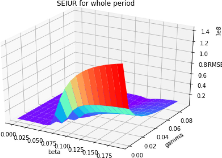
Based on the parameter estimation Algorithm 3, we estimate the parameters $\beta$ and $\gamma$ for SEIUR model in this section. Fig. 5 is the 3D error graph for different values of $\beta$ and $\gamma$.

Fig. 5.

3D error graph with different $\beta$ and $\gamma$ for SEIUR model.

We know that the optimal parameters can be derived from the lowest error point. For the SEIUR model, the optimal parameters are $\beta =0.13$ and $\gamma =0.08$

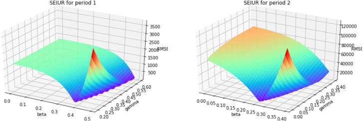
Based on the parameter estimation Algorithm 4, we estimate the parameters ${\beta }_i$ and ${\gamma }_i$ for piecewise SEIUR model in each period $i$. Fig. A.18, Fig. A.19, Fig. A.20, Fig. A.21 are the 3D error graphs showing the optimal values of parameters for each period.

Fig. A.18.

3D error graph for different $\beta$ and $\gamma$ for periods 1 and 2.

Fig. A.19.

3D error graph for different $\beta$ and $\gamma$ for periods 3 and 4.

Fig. A.20.

3D error graph for different $\beta$ and $\gamma$ for periods 5 and 6.

Fig. A.21.

3D error graph for different $\beta$ and $\gamma$ for periods 7 and 8.

Applying the same method from the SEIUR model to the piecewise SEIUR model, we can find the $\beta$ and $\gamma$ related to the lowest error for each period $i$. This allows us to generate the optimal parameters for all periods in Table 3.

Table 3.

Optimal model parameters by period.

Period	$\beta$	$\gamma$
1	0.44	0.36
2	0.26	0.10
3	0.10	0.04
4	0.03	0.01
5	0.08	0.03
6	0.06	0.03
7	0.11	0.06
8	0.10	0.05

4.2. Performance

Fig. 6 shows the numerical simulation results of the SEIUR model on all data. We find that when simulating all of the data at once, the SEIUR model can successfully simulate the trend of data, but it cannot accurately reflect the true value of the data at each point. We have a more intuitive reflection in the error analysis in the next section.

Fig. 6.

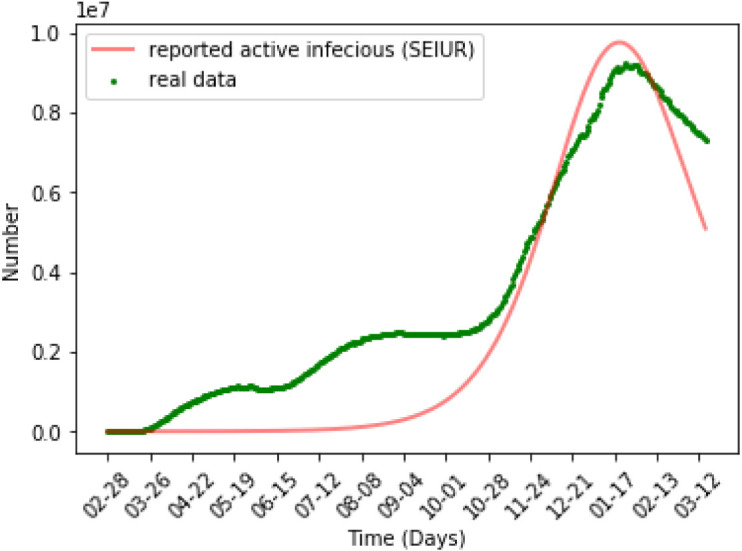
Numerical simulation for SEIUR.

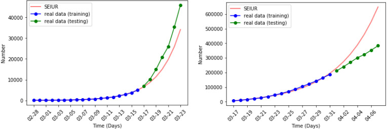
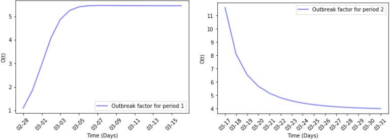
Fig. 7 shows the estimated reported active cases and the real data in periods 1 and 2 where the blue dots are training data and the green dots are test data. Fig. 8 shows the daily outbreak factor in periods 1 and 2. In period 1, no control measures were implemented which led to an exponential outbreak, and we calculate that $O_1=4.9461$ in period 1. This is much greater than 1. This is consistent with what we proved in previous section: when $O\left(t\right)$ is much greater than 1, the pandemic is in a major outbreak stage. Observing the simulation results on the test data, the SEIUR model in the first period can still simulate the data at the beginning of the second period very well. This also means that at the beginning of the second period the home quarantine strategy has not yet contributed to a significant impact, and the pandemic was still breaking out. The $O\left(t\right)$ of the entire second period also confirmed this point. In this period, $O_2=4.8743$, which is slightly lower than that of the period 1 but still far greater than 1. This indicates that in the middle and late stages of period 2, the home quarantine strategy has achieved initial results, but the epidemic was still in outbreak. The test data of period 2 showed that at the beginning of the period 3, the true value of the test data is significantly smaller than the results obtained by SEIUR model generated from parameters estimated in period 2. This implies that the home quarantine strategy implemented in the period 2 achieved a significant effect in the period 3.

Fig. 7.

Numerical simulation in periods 1 and 2. (For interpretation of the references to color in this figure legend, the reader is referred to the web version of this article.)

Fig. 8.

Outbreak factor in periods 1 and 2.

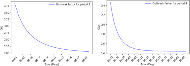
Fig. 9, Fig. 10 show the results of the numerical simulations and the outbreak factor in periods 3 and 4. $O_3=2.3412$ in period 3, which has a 52% decrease compared to period 2. This confirms the analysis made in the discussion of period 2. The home quarantine strategy has slowed the spread of the epidemic. In period 4, mask wearing further reduced the spread of pandemic. The figure about period 4 illustrates the growth rate of the active cases has decreased compared to period 3 and reached the first turning point at the end of May. Quantitatively, $O_4=1.5362$ in period 4, which is a decrease of 34% compared to period 3.

Fig. 9.

Numerical simulation in periods 3 and 4.

Fig. 10.

Outbreak factor in periods 3 and 4.

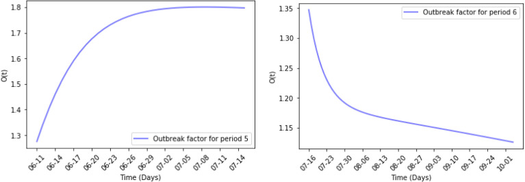
Fig. 11, Fig. 12 show the results of numerical simulations and outbreak factors in periods 5 and 6. In period 5, many states are relaxing their restrictions, with more than half set to be partially reopened. This led to the pandemic rebounding rapidly after reaching the first turning point and active cases starting to rise again. The average outbreak factor also rose from 1.5362 to 1.7176. In period 6, stricter mask-wearing rules slowed the spread of pandemic, and the second turning point was reach at the end of August with $O_6=1.1660$.

Fig. 11.

Numerical simulation in periods 5 and 6.

Fig. 12.

Outbreak factor in periods 5 and 6.

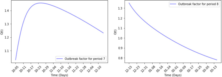
Fig. 13, Fig. 14 show the results of numerical simulations and outbreak factors in periods 7 and 8. Winter brings shorter days and lower temperatures to the United Stated which facilitate the spread of COVID-19. Period 7 shows this process. With the advent of winter, active cases began to increase again after reaching the second turning point, and $O_7$ rose back to 1.3414. Period 8 is the latest period so far, and vaccinations began on the first day of this period. The graph in period 8 shows that the vaccination quickly controlled the spread of the pandemic, and the third turning point appeared at the end of January 2021. So far, the reported active cases have continued to decline. In period 8, $O_8=0.9991$ which is less than 1. If this continues, the epidemic is likely to be completely controlled in the next few months.

Fig. 13.

Numerical simulation in periods 7 and 8.

Fig. 14.

Outbreak factor in periods 7 and 8.

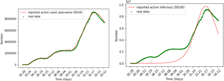
Fig. 15 shows the numerical simulation results of the piecewise SEIUR model and SEIUR model, where the result of piecewise SEIUR is obtained by combining the graphs of eight periods. It can be seen from the figure that the piecewise SEIUR model performs better than the SEIUR model. This also means that it is reasonable to divide a long periods of time into different sub-period according to policy dates, and then use the SEIUR model to simulate each period respectively.

Fig. 15.

Numerical simulation for piecewise SEIUR and SEIUR.

4.3. Error metrics

After performing the numerical simulation of the model, error analysis is an effective way to assess the accuracy of the model. There are many error metrics, such as mean absolute error (MAE), mean absolute percentage error (MAPE), symmetric mean absolute percentage error (SMAPE), mean squared error (MSE), root mean squared error (RMSE) and $R^2$ score. In this section we discuss several representative error metrics for error analysis.

The Mean Absolute Percentage Error (MAPE) [4] is one of the most commonly used to measure model accuracy. It is the average of the relative error. It is given by the following formula:

$$\text{MAPE}=\frac{1}{n}\cdot \sum _{i=1}^n\left|\frac{rea{l}_i-estimat{e}_i}{rea{l}_i}\right|\times 100\text{\%}$$

The Mean Absolute Error (MAE) [4] is a popular error metric to measure model accuracy. As the name implies, it is the average of the absolute error. The formula is shown below:

$$\text{MAE}=\frac{1}{n}\cdot \sum _{i=1}^n|rea{l}_i-estimat{e}_i|$$

The Mean Squared Error (MSE) [4] is an error metric to measure model accuracy. Since MSE is a continuous function, it is often used together with the least square method and gradient descent method. It is defined as the average squared error. The formula is shown below:

$$\text{MSE}=\frac{1}{n}\cdot \sum _{i=1}^n{\left(rea{l}_i-estimat{e}_i\right)}^2$$

The $R^2$ score [4] function computes the coefficient of determination, usually denoted as $R^2$. It represents the proportion of variance (of $y$) that has been explained by the independent variables in the model. It provides an indication of goodness of fit and therefore a measure of how well unseen samples are likely to be predicted by the model through the proportion of explained variance.

If ${\hat{y}}_i$ is the predicted value of the $i$th sample and $y_i$ is the corresponding true value for total $n$ samples, the estimated $R^2$ is defined as:

$$R^2(y,\hat{y})=1-\frac{\sum _{i=1}^n{(y_i-{\hat{y}}_i)}^2}{\sum _{i=1}^n{(y_i-\overline{y})}^2}$$

$${\text{MAPE}}_{\text{PW-SEIUR}}=4.083\text{\%}$$

$${\text{MAPE}}_{\text{SEIUR}}=59.526\text{\%}$$

From the results shown in Fig. 16, it can be seen that the piecewise SEIUR model has a small MAPE in each period and over the entire data. Specifically, the MAPE from period 3 to period 8 is lower than 5%, the MAPE in all periods is lower than 10%, and the MAPE in the entire period is only 4%. In contrast, the MAPE of SIEIUR model exceeds 50%.

$${\text{MAE}}_{\text{PW-SEIUR}}=1.12\times 10^5,{\text{MSE}}_{\text{PW-SEIUR}}=2.50\times 10^{10}$$

$${\text{MAE}}_{\text{SEIUR}}=1.041\times 10^6,{\text{MSE}}_{\text{SEIUR}}=1.55\times 10^{12}$$

Fig. 16.

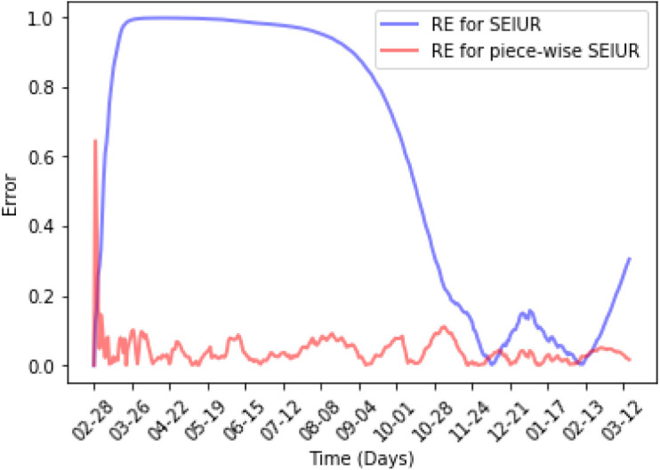
Relative error for Piecewise SEIUR and SEIUR.

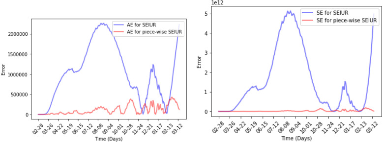
MAE and MSE are shown in Fig. 17 and produce the same results. No matter which error metric is used, the piecewise SEIUR model has a better performance than the SEIUR model. Quantitatively, the error of piecewise SEIUR model under the MAE metric is only one-tenth of that of the SEIUR, and under the MSE metric it is only one-sixth.

$${\text{R}}_{\text{PW-SEIUR}}^2=0.9972$$

$${\text{R}}_{\text{SEIUR}}^2=0.8239$$

Fig. 17.

Absolute error (AE) and Square error (SE) for Piecewise SEIUR and SEIUR.

The results from $R^2$ score also illustrate that piecewise SEIUR model has an almost perfect fitting. The $R^2$ score of piecewise SEIUR model is approximately equal to 1 (see Table 4).

Table 4.

Error table for SEIUR and Piecewise SEIUR models.

	Error metrics
Models name	MAPE	$R^2$	MAE	MSE
Piecewise SEIUR model	4.083%	0.9972	$1.12\times 10^5$	$2.50\times 10^{10}$
SEIUR model	59.526%	0.8239	$1.041\times 10^6$	$1.55\times 10^{12}$

5. Conclusion

In this paper, we have presented the SEIUR model and the piecewise SEIUR model. These two models are tested on COVID-19 data in the United States to demonstrate their performance. We estimated piecewise parameters $\beta$ and $\gamma$ for each period of the model. These two models were applied to COVID-19 data in the United States to demonstrate their performance. The piecewise SEIUR model is seen to produce higher simulation accuracy than the SEIUR model. The MAPE of the piecewise SEIUR is only 4%. The error of piecewise SEIUR model under MAE and MSE metrics is far less than that of the SEIUR model. The $R^2$ score of the piecewise SEIUR model is 0.9972 which is close to 1. The outbreak factor generated by the piecewise SEIUR model can be applied to highlight the impact of the epidemic prevention strategies in each period. This also provides a mathematical tool for future research on the impact of different strategies on epidemics.

Appendix. Error graphs for the seiur model

See Fig. A.18, Fig. A.19, Fig. A.20, Fig. A.21.