Deep Learning-based Classification of Preclinical Breast Cancer Tumor Models Using Chemical Exchange Saturation Transfer MRI

Abstract

Chemical Exchange Saturation Transfer (CEST) MRI has shown promise for classifying tumors based on their aggressiveness, but CEST contrast is complicated by multiple signal sources and thus prolonged acquisition times are often required to extract the signal of interest. We investigated whether deep learning could help identify pertinent Z-spectral features for distinguishing tumor aggressiveness as well as the possibility of acquiring only the pertinent spectral regions for more efficient CEST acquisition. Human breast cancer cells, MDA-MB-231 and MCF-7, were used to establish bi-lateral tumor xenografts in mice to represent higher and lower aggressive tumors, respectively. A convolutional neural network (CNN)-based classification model, trained on simulated data, utilized Z-spectral features as input to predict labels of different tissue types, including MDA-MB-231, MCF-7, and muscle tissue. Saliency maps reported the influence of Z-spectral regions on classifying tissue types. The model was robust to noise with an accuracy of over 91.5% for low and moderate noise levels in simulated testing data (SD of noise less than 2.0%). For in vivo CEST data acquired with a saturation pulse amplitude of 2.0 μT, the model had a superior ability to delineate tissue types compared to Lorentzian difference (LD) and MTR_asym analysis, classifying tissues to the correct types with a mean accuracy of 85.7%, sensitivity of 81.1%, and specificity of 94.0%. The model performance did not improve substantially when using data acquired at multiple saturation pulse amplitudes or when adding LD or MTR_asym spectral features, and did not change when using saliency map-based partial or downsampled Z-spectra. This study demonstrates the potential of CNN-based classification to distinguish between different tumor types and muscle tissue, and speed up CEST acquisition protocols.

1. INTRODUCTION

Chemical Exchange Saturation Transfer (CEST) MRI is an emerging imaging approach that has shown promise for detecting molecular level changes in various cancers^1–9. CEST MRI detects the interaction between exchangeable protons in low concentration solute molecules and bulk water by selectively labelling solute protons using radiofrequency (RF) irradiation. Variations in the relative concentration or the chemical microenvironment of these solute protons change their contributions to the CEST contrast. Several previous breast tumor studies applying CEST MRI to cells, animals, and humans have demonstrated the potential of CEST for metabolite detection, tumor characterization, and treatment assessment^5,10–13.

CEST MRI studies often try to quantify a signal at a specific saturation frequency but most often a series of images at multiple saturation frequencies (Z-spectral images) is acquired to assist in separating the desired contrast from other signal sources¹⁴. Interfering signals include direct water saturation (DS)¹⁵, other types of exchangeable protons¹⁶, semi‐solid magnetization transfer contrast (MTC)¹⁷, and relayed Nuclear Overhauser Effects (rNOEs) of mobile macromolecules^1,18–21. CEST acquisition of a full Z-spectrum may result in excessive scan times and may still result in erroneous or unreliable CEST maps.

Machine learning is being adopted rapidly in the medical imaging community for tasks such as segmentation, parameter estimation, and tumor classification^22–24. In CEST MRI, machine learning has previously been successfully applied to classify Z-spectra of pancreatic cancer²⁵. Since then, deep learning^26,27 has been proposed to learn data features more effectively and perform complex tasks. The neural network in CEST MRI involved learned features of 3T CEST signals to map with 9.4T ultrahigh-field CEST contrast²⁸. Uncertainty quantification using the DeepCEST neural network provided a robust estimation of Lorentzian parameters for both healthy and human brain tumor tissue at 3T and demonstrated the reliability of the neural network²⁹. In addition, artificial neural network (ANN) CEST was used to map the concentration of phosphocreatine (PCr) in human skeletal muscle as well as its guanidinium proton exchange rates, B₀ and B₁ field inhomogeneities simultaneously³⁰.

Here, we introduce a deep learning-based classification approach to distinguish different types of breast tumors with CEST MRI in a preclinical model. A bi-lateral human tumor xenograft model of MDA-MB-231 and MCF-7 cancer cells (known to be higher and lower aggressive, respectively) was used to assess the feasibility of using Z-spectra to classify these tissue types and separate them from normal muscle tissue. The convolutional neural network (CNN) also provided a saliency map that reported the impact of saturation frequencies on predicting class labels. After training, robustness to noise was tested on simulated Z-spectra and the classification approach was then tested on the bi-lateral human tumor xenograft models.

2. MATERIALS AND METHODS

2.1. Cells and animal model

All animal experiments were performed in accordance with the Animal Care and Use Committee guidelines of the Johns Hopkins University, USA. MCF-7 (lower aggressive human breast cancer cells) and MDA-MB-231 (higher aggressive human breast cancer cells) were obtained from American Type Culture Collection (ATCC). Cells were cultured in Dulbecco’s Modified Eagle Medium (DMEM) supplemented with 10% PBS, 100 μg/ml penicillin, 100 U/ml streptomycin, at 37 °C in a humidified atmosphere containing 5% CO₂. Xenograft tumors were induced in 6 – 8-week-old severe combined immune deficiency (SCID-ICR) female mice by injecting MDA-MB-231 and MCF-7 cancer cells (10⁶ cells /100 μl) into the right and left flank of mice (n=5), respectively.

2.2. MR imaging

MR imaging was performed 3–5 weeks post-implantation with the mice anesthetized using 0.5–2% isoflurane prior to imaging. MRI images were acquired on a Bruker 11.7T horizontal MRI scanner, with a 72-mm quadrature volume resonator for transmission and an 8-channel phased array RF coil for reception. CEST MRI images at 81 frequency offsets between ±6 ppm with step size of 0.15 ppm were acquired using a continuous-wave (CW) saturation pulse, followed by a single-slice rapid acquisition with relaxation enhancement (RARE) sequence (RARE factor = 23). S₀ image was collected at 40 ppm. The scanning time for each saturation power was 14 mins. The other imaging parameters were as follows: t_sat = 4,000 ms, TR/TE = 10,000 ms/ 3.49 ms, saturation pulse amplitudes (B_1,sat) = 0.5, 1.0, and 2.0 μT. The slice thickness was 1 mm, field of view (FOV) was 28 × 21 mm², and matrix size was 64 × 64.

2.3. Image processing

The CEST images were normalized by the S₀ image. B₀ inhomogeneity in CEST images was corrected on a voxel-by-voxel basis by finding the frequency offset of direct water saturation chemical shift in Z-spectra at B_1,sat = 0.5 μT³¹. Median filter with kernel size of 3 was applied on CEST images to improve signal-to-noise (SNR).

For analysis, three regions of interests (ROIs) were drawn manually within MDA-MB-231, MCF-7, and muscle tissue. The multi-B_1,sat Z-spectra of Mouse #1 were fitted with a seven-pool Bloch-McConnell equation³² to obtain parameters, including water (0 ppm), guanidinium protons at 2.1 and 2.6 ppm, Amide protons at 3.5 ppm, rNOEs at −3.5 ppm, symmetric (0 ppm) and asymmetric (−2.3 ppm) MTC pools. R² (goodness of fit), as defined by³³:

$${\text{R}}^2=1-\frac{{\sum }_{\text{i}}{\left({\text{S}}_{\text{exp},\text{ i}}-{\text{S}}_{\text{fit},\text{i}}\right)}^2}{{\sum }_{\text{i}}{\left({\text{S}}_{\text{exp},\text{ i}}-\overline{{\text{S}}_{\text{exp}}}\right)}^2}$$ [1]

was used to evaluate discrepancies between the fitted (S_fit) and experimental data (S_exp), and where i is the index of the saturation frequency and $\overline{{\text{S}}_{\text{exp}}}$ is the average value of all the data points in the Z-spectrum.

For comparison, CEST contrast was also quantified using magnetization transfer ratio asymmetry (MTR_asym)^34–36, which takes the difference in normalized signal intensity between opposite frequencies (±Δω) about the water resonance in the water saturation spectrum (Z-spectrum), defined by:

$${\text{MTR}}_{\text{asym}}\left(\Delta \omega \right)=\frac{{\text{S}}_{\text{sat}}\left(-\Delta \omega \right)-{\text{S}}_{\text{sat}}\left(+\Delta \omega \right)}{{\text{S}}_0}$$ [2]

where S_sat(-Δω) and S_sat(+Δω) are the water signal intensities after saturation with RF irradiation at negative and positive frequency offset (Δω) relative to water, and S₀ is an image acquired without RF saturation.

In addition, Lorentzian difference (LD) analysis, which employs a single Lorentzian line to represent DS and then takes the difference from experimental data to quantify saturation transfer contrast^37–40, was used to quantify CEST contrast. Lorentzian fitting of the water signal was performed by using the Z-spectral ranges −0.5 to 0.5 ppm and 5.5 to 6.0 ppm¹⁸. The spectra of residual CEST signals were obtained by subtracting the experimental Z-spectra from the fitted spectra.

All Bloch equation-based fitting and simulations were performed on MATLAB 2019a using source code downloaded from http://www.cest-sources.org⁴¹. Other data processing was performed using custom-written scripts in Python. Statistical analyses were performed with Prism8 (GraphPad Software). Groups were considered to be different when a Wilcoxon Rank‐Sum analysis showed with P ≤ 0.05 between groups.

2.4. Classification model

2.4.1. Training data for classification

Bloch equation fitting parameters were further used to generate simulated Z-spectra for MDA-MB-231, MCF-7, and muscle tissue. The Z-spectra contained 81 frequency offsets between ±6 ppm with t_sat = 4,000 ms, and B_1,sat = 0.5, 1.0, 2.0 μT for the CW saturation pulse. The B₀ field was set to 11.7 T. To mimic true signal variation, concentration ranges were set for guanidinium, amide, rNOE, and MTC pools, accompanied by different levels of Rician noise⁴² with a mean of 0 and standard deviation (SD) of 0.3%, 0.5%, and 0.8% were added to the simulation data. Finally, a total of 300,000 simulated Z-spectra (100,000 for each class) were obtained and used to train the classification model.

2.4.2. Classification architecture and training

The CNN-based classification model (using Z-spectra acquired with B_1,sat = 2.0 μT), which took 1D vectors with 81 elements that represent Z-spectra as inputs, consisted of four convolution and max pooling layers, one fully connected layer, and one classification layer (with softmax function as activation function) to learn Z-spectral features of different tissue types (Figure 1). The dropout regularization with value of 0.2 was added before the fully connected layer. A rectified linear unit (ReLU) was used as an activation function and categorical cross-entropy was used as a loss function. Training data were randomly split for training and validation (80% and 20% of the sample, respectively). The stochastic gradient descent (SGD) optimization algorithm⁴³ with learning rate of 10⁻³ was used to train the model for 200 epochs with a batch size of 64. Early stopping strategy was employed when validation losses did not improve within 5 consecutive epochs. Hyperparameter estimation was performed by grid search frameworks as described in the Supporting Information (Figure S8). Notably, the saliency vectors obtained from the CNN input vectors estimate the influence of Z-spectral features on the output classification⁴⁴. The saliency maps were obtained for randomly selected voxels over the respective regions of mice. The simulated three-class Z-spectra were used for training, and in vivo Z-spectra (except for Mouse #1, which was used for Bloch equation fitting and tuning hyperparameters of CNN) were used as testing data. The CNN model was implemented in the Keras framework⁴⁵ with Tensorflow backend⁴⁶.

Figure 1.

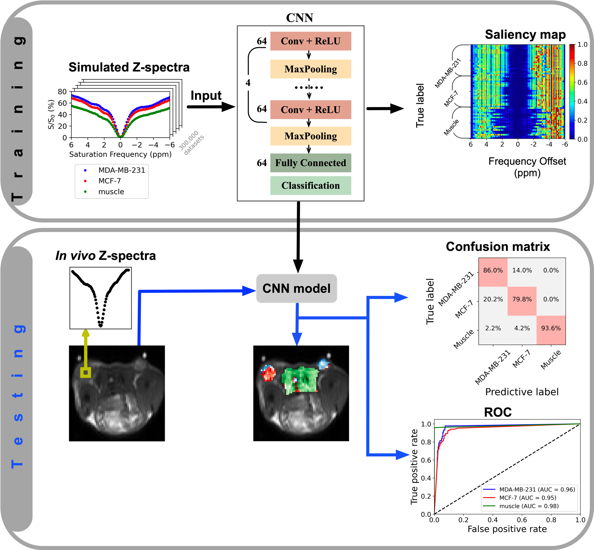
Illustration of the classification model. In the training stage, the simulated Z-spectra of MDA-MB-231, MCF-7, and muscle tissue are used to train the multi-class classification model which distinguishes the three tissue types. CNN model and saliency map (which is computed using keras-vis package⁴⁷) are obtained. In the testing stage, the voxels to be classified are input into the CNN model to predict labels, and then, the confusion matrix and AUC of the receiver operating curve (ROC) are obtained.

The total training time was 4 hours 43 mins and the prediction speed was 220 observations per second on a personal computer (2.6 GHz Intel Core i7 with 16 G memory).

2.5.3. Evaluation of classification performance

ROIs were drawn over known regions of MDA-MB-231, MCF-7, and muscle tissue. The model was measured by a confusion matrix, which shows the true positive (TP) rates versus false negative (FN) rates, and true negative (TN) rates versus false positive (FP) rates. Accuracy, sensitivity, and specificity were calculated from the confusion matrix, as following:

$$\text{Accuracy}=\frac{\text{TP}+\text{TN}}{\text{TP}+\text{TN}+\text{FN}+\text{FP}}\times 100\%$$ [3]

$$\text{Sensitivity}=\frac{\text{TP}}{\text{TP}+\text{FN}}\times 100\%$$ [4]

$$\text{Specificity}=\frac{\text{TN}}{\text{TN}+\text{FP}}\times 100\%$$ [5]

In addition, the performance of the model was evaluated by the area under curve (AUC) of the receiver operating curve (ROC).

3. RESULTS

3.1. Bloch equation fitting and simulation of Z-spectra

The Z-spectra of two tumors and muscle tissue (circles in Figure 2) from Mouse #1 show clear dips centered at 2.0, 3.5, and −3.5 ppm, which we attributed to guanidinium protons (mobile proteins in tumor and creatine (Cr) in muscle), amide protons (mobile proteins), and rNOEs of aliphatic protons in mobile proteins, respectively. Z-spectra from muscle tissue contained an additional peak at 2.6 ppm, known to be from PCr guanidinium protons. These obvious peaks as well as the water and MTC pools were selected as pools in the Bloch equation fitting. The choice of both symmetric and asymmetric MTC pools was based on the assumption of saturation transfer originating directly from solid-like groups around water (e.g., −OH and bound water, symmetric) and relayed from aliphatic protons from lipids (asymmetric). Assuming a single resonance, the fitting results (Figure 2) indicate that that the peaks at 2.0 and 3.5 ppm in muscle have lower exchange rates (see from the narrower lineshape) compared to tumors. The fitting results at B_1,sat = 0.5, 1.0, and 2.0 μT are shown in Figure 2, and the obtained fitting parameters are shown in Table 1. The mean R² of three tissues under multi-B_1,sat was better than 0.98. Based on the fitting parameters, concentration ranges for guanidinium, amide, relayed NOE, and MTC pools were set to generate simulated Z-spectra for use as training dataset (Table 1). Larger concentration ranges were assigned to the pools with higher concentrations.

Figure 2.

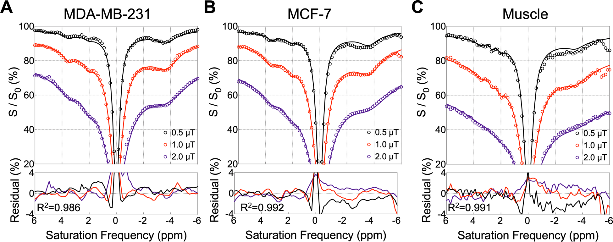
Fitting results for Z-spectra of ROIs taken in (A) MDA-MB-231, (B) MCF-7, and (C) muscle tissue at B_{1, sat} = 0.5, 1.0, 2.0 μT from Mouse #1. The ROIs used for the Z-spectra are shown in Figure 4D. Experimental Z-spectra are shown with circles and fitted Z-spectra with solid lines. The bottom row shows the residuals between experimental and fitted Z-spectra for three B_1,sat values and indicates the mean R² (goodness of fit) over the three B_1,sat values.

Table 1.

Parameters used for fitting Z-spectra and for generating simulation data of MDA-MB-231 / MCF-7 / muscle tissue.

Pool*	Peak position (ppm)	T1 (s)	T2 (ms)	Exchange Rate (Hz)	Concentration (mM)
					Fitting	Simulation range
Water	0.0	1.20	29	1	111,000	111,000
		1.00	19
		1.31	14
Mobile protein, Cr (Guanidinium)	2.1	1	2	600	110	90 – 130
				600	150	130 – 170
				180	160	140 – 180
PCr (Guanidinium)	2.6	1	5	\	\	\
				\	\	\
				160	90	70 – 110
Mobile protein (Amide)	3.5	1	1	100	180	160 – 200
				100	260	240 – 280
				40	200	180 – 220
Mobile protein, aliphatic protons relayed NOE	−3.5	1	0.45	35	900	850 – 950
					1,200	1,150 – 1,250
					650	600 – 700
Symmetric MTC	0.0	1	0.07	20	5,900	4,000 – 6,500
					7,200	7,100 – 8,500
					6,400	4,500 – 9,000
Asymmetric MTC	−2.3	1	0.03	20	200	100 – 500
					1,400	1,200 – 1,800
					7,800	7,500 – 8,500

Abbreviations: Cr, creatine; MTC, magnetization transfer contrast; NOE, nuclear Overhauser effects; PCr, phosphocreatine.

^*Pools were chosen to consist of the dominant protons at that frequency.

3.2. Simulations: Effect of noise on classification accuracy

The influence of noise on the ability of the classification model at B_1,sat = 2.0 μT to distinguish between different tissue types is illustrated using synthetic Z-spectra in Figure 3. The simulated data (3,000 sets) with a larger concentration range than simulated training data and different levels of noise were used as testing data. The model performed well with low noise levels (noise SD < 0.8%) and achieved accuracies greater than 98.7%. The increased noise levels (noise SD between 1.0% and 2.0%) made it difficult to visually distinguish Z-spectra from different tissues. However, the classification model was still able to distinguish between the three tissue types with an accuracy of greater than 91.5% with these moderate noise levels. When adding high levels of noise (noise SD > 2.5%), the Z-spectra of MDA-MB-231 and MCF-7 closely resembled each other and the classification accuracy was greatly reduced (lower than 87.0%). With very high noise levels, noise SD = 4%, the accuracy was 72.4%.

Figure 3.

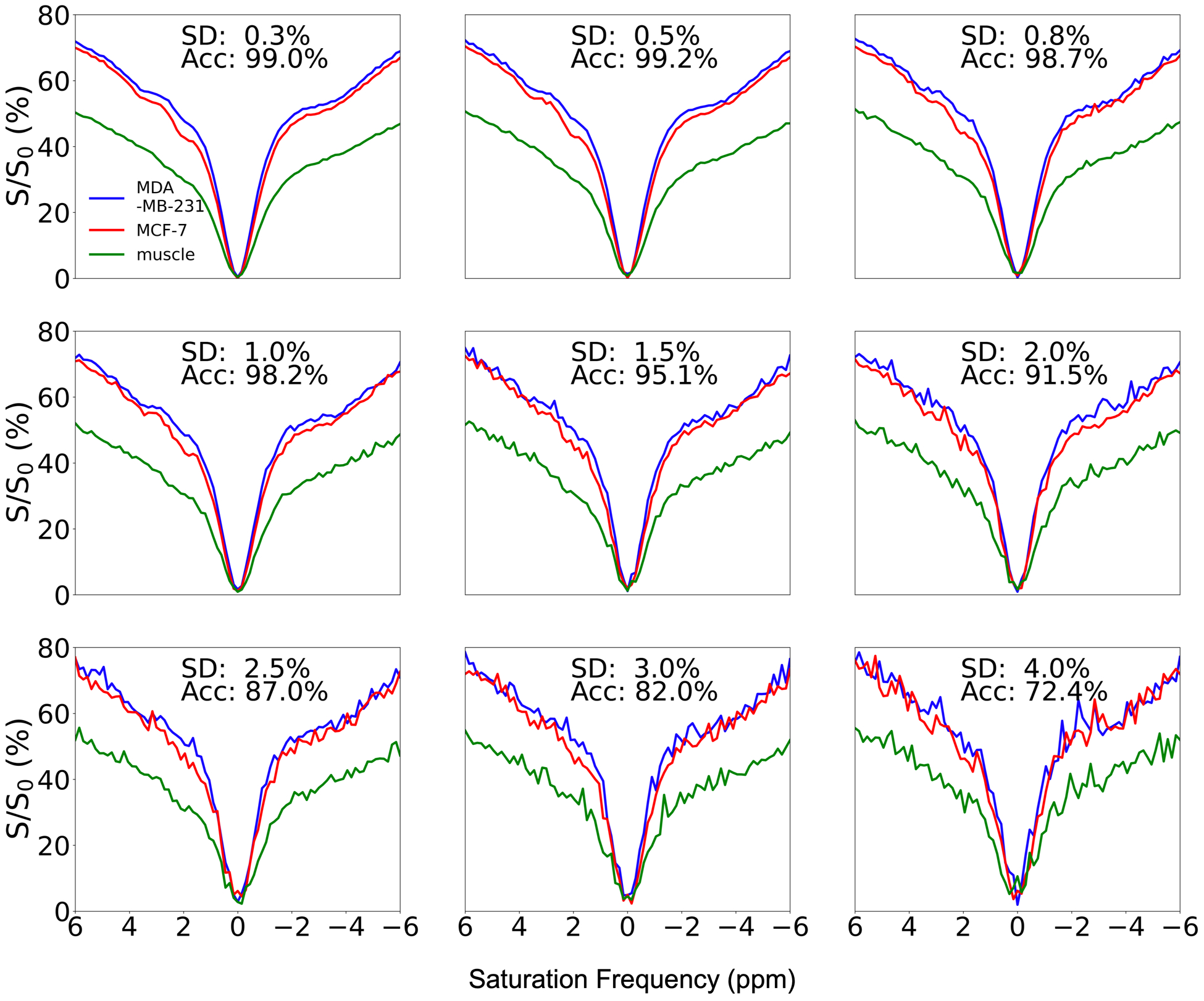
Effects of added noise on classification model performance at B_1,sat = 2.0 μT. The standard deviation (SD) of noise and accuracy of classification are shown in the top center of each subplot.

3.3. Conventional analysis results

LD and MTR_asym analysis were applied to quantify CEST contrast of in vivo data at B_1,sat = 2.0 μT as shown in Figure 4 (data from Mouse #1, which was used for fitting). The T_2w image (Figure 4E) shows a bi-lateral human tumor xenograft mouse with MDA-MB-231 on the right flank (shown in blue) and MCF-7 on the left (shown in red). In Figure 4A, the LD spectral curves of the three tissue types show the mentioned peaks (2.0, 3.5, and −3.5 ppm) in Z-spectra (Figure 2), and the corresponding images at these frequencies (Figure 4C) show that LD can separate tumor from muscle tissue, but cannot distinguish between the tumors. The presence of asymmetric MTC and other up-field signals complicates interpretation of the MTR_asym spectra (Figure 4B), but the MTR_asym spectra of the ROIs seemed to indicate separation of all three tissues in the 3.0 – 4.5 ppm offset range. However, this was not the case on a voxel-by-voxel basis for the complete tumor, where the contrast was heterogeneous. Thus, it was difficult to reliably distinguish between MDA-MB-231 and MCF-7 based on LD and MTR_asym maps in this mouse.

Figure 4.

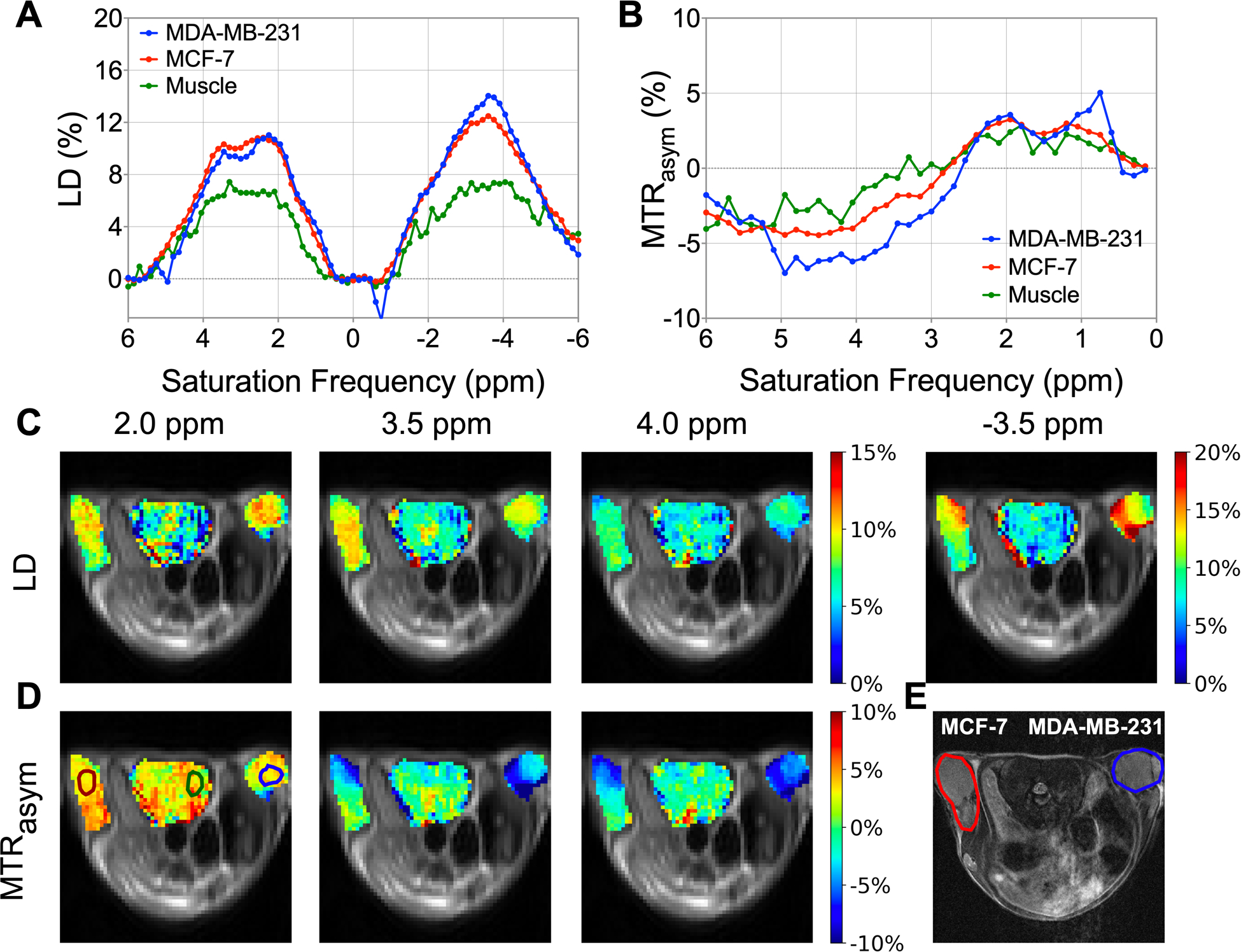
Lorentzian difference (LD) and magnetization transfer ratio asymmetry (MTR_asym) analysis of in vivo data at B_1,sat = 2.0 μT for Mouse #1. (A) LD spectra, and (B) MTR_asym spectra of MDA-MB-231, MCF-7, and muscle tissue. ROIs for the three tissues are indicated in MTR_asym map at 2.0 ppm. (C) LD maps at 2.0, 3.5, 4.0 and −3.5 ppm. (D) MTR_asym maps at 2.0, 3.5, and 4.0 ppm. (E) T_2w image, with MDA-MB-231 shown in blue and MCF-7 shown in red.

Figure 5 summarizes the LD and MTR_asym analysis at specific saturation frequencies (2.0, 3.5, 4.0, and −3.5 ppm) at B_1,sat = 2.0 μT for all mice (ROIs were drawn over known regions of the three tissue types, shown in colored voxels in Figure 4, 6). LD and MTR_asym analysis were first applied on ROIs (Figures 5A–D). LD and MTR_asym spectra with small SD show good reproducibility among these mice (Figures 5A, B). LD intensities between MDA-MB-231 and MCF-7 were only statistically different at −3.5 ppm (Figure 5C), and the MTR_asym intensities between two tumor types were only statistically different at 3.5 ppm (Figure 5D). From both LD and MTR_asym analysis, muscle tissue and two tumor types were statistically different at certain specific saturation frequencies. Furthermore, the histograms for LD and MTR_asym intensities of voxels within ROIs are shown in Figures 5E, F. LD intensities of tumors and muscle tissue were distinguishable but the histograms for MDA-MB-231 and MCF-7 almost completely overlapped. MTR_asym intensities of the three tissues closely resemble each other. Therefore, LD and MTR_asym analysis were unable to classify all three tissue types voxel-by-voxel at these specific saturation frequencies.

Figure 5.

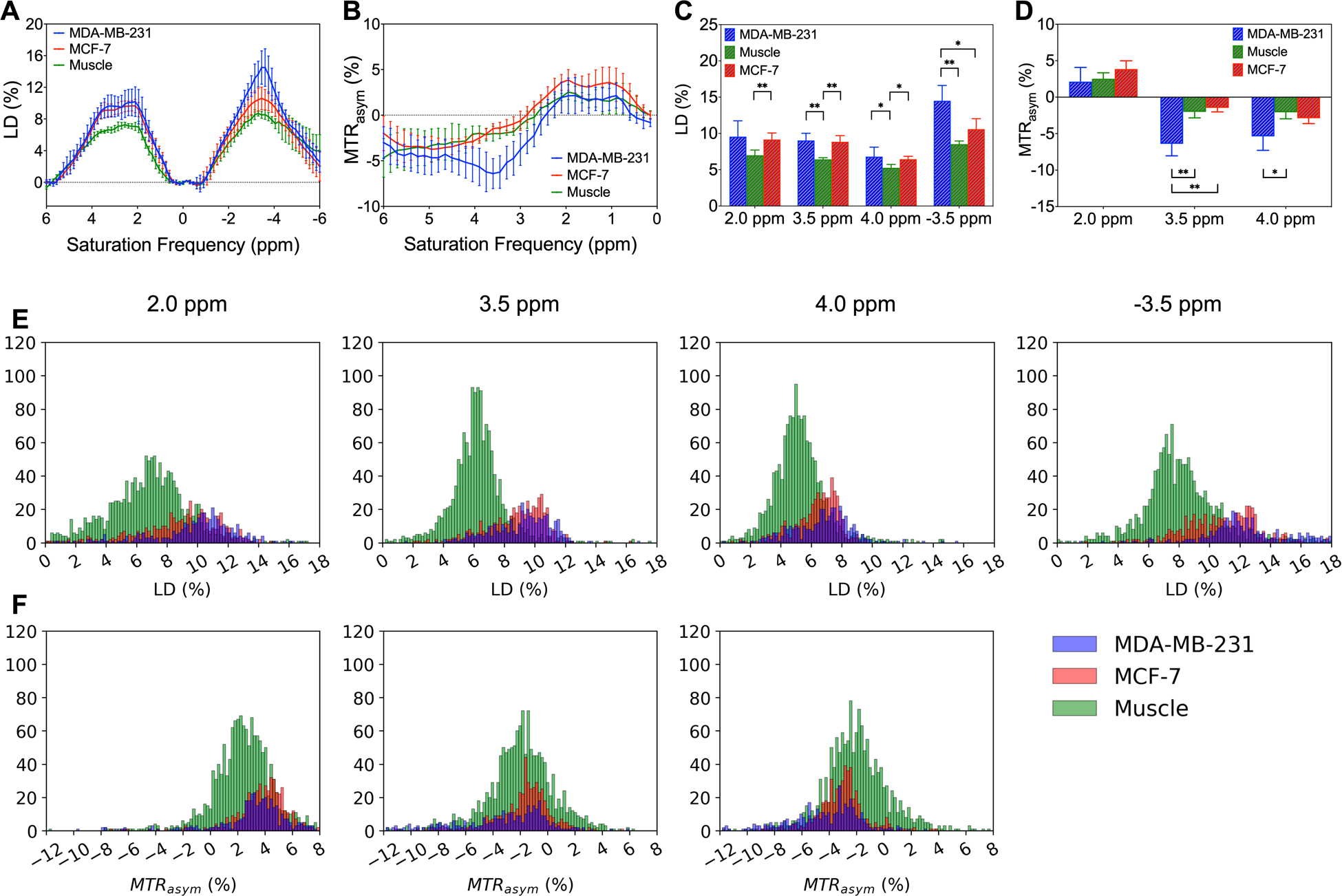
LD and MTR_asym analysis for MDA-MB-231, MCF-7, and muscle tissue at B_1,sat = 2.0 μT. Average and standard deviation of (A) LD and (B) MTR_asym spectra of ROIs. Distributions of (C) LD and (D) MTR_asym of ROIs at specific saturation frequencies (2.0, 3.5, 4.0, and −3.5 ppm) for the three tissue types. Significance levels: *P ≤ 0.05, **P ≤ 0.01. Histograms of (E) LD and (F MTR_asym intensities of voxels within ROIs at these specific frequencies for the three tissue types.

Figure 6.

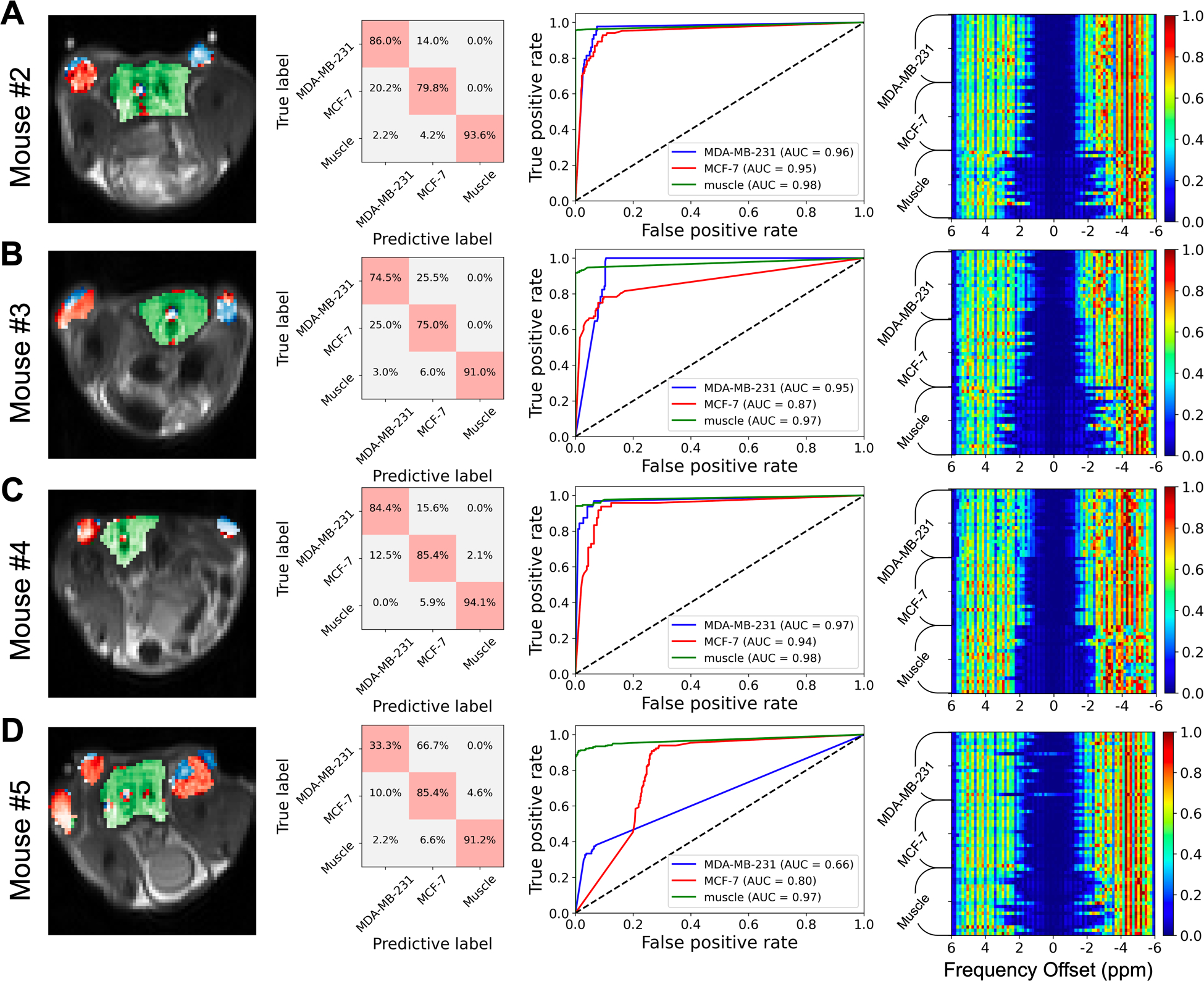
Classification results of the model at B_1,sat = 2.0 μT, using mice #2–5 as testing subjects. Voxels within ROIs (i.e. the colored voxels in the left column) were chosen and labelled for MDA-MB-231, MCF-7, and muscle tissue to evaluate the performance of the classification model. First column, predictive maps (predicted voxels of MDA-MB-231 in blue, MCF-7 in red, and muscle tissue in green); second column, confusion matrix representations; third column, ROC analyses of the prediction performance of the classification model; fourth column, saliency maps of the model.

3.4. Performance of the classification model

Next, the classification model, which was trained using Z-spectral simulations at B_1,sat = 2.0 μT, was tested on the in vivo data to distinguish between the three tissue types on a voxel-wise basis (Figure 6). Mice #2–5 were used as testing subjects. The model performance was evaluated using the voxels within ROIs corresponding to the three tissue types (the colored voxels in Figure 6). To display the classification results intuitively, the predictive results were fused on CEST images (first column, Figure 6). The predictive maps illustrate that the three tissue types could essentially be distinguished, but some voxels were misclassified when the Z-spectra in these false predictive regions closely resembled each other, especially for Mouse #5 (Figure S10). The calculated confusion matrices (second column, Figure 6) showed that the mean true positive (TP) rates of MDA-MB-231, MCF-7, and muscle were 69.6%, 81.4%, and 92.5%, respectively. Additionally, the model provided AUC of the ROCs (third column, Figure 6) with true positive rates ranging from 0.86 to 0.98 for each tissue type classification, indicating good classification efficiency for Mouse #2–4. According to the saliency maps (fourth column, Figure 6), the Z-spectral features between −1.5 to 1.5 ppm were of less importance for classification.

The performance of the classification model using Z-spectra at different B_1,sat levels is shown in Figure 7. The classification model at high B_1,sat (2.0 μT) provided a mean accuracy of 85.7%, sensitivity of 81.1%, and specificity of 94.0% over the tested mice (Figures 7A–C). The model at moderate B_1,sat (1.0 μT) also could distinguish between the three tissue types (mean accuracy of 87.4%, sensitivity of 79.4%, and specificity of 94.1%). However, the Z-spectral features at low B_1,sat (0.5 μT) could not separate two tumor types from muscle tissue (Figures 7D–F). After combining Z-spectral information at multi- B_1,sat (2.0 μT + 1.0 μT, 2.0 μT + 0.5 μT, 1.0 μT + 0.5 μT, and 2.0 μT + 1.0 μT + 0.5 μT), the accuracy, sensitivity, and specificity of classification models changed slightly, and the TP rates were maintained for tumors. Therefore, the performance of model was not improved substantially when using combined CEST data acquired at various B_1,sat.

Figure 7.

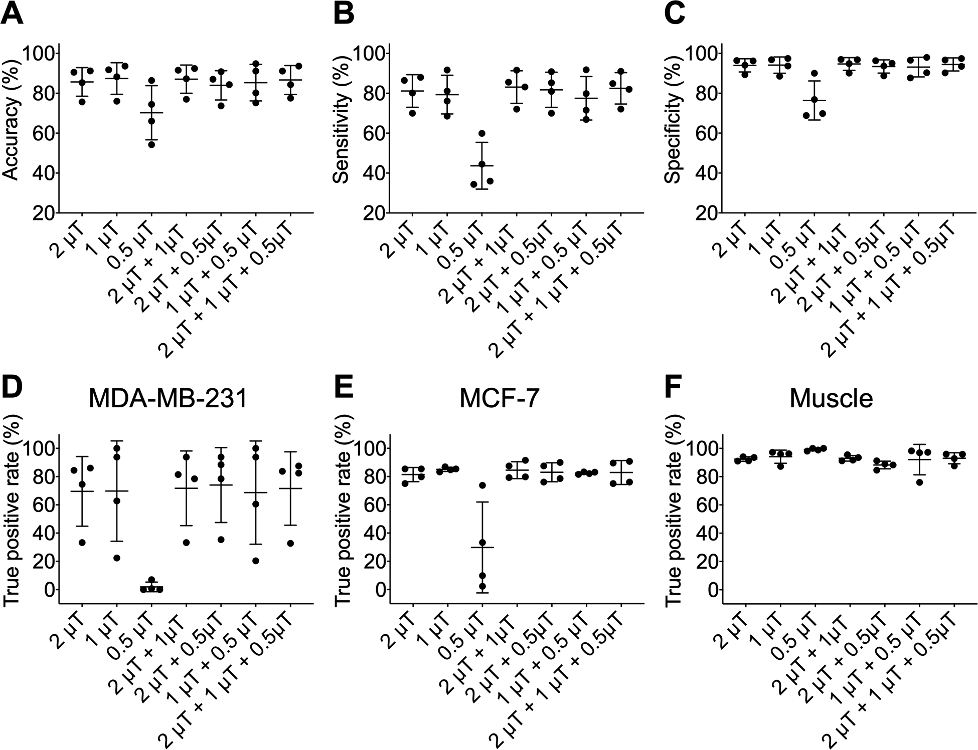
Performance of the classification model using CEST Z-spectra with various saturation pulse amplitude combinations. (A) Accuracy, (B) sensitivity, and (C) specificity of classification model which was training and testing using CEST Z-spectra with B_1,sat = 2.0 μT, 1.0 μT, 0.5 μT, 2.0 μT + 1.0 μT, 2.0 μT + 0.5 μT, 1.0 μT + 0.5 μT, and 2.0 μT + 1.0 μT + 0.5 μT. True positive (TP) rates for (D) MDA-MB-231, (E) MCF-7, and (F) muscle tissue of classification model at different B_1,sat combination.

Then, the influence of LD or MTR_asym spectral features on the performance of classification model at B_1,sat = 2.0 μT was investigated in Figure 8. After combining Z-spectra with LD or MTR_asym spectra, the performance of models did not change within error (mean accuracies of 85.9% and 85.6%, respectively), and the same was true for the TP rates of three tissues types (Figures 8D–F). Therefore, the LD and MTR_asym spectral information did not improve classification performance.

Figure 8.

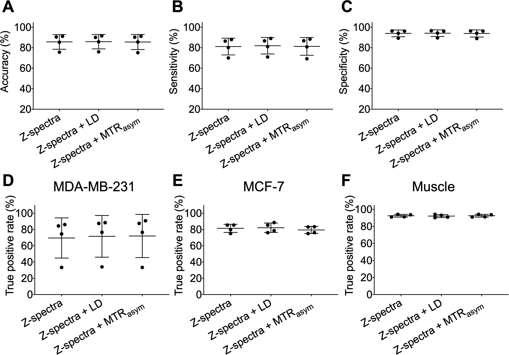
Performance of the classification model at B_1,sat = 2.0 μT using different spectral combinations. (A) Accuracy, (B) sensitivity, and (C) specificity of classification model which was training and testing using Z-spectra, Z-spectra and LD spectra, and Z-spectra and MTR_asym spectra. True positive (TP) rates for (D) MDA-MB-231, (E) MCF-7, and (F) muscle tissue of classification model with different spectral combinations.

Finally, the number of saturation frequencies required for the classification model at B_1,sat = 2.0 μT was assessed in Figure 9. According to saliency maps (Figures 1, 6), the Z-spectral region from −1.5 to 1.5 ppm contributed less to the classification of three tissue types compared to other Z-spectral regions (saliency values close to 0). The model using partial Z-spectra without −1.5 to 1.5 ppm was investigated (totally 62 offsets). To further study the influence of downsampling on the classification model, every second point in the Z-spectra was removed and the region from −1.5 to 1.5 ppm was excluded (totally 32 offsets). Compared with the classification results from the fully sampled Z-spectra with 81 offsets, the performance of model trained with partial or downsampled Z-spectra was maintained (mean accuracies of 85.1% and 85.8%, respectively), and the TP rates of three tissue types only changed slightly when using partial or downsampled Z-spectra. Therefore, Z-spectra can be sampled more sparsely based on saliency maps to reduce acquisition time.

Figure 9.

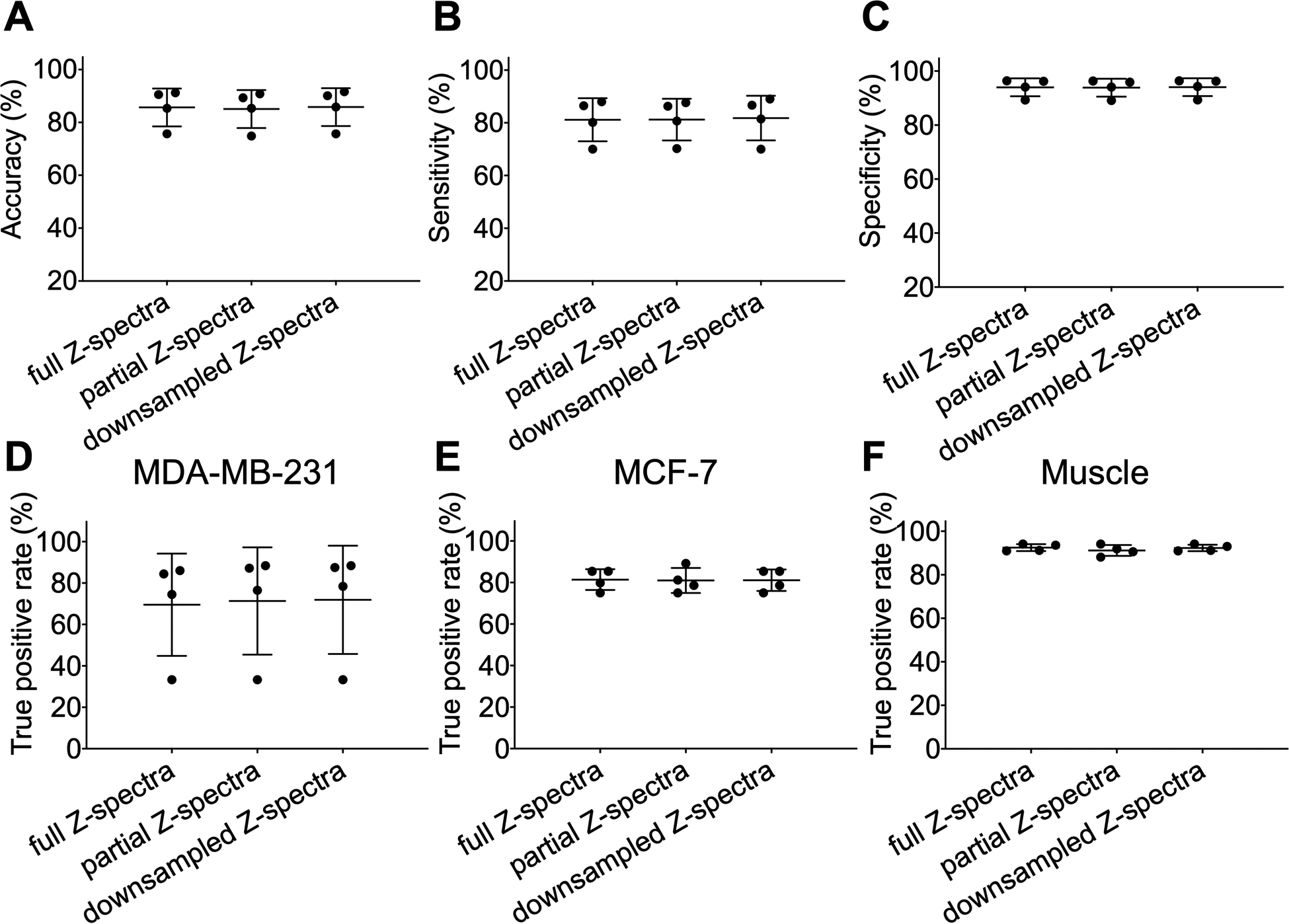
Performance of the classification model at B_1,sat = 2.0 μT using different numbers of saturation frequencies. Partial Z-spectra were chosen without spectral region from −1.5 to 1.5 ppm (total of 62 offsets). Z-spectra were downsampled by collecting every second frequency and excluding −1.5 to 1.5 ppm (total of 32 offsets). (A) Accuracy, (B) sensitivity, and (C) specificity of classification model which was training and testing using partial and downsampled CEST Z-spectra. True positive (TP) rates for (D) MDA-MB-231, (E) MCF-7, and (F) muscle tissue of the classification model with different numbers of saturation frequencies.

4. DISCUSSION

In this study, we developed a CNN-based classification method for processing CEST MRI data and distinguishing different types of tumors. Machine learning-based classification has previously been shown to be useful for classifying Z-spectra of pancreatic tumors²⁵ and here we demonstrated the utility of deep learning to discriminate higher aggressive and lower aggressive tumors and muscle tissue.

When comparing the CNN-based classification model with the fully connected neural network and other machine learning models (e.g., K Nearest Neighbors, Random Forest, Support Vector Machine, and Logistic Regression) at B_1,sat = 2.0 μT, the CNN model was found to slightly outperform other models (Table S4). Still, traditional machine learning models and the DNN model may have higher performance in other situations. In this classification problem, the training data and general structure of the learning model are more important than the specific architecture of model. So while we chose 1D spectral CNN, other models may perform better in other situations. In general, the chosen model should have sufficient abilities to learn the available correlations between the input data and provide a means to visualize the classification (e.g., via saliency maps) to understand and interpret the classification mechanisms and guide downsampling of Z-spectra.

Similar to other deep learning-based classification schemes, the proposed classification approach is data-driven and its performance highly depends on the training data. In this study, three classes of training data were generated using Bloch equations with consideration for differences in the relative concentration of different Z-spectral components in three tissue types. It is worth noting that the parameters used for generating simulation data are not real ground truth values. Here, only the dominant CEST components were considered. Z-spectral peaks acquired with high and moderate B_1,sat were broad and thus were fit well by a single line while peaks in Z-spectra acquired with low B_1,sat were narrow and separated and not fit as well with the limited number of pools (Figure 2), which might cause the poor classification performance at low B_1,sat (Figure 7). However, the tumor size was relatively small, and obtaining a large number of animal datasets for training the deep learning model was not feasible in our study and difficult in general. Previous studies³⁰ along with the present study demonstrate that simulated spectra comprising dominant signal components reasonable concentration ranges can be used as an alternative to the real data and still obtain good performance. The accuracy could be further improved if more in vivo data were available for training. Additionally, through cross-validation, it was found that the classification model was independent of inter-mouse variability (Figure S9).

The performance of the classification model was tested on a synthesized testing dataset and bi-lateral human breast tumor xenograft models. According to the simulations, the model tolerated low and moderate levels of noise but accuracy was reduced at high noise levels (Figure 3), illustrating that the model performance was affected by the quality of input data. Hence, a median filter was applied to improve SNR of in vivo data (Figure S3, Table S2) and further increased the classification performance (Table S1). The in vivo data resembled the simulations with SD of noise around 2.0%, which corresponds to moderate noise levels in the simulations (Tables S2, S3). However, in vivo data was more complex than simulations due to heterogeneity and partial volume effects in tumors, and blood vessels within muscles. Consequently, the classification results from simulations were higher than in vivo data despite similar noise levels. In addition, motion artifacts would interfere in vivo data, especially for tissue boundaries. The in-plane motion of tumors and muscle tissue were relatively small (within 0.2 mm and 0.2°) in dominant Z-spectral classification region (Figure S1), which should have a small impact on classification. However, there was a slight through-plane respiration motion during acquisition that was difficult to correct and thus might affect classification performance. B_1,sat inhomogeneity can also affect CEST data. B_1,sat over the field of view were generated using a PBS phantom and Bloch equation fitting at B_1,sat = 0.5 μT. The map shows that B_1,sat homogeneity was within ±0.1 μT and this variation has only a very slight influence on Z-spectra (Figure S2) thus B_1,sat inhomogeneity was not considered by our models.

The classification model at B_{1, sat} = 2.0 μT could separate the three tissue types voxel-by-voxel but there were still some misclassified voxels that were caused by overlapping Z-spectra with other tissue types (Figure S10). The misclassified tumor voxels were located primarily at the periphery of the tumors, indicating the negative influence of partial volume effects which were possibly exacerbated by motion (Figure 6). And the severe misclassification of MDA-MB-231 for Mouse #5 might be due to tumor heterogeneity which was not considered in the simulated training data. In addition, misclassified muscle tissue might be due to blood vessels. In contrast to the classification model, LD and MTR_asym analysis at specific frequencies were less able to distinguish between the two tumor types at all three B_1,sat amplitudes (Figures 4, 5, S4–S7). Therefore, the classification model had superior ability to distinguish between different tumors and potentially could be used on a voxel-wise basis to study different tumor regions.

The CNN model could provide saliency maps (Figures 1, 6). According to saliency maps of CNN at B_1,sat = 2.0 μT, the Z-spectral region from −1.5 to 1.5 ppm (dominated by the direct water saturation signal) had little impact on the classification, showing that the classification was primarily based on the relative concentrations of the different Z-spectral components but not the tissue water relaxation properties. This was also observed from the fitted set of Bloch equation parameters which showed the Z-spectra of the tissue types clearly differed from each other in the relative concentration of Z-spectral components, especially MTC (Table 1). In addition, the saliency maps illustrate that compared to the easily identifiable muscle tissue, the model required more Z-spectral features to distinguish between the two tumor types which were difficult to separate.

The inclusion of additional CEST data and parameters in the classification model was assessed to determine if they improve classification performance. The combination of features at multi-B_1,sat did not improve classification performance (Figure 7), illustrating that there was redundant information in the combination input features. It was also intuitive that the model performance remained unchanged when using additional LD or MTR_asym spectra (Figure 8) since LD and MTR_asym are different representations of the same CEST information contained in Z-spectra, and would be regarded as redundant information in classification model.

It is also important to consider how the classification model performs with more sparely sampled data which can greatly speed up acquisition. Saliency maps guided the downsampling of Z-spectra and the performance of the model with saliency map-based partial or downsampled Z-spectra was surprisingly maintained (Figure 9). This suggests that only pertinent spectral regions or sparsely-sampled Z-spectra may be needed for tumor detection and classification, which will allow much shorter CEST acquisitions without compromising diagnostic efficacy. In this sampling scheme, excluding Z-spectral regions did not dramatically affect B₀ correction (Figure S11). Further refinement of the saturation frequency list may be possible, especially based on the approach presented in this work, and perhaps also using different intervals between frequencies for different parts of the spectrum.

Finally, the proposed classification model can be easily tailored to other cancer types beyond breast cancer. The Z-spectra of various tissue types in the brain and body could be analyzed using the proposed approach to achieve classification of different tissue types.

However, the limitation of the present study is that the performance of classification model might be affected by simulated training data based on a limited number of pools, which might not represent the ground truth. Nevertheless, the present study demonstrates a proof-of-concept study to utilize the ability of deep learning with simulated training data to analyze tissue-specific Z-spectra for accurate tissue classification. Additionally, the Z-spectra acquired at higher magnetic fields (11.7 T) will have more clearly resolved features, which is helpful for the current deep learning classification model. Accordingly, the models may not work well on data acquired at lower magnetic fields.

In summary, we demonstrated the capability of a CNN-based classification model to distinguish between multiple tissue types based on their Z-spectral features. The performance of classification was robust in the presence of low and moderate noise perturbations and did not substantially change when including additionally spectral features. The model also produced saliency maps revealing pertinent regions on the Z-spectra which could be used to speed up CEST acquisition protocols by sampling limited frequencies. The method could classify in vivo tumors and muscle tissue voxel-by-voxel, implying deep learning technologies have potential to be helpful for utilizing and interpreting CEST spectral data.

ABBREVIATIONS

ANN

artificial neural network

AUC

area under curve

CEST

chemical exchange saturation transfer

CNN

convolutional neural network

CW

continuous-wave

Cr

Creatine

DS

direct water saturation

FN

false negative

FOV

field of view

FP

false positive

LD

Lorentzian difference

MRI

magnetic resonance imaging

MTC

magnetization transfer contrast

MTR_asym

magnetization transfer ratio asymmetry

PBS

phosphate‐buffered saline

PCA

principal component analysis

PCr

phosphocreatine

rNOEs

relayed Nuclear Overhauser Effects

RARE

rapid acquisition with relaxation enhancement

ROC

receiver operating curve

ROIs

regions of interests

SD

standard deviation

SNR

signal-to-noise

T2_w

T2-weighted

TP

true positive

TN

true negative

DATA AVAILABILITY STATEMENT

All materials are available on request, imaging data and analysis code can be downloaded from a public repository, https://github.com/ChongxueBie/Classification_Breast_Tumors.git

References

- 1.van Zijl PCM, Yadav NN. Chemical exchange saturation transfer (CEST): What is in a name and what isn’t? Magn Reson Med. 2011;65:927–948. [DOI] [PMC free article] [PubMed] [Google Scholar]
- 2.Zhou J, Lal B, Wilson DA, Laterra J, van Zijl PCM. Amide proton transfer (APT) contrast for imaging of brain tumors. Magn Reson Med. 2003;50:1120–1126. [DOI] [PubMed] [Google Scholar]
- 3.Jones CK, Schlosser MJ, van Zijl PCM, Pomper MG, Golay X, Zhou J. Amide proton transfer imaging of human brain tumors at 3T. Magn Reson Med. 2006;56:585–592. [DOI] [PubMed] [Google Scholar]
- 4.Zhou IY, Wang E, Cheung JS, Zhang X, Fulci G, Sun PZ. Quantitative chemical exchange saturation transfer (CEST) MRI of glioma using Image Downsampling Expedited Adaptive Least-squares (IDEAL) fitting. Sci Rep. 2017;7:84. [DOI] [PMC free article] [PubMed] [Google Scholar]
- 5.Chan KW, Jiang L, Cheng M, et al. CEST-MRI detects metabolite levels altered by breast cancer cell aggressiveness and chemotherapy response. NMR Biomed. 2016;29:806–816. [DOI] [PMC free article] [PubMed] [Google Scholar]
- 6.Jia G, Abaza R, Williams JD, et al. Amide proton transfer MR imaging of prostate cancer: A preliminary study. J Magn Reson Imaging. 2011;33:647–654. [DOI] [PMC free article] [PubMed] [Google Scholar]
- 7.Zhou J, Heo H-Y, Knutsson L, van Zijl PCM, Jiang S. APT-weighted MRI: Techniques, current neuro applications, and challenging issues. J Magn Reson Imaging. 2019;50:347–364. [DOI] [PMC free article] [PubMed] [Google Scholar]
- 8.Chen M, Chen C, Shen Z, et al. Extracellular pH is a biomarker enabling detection of breast cancer and liver cancer using CEST MRI. Oncotarget. 2017;8:45759–45767. [DOI] [PMC free article] [PubMed] [Google Scholar]
- 9.Zaric O, Farr A, Poblador Rodriguez E, et al. 7T CEST MRI: A potential imaging tool for the assessment of tumor grade and cell proliferation in breast cancer. Magn Reson Med. 2019;59:77–87. [DOI] [PubMed] [Google Scholar]
- 10.Dula AN, Dewey BE, Arlinghaus LR, et al. Optimization of 7-T chemical exchange saturation transfer parameters for validation of glycosaminoglycan and amide proton transfer of fibroglandular breast tissue. Radiology. 2015;275:255–261. [DOI] [PMC free article] [PubMed] [Google Scholar]
- 11.Klomp DWJ, Dula AN, Arlinghaus LR, et al. Amide proton transfer imaging of the human breast at 7T: development and reproducibility. NMR Biomed. 2013;26:1271–1277. [DOI] [PMC free article] [PubMed] [Google Scholar]
- 12.Dula AN, Arlinghaus LR, Dortch RD, et al. Amide proton transfer imaging of the breast at 3 T: establishing reproducibility and possible feasibility assessing chemotherapy response. Magn Reson Med. 2013;70:216–224. [DOI] [PMC free article] [PubMed] [Google Scholar]
- 13.Chan KW, McMahon MT, Kato Y, et al. Natural D-glucose as a biodegradable MRI contrast agent for detecting cancer. Magn Reson Med. 2012;68:1764–1773. [DOI] [PMC free article] [PubMed] [Google Scholar]
- 14.Jones KM, Pollard AC, Pagel MD. Clinical applications of chemical exchange saturation transfer (CEST) MRI. J Magn Reson Imaging. 2018;47:11–27. [DOI] [PMC free article] [PubMed] [Google Scholar]
- 15.Dula AN, Smith SA, Gore JC. Application of chemical exchange saturation transfer (CEST) MRI for endogenous contrast at 7 Tesla. J Neuroimaging. 2013;23:526–532. [DOI] [PMC free article] [PubMed] [Google Scholar]
- 16.Zhang X-Y, Wang F, Xu J, Gochberg DF, Gore JC, Zu Z. Increased CEST specificity for amide and fast-exchanging amine protons using exchange-dependent relaxation rate. NMR Biomed. 2018;31: 10.1002/nbm.3863. [DOI] [PMC free article] [PubMed] [Google Scholar]
- 17.Zu Z, Janve VA, Li K, Does MD, Gore JC, Gochberg DF. Multi-angle ratiometric approach to measure chemical exchange in amide proton transfer imaging. Magn Reson Med. 2012;68:711–719. [DOI] [PMC free article] [PubMed] [Google Scholar]
- 18.Jones CK, Huang A, Xu J, et al. Nuclear Overhauser enhancement (NOE) imaging in the human brain at 7T. NeuroImage. 2013;77:114–124. [DOI] [PMC free article] [PubMed] [Google Scholar]
- 19.Ling W, Regatte RR, Navon G, Jerschow A. Assessment of glycosaminoglycan concentration in vivo by chemical exchange-dependent saturation transfer (gagCEST). Proc Natl Acad Sci U S A. 2008;105:2266–2270. [DOI] [PMC free article] [PubMed] [Google Scholar]
- 20.van Zijl PCM, Zhou J, Mori N, Payen J-F, Wilson D, Mori S. Mechanism of magnetization transfer during on-resonance water saturation. A new approach to detect mobile proteins, peptides, and lipids. Magn Reson Med. 2003;49:440–449. [DOI] [PubMed] [Google Scholar]
- 21.Xu J, Zaiss M, Zu Z, et al. On the origins of chemical exchange saturation transfer (CEST) contrast in tumors at 9.4 T. NMR Biomed. 2014;27:406–416. [DOI] [PMC free article] [PubMed] [Google Scholar]
- 22.Akkus Z, Galimzianova A, Hoogi A, Rubin DL, Erickson BJ. Deep Learning for Brain MRI Segmentation: State of the Art and Future Directions. J Digit Imaging. 2017;30:449–459. [DOI] [PMC free article] [PubMed] [Google Scholar]
- 23.Lee HH, Kim H. Intact metabolite spectrum mining by deep learning in proton magnetic resonance spectroscopy of the brain. Magn Reson Med. 2019;82:33–48. [DOI] [PubMed] [Google Scholar]
- 24.Usman K, Rajpoot K. Brain tumor classification from multi-modality MRI using wavelets and machine learning. Pattern Anal Appl. 2017;20:871–881. [Google Scholar]
- 25.Goldenberg JM, Cardenas-Rodriguez J, Pagel MD. Machine learning improves classification of preclinical models of pancreatic cancer with chemical exchange saturation transfer MRI. Magn Reson Med. 2019;81:594–601. [DOI] [PMC free article] [PubMed] [Google Scholar]
- 26.LeCun Y, Bengio Y, Hinton G. Deep learning. Nature. 2015;521:436–444. [DOI] [PubMed] [Google Scholar]
- 27.Schmidhuber J Deep learning in neural networks: An overview. Neural Netw. 2015;61:85–117. [DOI] [PubMed] [Google Scholar]
- 28.Zaiss M, Deshmane A, Schuppert M, et al. DeepCEST: 9.4 T Chemical exchange saturation transfer MRI contrast predicted from 3 T data - a proof of concept study. Magn Reson Med. 2019;81:3901–3914. [DOI] [PubMed] [Google Scholar]
- 29.Glang F, Deshmane A, Prokudin S, et al. DeepCEST 3T: Robust MRI parameter determination and uncertainty quantification with neural networks—application to CEST imaging of the human brain at 3T. Magn Reson Med. 2020;84:450–466. [DOI] [PubMed] [Google Scholar]
- 30.Chen L, Schar M, Chan KWY, et al. In vivo imaging of phosphocreatine with artificial neural networks. Nat Commun. 2020;11:1072. [DOI] [PMC free article] [PubMed] [Google Scholar]
- 31.Kim M, Gillen J, Landman BA, Zhou J, van Zijl PCM. Water saturation shift referencing (WASSR) for chemical exchange saturation transfer (CEST) experiments. Magn Reson Med. 2009;61:1441–1450. [DOI] [PMC free article] [PubMed] [Google Scholar]
- 32.Zaiss M, Zu Z, Xu J, et al. A combined analytical solution for chemical exchange saturation transfer and semi-solid magnetization transfer. NMR Biomed. 2015;28:217–230. [DOI] [PMC free article] [PubMed] [Google Scholar]
- 33.Nash JE, Sutcliffe JV. River flow forecasting through conceptual models part I — A discussion of principles. J Hydrol. 1970;10:282–290. [Google Scholar]
- 34.Guivel-Scharen V, Sinnwell T, Wolff SD, Balaban RS. Detection of Proton Chemical Exchange between Metabolites and Water in Biological Tissues. J Magn Reson. 1998;133:36–45. [DOI] [PubMed] [Google Scholar]
- 35.Zhou J, van Zijl PCM. Chemical exchange saturation transfer imaging and spectroscopy. Prog Nucl Magn Reson Spectrosc. 2006;48:109–136. [Google Scholar]
- 36.van Zijl PCM, Lam WW, Xu J, Knutsson L, Stanisz GJ. Magnetization Transfer Contrast and Chemical Exchange Saturation Transfer MRI. Features and analysis of the field-dependent saturation spectrum. Neuroimage. 2018;168:222–241. [DOI] [PMC free article] [PubMed] [Google Scholar]
- 37.Tietze A, Blicher J, Mikkelsen IK, et al. Assessment of ischemic penumbra in patients with hyperacute stroke using amide proton transfer (APT) chemical exchange saturation transfer (CEST) MRI. NMR Biomed. 2014;27:163–174. [DOI] [PMC free article] [PubMed] [Google Scholar]
- 38.Zhang X-Y, Wang F, Li H, et al. Accuracy in the quantification of chemical exchange saturation transfer (CEST) and relayed nuclear Overhauser enhancement (rNOE) saturation transfer effects. NMR Biomed. 2017;30:e3716. [DOI] [PMC free article] [PubMed] [Google Scholar]
- 39.Zaiss M, Schmitt B, Bachert P. Quantitative separation of CEST effect from magnetization transfer and spillover effects by Lorentzian-line-fit analysis of z-spectra. J Magn Reson. 2011;211:149–155. [DOI] [PubMed] [Google Scholar]
- 40.Liu G, Gilad AA, Bulte JWM, van Zijl PCM, McMahon MT. High-throughput screening of chemical exchange saturation transfer MR contrast agents. Contrast Media Mol Imaging. 2010;5:162–170. [DOI] [PMC free article] [PubMed] [Google Scholar]
- 41.Zaiss M CEST sources. http://www.cest sources.org. Published 2014. Accessed September 1, 2020.
- 42.Gudbjartsson H, Patz S. The rician distribution of noisy mri data. Magn Reson Med. 1995;34:910–914. [DOI] [PMC free article] [PubMed] [Google Scholar]
- 43.Bottou L Large-scale machine learning with stochastic gradient descent. In: Proceedings of COMPSTAT’2010. Springer; 2010:177–186. [Google Scholar]
- 44.Simonyan K, Vedaldi A, Zisserman A. Deep inside convolutional networks: Visualising image classification models and saliency maps. arXiv preprint arXiv:13126034. 2013. [Google Scholar]
- 45.Chollet F. Keras. https://github.com/fchollet/keras. Published 2015. Accessed October 1, 2020.
- 46.Abadi M, Barham P, Chen J, et al. TensorFlow: a system for large-scale machine learning. Proceedings of the 12th USENIX conference on Operating Systems Design and Implementation; 2016; Savannah, GA, USA. [Google Scholar]
- 47.Kotikalapudi Raghavendra. keras-vis. GitHub. https://github.com/raghakot/keras-vis. Published 2017. Accessed February 1, 2021. [Google Scholar]
Associated Data
This section collects any data citations, data availability statements, or supplementary materials included in this article.
Supplementary Materials