Differential Effects of Endogenous and Exogenous Attention on Sensory Tuning

Abstract

Covert spatial attention (without concurrent eye movements) improves performance in many visual tasks (e.g., orientation discrimination and visual search). However, both covert attention systems—endogenous (voluntary) and exogenous (involuntary)—exhibit differential effects on performance in tasks mediated by spatial and temporal resolution suggesting an underlying mechanistic difference. We investigated whether these differences manifest in sensory tuning by assessing whether and how endogenous and exogenous attention differentially alter the representation of two basic visual dimensions—orientation and spatial frequency (SF). The same human observers detected a grating embedded in noise in two separate experiments (with endogenous or exogenous attention cues). Reverse correlation was used to infer the underlying neural representation from behavioral responses, and we linked our results to established neural computations via a normalization model of attention. Both endogenous and exogenous attention similarly improved performance at the attended location by enhancing the gain of all orientations without changing tuning width. In the SF dimension, endogenous attention enhanced the gain of SFs above and below the target SF, whereas exogenous attention only enhanced those above. Additionally, exogenous attention shifted peak sensitivity to SFs above the target SF, whereas endogenous attention did not. Both covert attention systems modulated sensory tuning via the same computation (gain changes). However, there were differences in the strength of the gain. Compared with endogenous attention, exogenous attention had a stronger orientation gain enhancement but a weaker overall SF gain enhancement. These differences in sensory tuning may underlie differential effects of endogenous and exogenous attention on performance.

SIGNIFICANCE STATEMENT Covert spatial attention is a fundamental aspect of cognition and perception that allows us to selectively process and prioritize incoming visual information at a given location. There are two types: endogenous (voluntary) and exogenous (involuntary). Both typically improve visual perception, but there are instances where endogenous improves perception but exogenous hinders perception. Whether and how such differences extend to sensory representations is unknown. Here we show that both endogenous and exogenous attention mediate perception via the same neural computation—gain changes—but the strength of the orientation gain and the range of enhanced spatial frequencies depends on the type of attention being deployed. These findings reveal that both attention systems differentially reshape the tuning of features coded in striate cortex.

Introduction

Attention improves visual perception by selectively processing incoming information. Such a system is necessary given the high cost of cortical computation and the constant exposure of our visual system to far more information than it can process (Lennie, 2003). There are the following two types of covert spatial attention: endogenous (voluntary, goal driven, and deployed in ∼300 ms); and exogenous (involuntary, stimulus driven, and deployed fast and transiently, peaking at ∼100 ms; for review, see Carrasco, 2011, 2014). Similar temporal dynamics have been reported from single-cell recordings in macaque area MT (Busse et al., 2008). Orienting covert spatial attention to a target location benefits performance in many tasks. These improvements often manifest via an increase in contrast sensitivity—the ability to distinguish an object from its surroundings—and spatial resolution—the ability to see fine detail (for review, see Carrasco, 2011, 2014; Anton-Erxleben and Carrasco, 2013; Carrasco and Barbot, 2014).

Differences exist in how endogenous and exogenous attention modulate contrast responses. Endogenous attention typically increases contrast sensitivity via a contrast gain (α) change, whereas exogenous attention increases maximal contrast responses via a response gain change (Ling and Carrasco, 2006; Pestilli et al., 2009; Fernández and Carrasco, 2020; but see Morrone et al., 2002, 2004). A prominent normalization model of attention postulates that these differences are because of changes in the size of the attention field relative to the stimulus size (Reynolds and Heeger, 2009).

Differences also exist in tasks mediated by spatial resolution (e.g., texture segmentation). Endogenous attention optimizes resolution to improve performance at central and peripheral locations (Yeshurun et al., 2008; Barbot and Carrasco, 2017; Jigo and Carrasco, 2018). Exogenous attention inflexibly increases resolution, resulting in performance benefits at peripheral locations and costs at central locations (Yeshurun and Carrasco, 1998, 2000; Talgar and Carrasco, 2002). Adapting observers to high spatial frequencies (SFs) removes the attentional impairment, suggesting that exogenous attention inflexibly increases resolution by enhancing sensitivity to high SFs (Carrasco et al., 2006). Endogenous attention improves performance at all eccentricities by flexibly adjusting resolution according to task demands (Barbot and Carrasco, 2017). Given the trade-off between spatial and temporal resolution, exogenous attention enhances spatial resolution but degrades temporal resolution (Yeshurun and Levy, 2003; Yeshurun, 2004; Rolke et al., 2008) and perceived motion (Yeshurun and Hein, 2011). Conversely, endogenous attention improves both spatial and temporal resolution (Sharp et al., 2018).

A recent normalization model of attention reproduces the well established differential effects of endogenous and exogenous attention on contrast sensitivity and spatial resolution; to do so, the model requires that the attention effects be mediated by differences in SF tuning (Jigo et al., 2021). Here, we investigate, for the first time, whether and how endogenous and exogenous attention differentially mediate sensory representations. We focus on two vision building blocks coded in V1: orientation and SF (Hubel and Wiesel, 1959; Maffei and Fiorentini, 1977). Sensory representations were assessed using reverse correlation, which provides a measure of how changes in external noise influence performance, is widely used to probe the mechanisms underlying behavioral responses to noisy stimuli (Ahumada, 1996; Eckstein and Ahumada, 2002; Wyart et al., 2012; Li et al., 2016) and can approximate electrophysiological sensory tuning properties (Neri and Levi, 2006). Here we used (1) signal detection theory to assess humans' performance with endogenous and exogenous attention, (2) reverse correlation to uncover the underlying computations, and (3) a normalization model of attention to link the observed behavioral effects to established neural computations.

The same observers completed two experiments with identical stimuli and tasks but different cues. Both endogenous and exogenous attention altered orientation tuning via a multiplicative gain enhancement without changing tuning width (σ). Critically, endogenous attention enhanced sensitivity to SFs at, above, and below the target SF, whereas exogenous attention preferentially enhanced SFs above the target SF. These findings provide critical empirical evidence for the assumed differential SF profiles required to model the effects of these two types of attention on performance (Jigo et al., 2021).

Materials and Methods

Observers

The same six observers (age range, 19–26 years; four females), including authors A.F. and S.O., participated in both experiments (15 experimental sessions per experiment). All observers had normal or corrected-to-normal vision and provided informed consent. All experimental procedures were in agreement with the Declaration of Helsinki and were approved by the university committee on activities involving human subjects at New York University.

Apparatus

Stimuli were generated using MATLAB (MathWorks) and the Psychophysics toolbox (Brainard, 1997; Pelli, 1997; Kleiner et al., 2007). Observers sat in a dimly lit room with their head positioned on a chinrest 57 cm away from a 22 inch monitor (model Vision Master Pro 514-CRT; resolution, 1280 × 960; 100 Hz). A ColorCAL MKII Colorimeter was used for gamma correction (Cambridge Research Systems). Observers viewed the monitor display binocularly, and fixation was monitored using an EyeLink 1000 Eye Tracker (SR Research) at a sampling rate of 1000 Hz.

Stimuli

Stimuli were presented on a gray background (luminance, 68 cd/m²) at four spatial locations denoted by placeholders composed of four black dots forming a square (3° wide; Fig. 1A). The placeholders remained on the screen for the entire experimental session and were presented at each intercardinal location at 7° of eccentricity. The target was a random-phase vertical Gabor generated by modulating a 2 cycles per degree (cpd) sine wave with a Gaussian envelope (0.8° SD). Four white noise patches were independently and randomly generated on each trial and presented inside each placeholder. The noise was bandpass filtered to contain SFs between 1 and 4 cpd and were scaled to have 0.12 root mean square contrast. On any given trial, the test stimulus could be a noise patch or a target embedded in noise (Fig. 1A,B). The same stimuli were used in both experiments.

Figure 1.

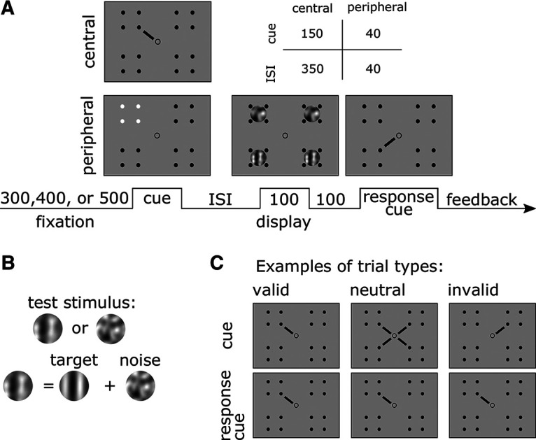
A, Trial timeline in milliseconds. Observers performed two yes/no detection tasks. For endogenous attention (experiment 1), the cue was a line extending from the center indicating one spatial location (central cue). For exogenous attention (experiment 2), the placeholder at one spatial location briefly changed in polarity (peripheral cue). The timing (cue and ISI) differed for both experiments (central and peripheral cue) to optimize the effectiveness of the cues. B, Stimuli. In half of the trials, the test stimulus consisted of a Gabor filter embedded in noise; in the other half, the stimulus was just noise. C, Trial types. The example demonstrates valid, neutral, and invalid trials in experiment 1. In experiment 2, the cue and response cue mappings were the same, but the cue was peripheral instead of central.

Experimental design and statistical analysis

Task procedures

Experiment 1.

Observers performed a visual detection task. A test stimulus, defined as the patch probed by the response cue, was presented at one of four possible spatial locations denoted by placeholders. In half of the trials, the test stimulus contained only noise; in the other half, the target was embedded in the noise. To diminish temporal expectation and ensure our attention effects were driven by the cues, each trial began with one of three equally likely fixation periods (300, 400, or 500 ms). After the fixation period, a precue was presented for 150 ms, followed by a brief interstimulus interval (ISI) of 350 ms. Next, four patches (three irrelevant stimuli and one test stimulus), one inside each placeholder, were simultaneously presented for 100 ms. Each placeholder could encompass a patch composed of a target embedded in the noise or just noise with 50% probability. Thus, on any given trial, whether a target was presented was independently determined for all four locations.

The test stimulus was indicated by a central response cue, which was presented 100 ms after the offset of the patches and remained on the screen until response. The cue validity was manipulated such that 60% of the trials were valid, 20% were neutral, and the remaining 20% were invalid; from the cued trials indicating one location, 75% were valid trials (Fig. 1C). Therefore, observers were incentivized to deploy their voluntary spatial attention to the location probed by the precue as most of the trials were valid. In the valid and invalid trials, the precue was presented as a central line pointing to one of the placeholders. In valid trials, the precue matched the response cue; in invalid trials, the precue and response cue did not match. In neutral trials, all locations were precued (four lines, one pointing to each placeholder) to distribute attention to all placeholders. The observers' task was to detect whether the test stimulus contained a target by pressing the “z” key for yes or “?” for no on an apple keyboard. On incorrect trials, observers received auditory feedback in the form of a tone (400 Hz). At the end of each block, observers also received feedback in the form of percentage correct.

All attention conditions (valid, invalid, and neutral) were interleaved within each block. Observers completed seven blocks for a total of 1008 trials per session. Each observer completed a training session (1008 trials) to familiarize themselves with the task. This was followed by 15 experimental sessions (15,120 sessions). During training, a contrast threshold—defined as the level of contrast needed to achieve 75% accuracy on neutral trials—was determined for the target using an adaptive titration method (Best-PEST; Pentland, 1980).

If an observer was underperforming/overperforming by ≥5% on neutral trials on any given session, their contrast threshold was updated in the following session.

Stimulus presentation was contingent on central fixation. Fixation was monitored from the start of the trial until response cue presentation. Trials with fixation breaks or blinks—defined as a deviation in eye position by ≥1.5° from fixation—were repeated at the end of the block. On average, 5.25% of trials in experiment 1 and 1.58% of trials in experiment 2 were repeated.

Experiment 2.

The task was very similar to experiment 1 with slight differences to facilitate the effects of exogenous attention on performance. The attentional cues changed from central to peripheral (Fig. 1) and were composed of a brief change in polarity of one (valid/invalid) or all (neutral) placeholders, and the duration of the cue and ISI was decreased to 40 ms each (Fig. 1). Cue validity was equated across valid, invalid, and neutral trials (33% for each condition), making the cues uninformative.

Reverse correlation.

Reverse correlation, assuming a general linear model approach (Fig. 2; Ahumada, 1996; Eckstein and Ahumada, 2002; Wyart et al., 2012; Li et al., 2016; Fernández et al., 2019), was used to assess the computations underlying the modulatory effect of attention on performance. The noise image of the test stimulus was transformed from a space defined by pixel luminance intensities to a space defined by the contrast energy across orientation (−80 to 80 with 19 points equally spaced on a linear scale) and SF (from 1 to 4 cpd with 15 points evenly spaced on a log scale) components in the noise. We took the noise images $S$ across trials and convolved them with two Gabor filters $g$ (same size as the target) in quadrature phase with the corresponding orientation $\theta$ and SF $f$ to compute energy $E_{\theta ,f}$ for all components, which is given by the following expression:

$$E_{\theta ,f}=\sqrt{{\left(S\ast g_{\theta ,f,\text{sin}}\right)}^2+{\left(S\ast g_{\theta ,f,\text{cos}}\right)}^2}.$$

Figure 2.

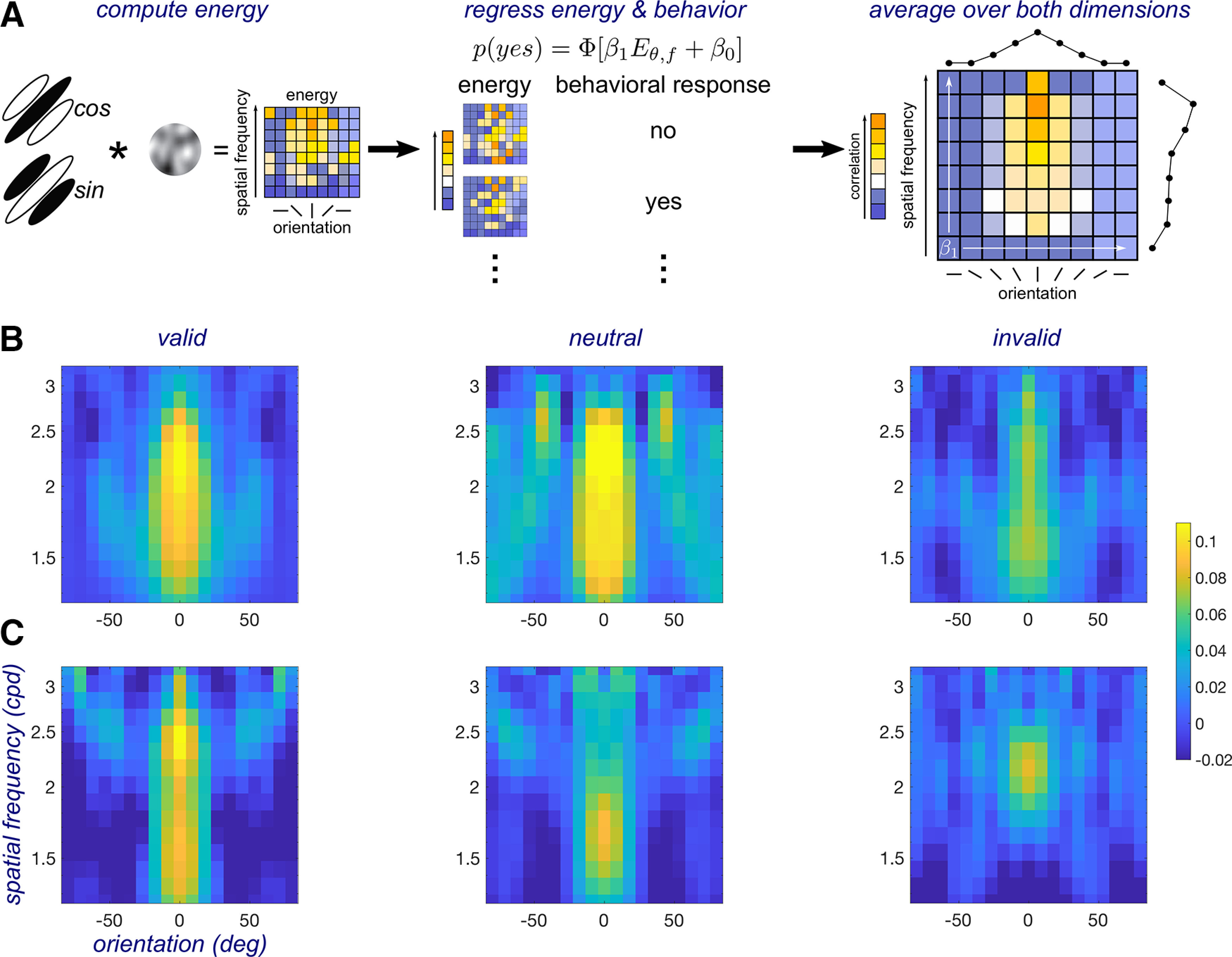
A, Reverse correlation: (1) compute energy by convolving a bank of Gabor filters in quadrature phase with the noise patches; (2) regress the trial-wise energy fluctuations with behavioral responses; and (3) the slope of the regression indexes sensitivity; take the mean (marginals) of the slope across the orientation and SF dimension to compute tuning functions. B, Endogenous attention (experiment 1) kernels for one individual observer. C, Exogenous attention (experiment 2) kernels for the same observer.

We regressed the energy of each component with behavioral responses using probit binomial regression. The regression model was expressed as follows:

$$p(\text{yes})=\Phi [{\beta }_1{E}_{\theta ,f}+{\beta }_0],$$

where ${\beta }_1$ is the slope of the regression and indicates the level of correlation between the energy and behavioral reports, ${\beta }_0$ is an intercept term, and $\Phi$[.] indicates a probit link—inverse of the normal cumulative distribution function. We used the slope to index perceptual sensitivity. A slope of zero indicates that the energy of that component did not influence the observer's responses. Before regressing, the energy of each component was sorted into a present or absent group, and the mean of the energy for each group was subtracted and normalized to have an SD of 1, which allowed us to use only the energy fluctuations produced by the noise. The estimated sensitivity kernel $K$ was a 2D matrix in which each element was a ${\beta }_1$ value (Fig. 2A–C). This process was completed independently for each of the three attention conditions.

SF and orientation-tuning functions were computed by taking the marginals of the 2D sensitivity kernels. Marginals for orientation ${\theta }_m$ were computed by taking the mean across the orientation dimension and were fit with a Gaussian of the following form:

$${\theta }_m=\alpha G(\mu ,\sigma )+b,$$

where $\alpha$ controls the amplitude, $\mu$ the center, $\sigma$ the width, and $b$ the baseline or y-intercept. Conversely, marginals for SF $f_m$ were computed by taking the mean across the SF dimension and were fit with a truncated log parabola of the following form (Watson and Ahumada, 2005):

$$f_m(f_1)=\{\begin{array}{l}\alpha [10-\left(\frac{{\log }_{10}\left(f_1/f_0\right)}{\sigma }\right)]+b\hfill \\ 1-\lambda ,\text{if}{f}_{\text{1}}<f_{\text{0}}\text{and}{f}_m<1-\lambda \hfill \end{array},$$

where $f_1$ are the tested SFs, $f_0$ controls the peak frequency, $\sigma$ controls the width, $\lambda$ is a truncation parameter that flattens the curve, $\alpha$ scales the function, and $b$ the baseline or y-intercept. The amplitude of the functions was computed by taking the difference between $\alpha$ and $\left|b\right|$. Endogenous attention was fit with a log parabola without truncation.

We conducted marginal reconstruction to determine whether we could treat orientation and SF as separate dimensions. We took the outer product of the marginal orientation and the marginal of the absolute value of the SF tuning functions to reconstruct the sensitivity kernels for all attention conditions. We then correlated the reconstructed sensitivity kernels with the original kernels. The higher the correlation, the higher the separability.

Statistical analysis

A bootstrapping procedure was used to test for statistical significance across all fitted parameters (Li et al., 2019, 2021). We first resampled, with replacement, the data from each observer to generate new 2D sensitivity kernels per the exogenous and endogenous attention conditions. We then averaged across observers to arrive at a new mean sensitivity kernel. This was followed by taking the marginals for orientation and SF, and fitting them with a Gaussian and truncated log parabola, respectively. We then took the difference in fitted parameters between valid and invalid, valid and neutral, and neutral and invalid to generate difference scores. This process was repeated 1000 times to arrive at distributions of difference scores. Significance was defined as the proportion of the difference scores that fell above or below zero. When appropriate (e.g., when looking at the differences in the bootstrapped marginals), adjustments for multiple comparisons were conducted via Bonferroni's correction (Holm, 1979). When comparing between conditions, we report 68% confidence intervals, which equals an SE (Wichmann and Hill, 2001).

Parameters estimated from the bootstrapped data were also used to compare the attentional effects generated by endogenous and exogenous attention. First, parameter estimates across each bootstrapping iteration for the valid and invalid functions was subtracted to generate attentional effects. Second, we took the difference in attentional effects between endogenous and exogenous attention to generate difference–difference scores. Significance was defined as the proportion of the difference–difference scores that fell above or below zero. This process was repeated for benefits (valid-neutral) and costs (neutral-invalid).

Significance for detection sensitivity ($d\prime$), criterion (c), and reaction time (RT) was computed using within-subjects ANOVAs and when necessary two-tailed t tests. Effect sizes are reported as generalized η² (${\eta }_G^2$; Bakeman, 2005) or Cohen's $d$ (Cohen, 1992). For all reported null effects, we provide a complementary Bayesian approach (Masson, 2011). The ANOVA sum of squared errors were transformed to estimate Bayes factors $B$ as well as Bayesian information criterion probabilities (pBICs) for the null $H_0$ and alternative $H_1$ hypothesis given the data $D$. We report Bayes factors as odds in favor of the null hypothesis (e.g., $B[4:1]$ indicates 4:1 odds in favor of the null hypothesis).

Model comparisons

To assess which model best fit the orientation and SF tuning functions, we conducted model comparisons using the Akaike information criterion corrected for small sample sizes (AICc). Assuming normally distributed error and constant variance, AICc can be computed from the following estimated residuals (Burnham and Anderson, 2002):

$$\begin{array}{l}\text{AIC}=n\log ({\widehat{\sigma }}^2)+2k\hfill \\ {\widehat{\sigma }}^2=\frac{{\displaystyle \sum {\widehat{E}}_i^2}}{n}\hfill \\ \text{AIC}c=\text{AIC}+\frac{2k(k+1)}{n-k-1}\hfill \end{array}.$$

Here $n$ is the number of data points, $k$ is the number of parameters in the candidate model, and ${\widehat{E}}_i$ is the estimated residuals. We report differences in AICc scores (ΔAICc):

$$\Delta \text{AIC}{c}_i=\text{AIC}{c}_i-\text{AIC}{c}_{\text{min}}.$$

The best model is one where $\Delta \text{AIC}{c}_i\equiv {\Delta }_{\text{min}}\equiv 0$. The level of support for model $i$ is substantial if $\Delta \text{AIC}{c}_i$ falls within 0–2, considerably less if it falls within 4–7, and no support if >10 (Burnham and Anderson, 2002). We discarded all models with a $\Delta \text{AIC}c$ > 10. In all cases the chosen model had a ΔAICc ≤ 2.

Model comparisons were computed on the nonbootstrapped individual data. In the orientation dimension, eight models with different combinations of shared parameters for the valid, neutral, and invalid functions were tested [e.g., if only $\sigma$ is shared, then only one $\sigma$ parameter was used to capture the width of all three cues, while three separate parameters for the α and b were used for a total of seven ($k=7$) free parameters]. In the SF dimension, 16 models were tested. For exogenous attention, the truncation term was always left free to vary across attentional cues. For endogenous attention, the truncation term was removed. Once the best model was determined, it was then fit to the bootstrapped data for statistical analysis.

Computational model

To link our reverse correlation results to neural processing, we used a well established computational model of attention (Reynolds and Heeger, 2009; Herrmann et al., 2012) that relies on normalization, a canonical neural computation (Carandini and Heeger, 2012) in both human (Herrmann et al., 2010, 2012; Bloem and Ling, 2019) and nonhuman (Ni and Maunsell, 2017, 2019) primates, to explain reported neurophysiological attentional gain changes. The present model operates solely in feature space (orientation and SF).

If reverse correlation represents the true sensory weights, then it should be possible to recover performance in the task as well as the observed spatial frequency shifts using the computed kernels. The model has the following two main components: (1) excitatory drive (attentional scaling of the stimulus energy—simulated bottom-up responses of linear receptive fields tuned to orientation and spatial frequency); and (2) suppressive drive (the excitatory drive is divisively normalized by its sum plus a constant). The model framework is as follows:

$$R_i=\frac{e_i}{s_i+\sigma }.$$

Here, $R_i$ refers to the response for attention condition $i$, $e_i$ is the excitatory drive, $s_i$ is the suppressive drive, and $\sigma$ is the semisaturation constant that prevents the denominator from going to zero.

The $e_i$ was computed as the convolution of the attention kernels, determined with reverse correlation, with the trial-wise stimulus energy, as follows:

$$e_i=K{\left(\theta ,f\right)}_i\text{*}E{\left(\theta ,f\right)}_j,$$

where $K{\left(\theta ,f\right)}_i$ is the attentional kernel for attention condition $i$ and $E{\left(\theta ,f\right)}_j$ is the stimulus energy for trial $j$.

The suppressive drive $s_i$ was determined as the sum of the excitatory drive, as follows:

$$s_i={\displaystyle \sum }_{\theta =1}^{\theta }{\displaystyle \sum }_{f=1}^{f}e{\left(\theta ,f\right)}_i.$$

Trial-wise responses were computed by taking the maximally responding channel of $R_i$ and comparing it to an adjustable criterion $c_i$, which was free to vary. If max(R_i) exceeded $c_i$ the model responded present; otherwise, it responded absent. Given that we assumed that observers only use orientation channels approximately equal to the width of the target in orientation space (approximately −20° to 20°), the maximal response always lay between −20° and 20° in orientation but remained unconstrained in spatial frequency.

The model was fit to each individual observer's bootstrapped trial-wise responses (resampled with replacement 1000 times) by minimizing the negative log-likelihood of correct responses, as follows:

$$\text{log}L(c_i)=-(\text{nlog}{P}_C+(m-n)\text{log}(1-P_C)),$$

where $P_C$ is the percentage correct of the model for a given attention condition, $n$ is the observer's total number of correct trials, and $m$ is the total number of trials.

The d′ value of the model (MacMillan and Creelman, 2004) was computed via the following:

$$d^{\prime }=2{\varphi }^{-1}(P_C),$$

where ${\varphi }^{-1}$ is the inverse of the normal cumulative distribution function.

Model optimization was conducted using Bayesian adaptive direct search (Acerbi and Ma, 2017).

Results

Experiment 1

We first examined the effect of endogenous attention on performance (Fig. 3). Endogenous attention improved sensitivity (indexed by $d\prime$; F_(2,10) = 42.88, p < 0.001, ${\eta }_G^2$ = 0.42) at the target location. Sensitivity for valid cue trials was higher than for the neutral (t₍₅₎ = 6.246, p = 0.002, d = 1.041), which in turn was higher than for invalid cues (t₍₅₎ = 5.716, p = 0.002, d = 0.827). We also analyzed RTs as a secondary variable, to assess whether there were any speed–accuracy trade-offs. Attention sped responses (F_(2,10) = 35.32, p < 0.001, ${\eta }_G^2$ = 0.24). Observers were faster to respond when presented with a valid cue than with a neutral cue (t₍₅₎ = −6.532, p = 0.001, d = −0.816), which in turn was faster than for an invalid cue (t₍₅₎ = −4.61, p = 0.005, d = 0.44). These results rule out any speed–accuracy trade-offs. Furthermore, there were no significant differences in decision criteria across all attention conditions (F_(2,10) = 2.006, p = 0.185; B[2.18:1]; pBIC(H₁ | D) = 0.314; pBIC(H₀ | D) = 0.686. In sum, sensitivity was improved at the attended location and impaired at the unattended location.

Figure 3.

Performance: experiment 1, endogenous attention. A, Detection sensitivity indexed by d′ with central cues. B, Criterion. C, RT in milliseconds. Big dots: Group average; small dots: individual data. Error bars are ±1 SEM. ***p < 0.001.

Having established that the cues successfully manipulated endogenous attention and affected performance, we next regressed the energy across trials with each observer's responses using binomial regression. This provided a 2D sensitivity kernel where each component consisted of a ${\beta }_1$ weight representing the level of correlation between reporting the target as present in the test stimulus and the energy in the noise. High weights indicate a high correlation, suggesting that this component in the noise positively influenced the observer's responses, whereas weights close to zero or below indicate no correlation or a negative relation. As expected, the highest weights were observed at the components corresponding to the orientation and SF of the target.

To ensure that we could treat orientation and SF as separable dimensions in our data, we conducted a separability test via marginal reconstruction. We observed high levels of separability (0.90, 0.81, 0.89, 0.87, 0.80, and 0.93 for individual observers; mean, 0.87 ± 0.05).

Having established that the feature dimensions are separable, we focused our analysis on the marginals of the 2D sensitivity kernels. We fit the orientation marginals with Gaussians and the SF marginals with truncated log parabolas.

Model comparisons revealed that all orientation-tuning functions were best fit with a shared σ parameter across attentional conditions; indicating that the width of the functions did not differ (Fig. 4A). The valid central cue and the neutral cue increased the gain on orientations more than the invalid cue (valid vs invalid, p = 0.002; neutral vs invalid, p = 0.044; Fig. 4B–D). Endogenous attention enhanced the gain across all orientations without changing tuning width. The best fit model in the SF dimension was also one with only a shared width parameter ($\sigma$) across all cues (Fig. 5A). The valid central cue resulted in higher sensitivity—via an amplitude enhancement—than the invalid cue (p < 0.001). A follow-up bootstrapping analysis on the functions revealed that this enhancement spanned SFs below and above the target SF (range, 1.43–2.32 cpd; Fig. 5D, gray horizontal bar). Sensitivity for the valid and neutral cues did not significantly differ (p > 0.1), but sensitivity for the invalid cue was significantly lower than for the neutral cue (p < 0.001). Additionally, the valid cue shifted peak sensitivity to lower SFs than the neutral cue, p = 0.018 (Fig. 5B–D), and this was the case for five of the six individual observers (Fig. 5B). Endogenous attention enhanced SFs at, above, and below the target SF.

Figure 4.

Orientation-tuning functions with central cues; experiment 1, endogenous attention. A, Model comparison results: α, σ, and b. Empty squares: Not shared; filled-in squares: shared; green square: chosen model; dashed line: cutoff for significance. B, Parameter estimates for the gain of the fit to the individual data of the chosen model. Colored circles: Mean; green lines: authors' data. C, Parameter estimates for the gain of the fit to the bootstrapped data of the chosen model. D, Best fit tuning functions (using the chosen model) to the group averaged data; data are reported as arbitrary units (a.u). Error bars are 68% CI. *p < 0.05; **p < 0.01.

Figure 5.

SF tuning functions with central cues; experiment 1: endogenous attention. A, Model comparison results: α, σ, b, and f₀. Empty squares: Not shared; filled in squares: shared; green square: chosen model; dashed line: cutoff (10). B, Parameter estimates for the peak of the fit to the individual data of the chosen model. Colored circles: Mean; green lines: authors' data. C, Parameter estimates for the peak of the fit to the bootstrapped data of the chosen model. D, Best fit tuning functions (using the chosen model) to the group averaged data. Gray horizontal bars, Significant differences after correction for multiple comparisons. Data are arbitrary units (a.u.). Error bars are 68% CI. *p < 0.05, **p < 0.01, *p < 0.05.

Experiment 2

Exogenous attention also improved performance (Fig. 6). Peripheral cues enhanced detection sensitivity at the target location (F_(2,10) = 17.06, p < 0.001, ${\eta }_G^2$ = 0.216); sensitivity was higher for the valid than the neutral cue (t₍₅₎ = 4.159, p < 0.001, d = 0.649), which in turn was higher than invalid cues (t₍₅₎ = 3.8, p < 0.012, d = 0.533). The type of cue also modulated reaction time (F_(2,10) = 7.299, p = 0.011, ${\eta }_G^2$ = 0.143). Responses were faster for valid cues than for neutral cues (t₍₅₎ = −2.918, p = 0.033, $d$ = −0.610) and invalid cues (t₍₅₎ = −2.707, p = 0.042, $d$ = −0.875), and were marginally faster for neutral than invalid cues (t₍₅₎ = −2.175, p = 0.082). There were no speed–accuracy trade-offs. Decision criteria did not differ across attention conditions (F_(2,10)<1; B[4.55:1]; pBIC(H₁ | D) = 0.179; pBIC(H₀ | D) = 0.821). In sum, sensitivity was improved at the attended location and impaired at the unattended location.

Figure 6.

Performance; experiment 2, exogenous attention. A, Detection sensitivity indexed by d′ with peripheral cues. B, Criterion. C, RT in milliseconds. Big dots: Group average; small dots: individual data. Error bars are ±1 SEM. *p < 0.05, ***p < 0.001.

When examining the 2D sensitivity kernels, much like in experiment 1, the highest weights also corresponded to the components representing the orientation and SF of the target, and there was a high level of separability between both feature dimensions (0.91, 0.79, 0.77, 0.77, 0.82, and 0.81 for individual observers; mean, 0.81 ± 0.05).

To facilitate comparisons with endogenous attention, we fit the orientation data with only a common σ parameter (second best model: ΔAICc = 2; Fig. 7A). The difference between the two best models was negligible as the level of support for ΔAICc differences of 0–2 is the same (Burnham and Anderson, 2002). The valid peripheral cue enhanced the α across all orientations more than the neutral cue (p < 0.001) or the invalid cue (p < 0.001; Fig. 7B–D). Exogenous attention altered orientation representations by boosting the gain without changing tuning width.

Figure 7.

Orientation-tuning functions with peripheral cues; experiment 2: exogenous attention. A, model comparison results: α, σ, and b. Empty squares: Not shared; filled-in squares: shared; green square: chosen model; dashed line: cutoff for significance. B, Parameter estimates for the gain of the fit to the individual data of the chosen model. Colored circles: Mean; green lines: authors' data. C, Parameter estimates for the gain of the fit to the bootstrapped data of the chosen model. D, Best fit tuning functions (using the chosen model) to the group averaged data; the data are arbitrary units (a.u). Error bars are 68% CI. ***p < 0.001.

In the SF domain, the best fit model also contained only a shared parameter for the width (Fig. 8A). The valid cue shifted f₀ sensitivity to higher SFs when compared with the neutral cues (p = 0.011) and invalid cues (p = 0.003). Additionally, the valid function had greater amplitude than the neutral function (p = 0.003) and invalid function (p = 0.04). Further examination of the bootstrapped marginals revealed that this difference was driven by SFs above the target SF (valid vs neutral, 2.16–2.84 cpd; valid vs invalid, 2.31–2.64 cpd; Fig. 8B–D). In the individual data (Fig. 8B), for all six observers the SF peak for the valid functions is above the SF peak for the invalid cue and for five observers the SF peak for the valid functions is above the SF peak of the neutral cue. No differences in the amplitude of the valid, neutral, and invalid functions for SFs below the target SF survived corrections for multiple comparisons. Exogenous attention preferentially enhanced sensitivity to SFs higher than the target SF.

Figure 8.

SF tuning functions with peripheral cues; experiment 2, exogenous attention. A, Model comparison results: α, σ, b, and f₀. Empty squares: Not shared; filled in squares: shared; green square: chosen model; dashed line: cutoff (10). B, Parameter estimates for the peak of the fit to the individual data of the chosen model. Colored circles: Mean; green lines: authors' data. C, Parameter estimates for the peak of the fit to the bootstrapped data of the chosen model. D, Best fit tuning functions (using the chosen model) to the group averaged data. Gray horizontal bars, Significant differences after correction for multiple comparisons; the data are arbitrary units (a.u.). Error bars are 68% CI. *p < 0.05, **p < 0.01.

Comparisons—endogenous versus exogenous attention

Effects on detection sensitivity

To ensure that differences between endogenous and exogenous attention in sensory tuning are not driven by changes in detection sensitivity; we assessed whether both endogenous and exogenous attention affected task performance in a similar fashion. Both types of covert attention similarly affected detection sensitivity ($d\prime$; F_(1,5) < 1; B[3.94:1]; pBIC(H₁ | D) = 0.202; pBIC(H₀ | D) = 0.798) and the effect of the cues did not depend on the type of attention being deployed (F_(2,10) = 2.77; p = 0.109; B[1.58:1]; pBIC(H₁ | D) = 0.387; pBIC(H₀ | D) = 0.613).

Sensory tuning

To compare whether and how endogenous and exogenous attention differentially alter sensory representations, we examined the difference in overall attentional effects (valid – invalid), “benefits” (valid – neutral), and “costs” (neutral – invalid) indexed by differences in parameter estimates (Fig. 9). For attentional effects, exogenous attention exhibited a greater difference in orientation gain between the valid and invalid functions than endogenous attention (Fig. 9A; p < 0.001). However, the opposite was true in the SF dimension (Fig. 9A; p < 0.001). Additionally, peak SF was higher for the valid than for the invalid functions with exogenous but not endogenous attention (Fig. 9A; p < 0.001). In both the orientation and SF dimensions, the gain enhancements by exogenous attention were greater than by endogenous attention (Fig. 9B; all p values < 0.001). Exogenous valid cues shifted peak SF above the neutral peak, but endogenous attention did not (Fig. 9B; p < 0.001). Additionally, the invalid cue impaired orientation gain to a larger extent with exogenous than endogenous attention (Fig. 9C; p < 0.001). In contrast, invalid cues impaired SF amplitude more with endogenous than with exogenous attention (Fig. 9C; p < 0.001). Last, the difference in SF peak between the neutral and invalid functions was only marginally significant (p = 0.075); the effect was slightly more pronounced for exogenous than for endogenous attention.

Figure 9.

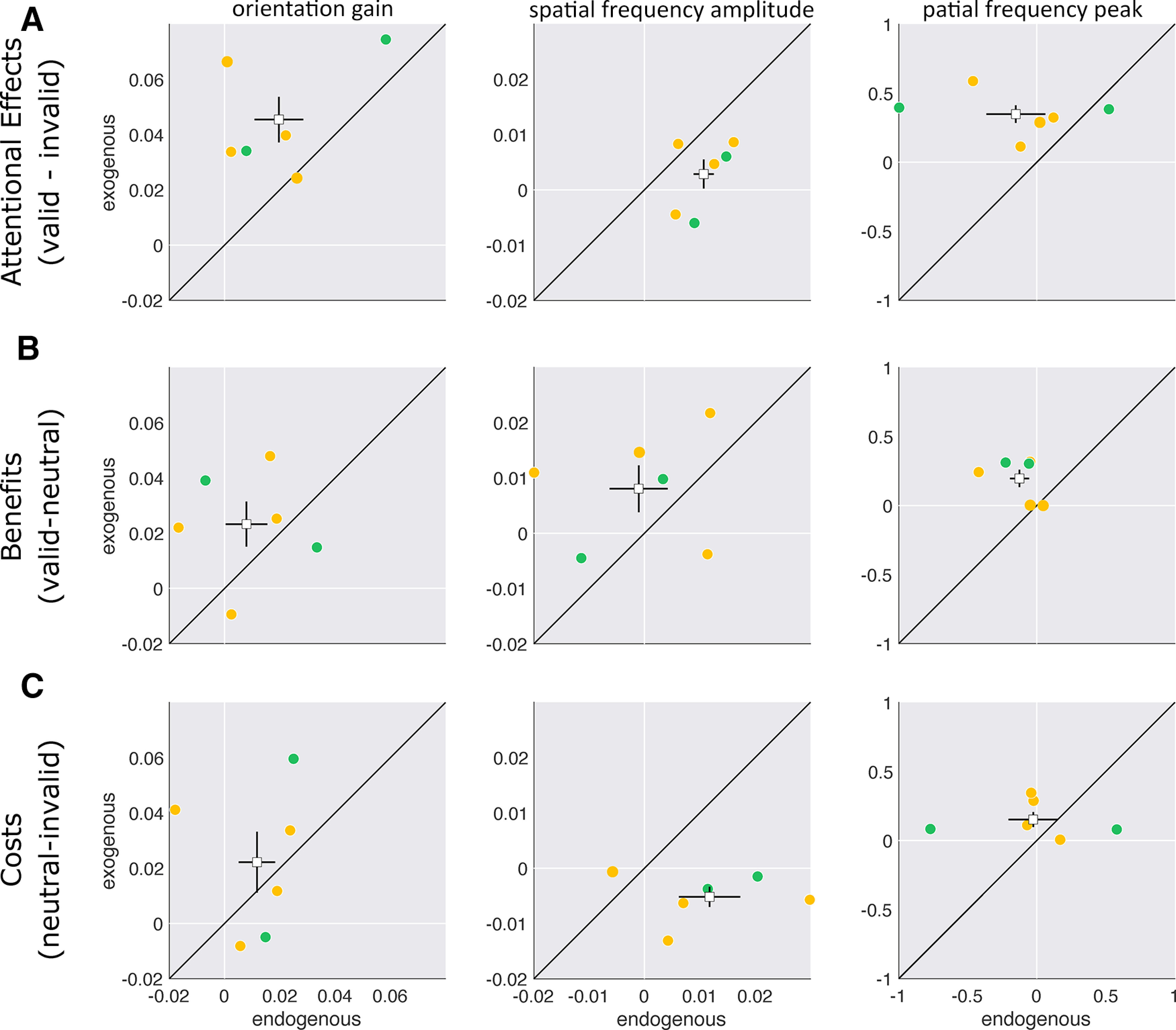
Attentional effects, benefits, and costs. A–C, Scatter plots of attentional effects (valid minus invalid; A), benefits (valid minus neutral; B), and costs (neutral minus invalid; C) for endogenous versus exogenous attention computed from fits to the individual data from parameter estimates for orientation gain, SF amplitude, and SF peak. orange circles are individual observers; green circles are author's data; white squares are group means. Error bars are ±1 SEM.

Computational modeling of behavioral effects

Based on a well established feedforward model of attention (Fig. 10A; see Materials and Methods), we successfully recovered each observer's performance in both experiment 1 (r = 0.98, p < 0.001) and experiment 2 (r = 0.97, p < 0.001; Fig. 10B). Additionally, when examining target-absent trials, the responses of the model displayed similar shifts to lower spatial frequencies with endogenous attention and to higher spatial frequencies with exogenous attention. With endogenous attention, the maximally responding spatial frequency channel was significantly lower with the valid than with the neutral and invalid cues (Fig. 10C; all p values < 0.001). The opposite was true with exogenous attention; the maximally responding spatial frequency channel was significantly higher with the valid than with the neutral and invalid cues (Fig. 10D; all p values < 0.001).

Figure 10.

Computational model. A, Model framework: consider that each pixel in the image labeled energy is a neuron; the excitatory drive of these neurons (numerator) is given by its input drive (stimulus energy) and attention. The suppressive drive (denominator) is given by the sum of the excitation across all neurons plus a constant. The maximally responding neuron after normalization is compared with a criterion, if the neuron response exceeds this criterion, the model says present; otherwise, it says absent. B, Mean observed versus predicted performance across 1000 bootstrapped iterations. C, D, Error bars indicate ±3 SEM SF preference for the maximally responding neuron across bootstrapped iterations for endogenous (C) and exogenous (D) attention. E, F, Model comparisons for endogenous (E) and exogenous (F) attention. Core: Core model where the kernel and stimulus energy are taken from the output of reverse correlation; random kernel, stimulus energy remains the same, but the kernel is a random noise image; random input, the kernel remains the same, but the stimulus energy is random.

To rule out that the responses of our model were merely driven either by the kernel (e.g., returning the attentional kernels as the output) or by the input drive (stimulus energy), we tested two other models for endogenous (Fig. 10E) and exogenous (Fig. 10F) attention: (1) the kernel is a random noise image across trials, but the input drive remains the same as the core model; and (2) the input drive is random noise but the kernels remain the same as the core model. The core model, containing the observer's kernels and stimulus energy, clearly outperformed the two competing models.

Discussion

We have compared the effects of endogenous and exogenous attention on orientation and SF tuning, with the same observers, tasks, and stimuli. Both types of attention yielded similar benefits in detection sensitivity at the attended location and costs at unattended locations, ruling out performance differences as a possible explanation for the differences in sensory tuning. In both experiments, reaction times were fastest for valid cues and slowest for invalid cues, ruling out speed–accuracy trade-offs, and there were no cue differences in decision criterion. These results, which are consistent with a normalization model of attention, provide critical evidence that endogenous and exogenous attention shape sensory representation in a distinct manner.

Orientation tuning

For both endogenous and exogenous attention, we found only gain changes, consistent with previous studies (Baldassi and Verghese, 2005; Paltoglou and Neri, 2012; Wyart et al., 2012; Barbot et al., 2014; Fernández et al., 2019). Comparing the magnitude of the overall attentional effects as well as of the benefits and costs revealed a stronger modulation by exogenous than endogenous attention. A possible explanation relates to the involuntary versus voluntary nature of the effect; exogenous attention exerts its effects automatically to the same degree regardless of cue validity, whereas the effect of endogenous attention increases with cue validity (Giordano et al., 2009). Although cue validity for endogenous was high (75%), the effects could have been more pronounced had the cue been 100% valid. This gain difference could also be related to attentional modulations of neural activity by exogenous attention being approximately constant from early visual areas (V1, V2, V3: Müller and Kleinschmidt, 2007; Müller and Ebeling, 2008; Dugué et al., 2020) to intermediate visual areas [V3A, hV4, LO1 (Dugué et al., 2020)], but increasing with endogenous attention from early to intermediate visual areas [Dugué et al., 2020; MT, VIP (ventral intraparietal; Maunsell and Cook, 2002)] to parietal and frontal areas (Kastner et al., 1999). Consistent with the idea that endogenous attention is a top-down modulation from frontal and parietal areas feeding back to visual cortex (for review, see Beck and Kastner, 2009; Chica et al., 2013). In any case, future research could assess whether this result is because of a mechanistic effect of attention or to the experimental parameters used here.

SF tuning

The SF data for both experiments was fit with the same model—shared parameter for the width. For endogenous attention, there was an overall increased amplitude of SFs above and below the target SF; this amplitude difference was primarily driven by the invalid cue. The overall amplitude difference is consistent with endogenous attention excluding external noise without changing SF tuning (Lu and Dosher, 2004). Additionally, peak sensitivity shifted to lower SFs than the neutral curve. Endogenous attention could have flexibly shifted sensitivity to lower SFs to counteract any effect of masking by the target SF (Meese and Hess, 2004). Exogenous attention shifted peak sensitivity to SFs higher than those for the neutral and invalid functions. This valid shift led to a preferential gain enhancement at SFs above the target SF.

Psychophysical studies using both reverse correlation (Fernández et al., 2019) and critical band masking (Talgar et al., 2004) had found no change in SF tuning with exogenous attention. Here, we capitalized on recent psychophysical findings to improve our task design. We hypothesize that the biggest contributors for the observed preferential enhancement of high SFs with exogenous attention were as follows: (1) placing stimuli at less eccentric locations; and (2) increasing the target SF. In our previous study (Fernández et al., 2019), the stimuli were placed at 10° eccentricity, and the target SF was 1.5 cpd, outside the optimal range of cueing benefits with exogenous attention (Jigo and Carrasco, 2020). By decreasing the eccentricity and increasing the target SF, we optimized stimulus parameters and could observe shifts in sensory tuning induced by exogenous attention.

A recent study has also revealed the differential effects of exogenous and endogenous attention on contrast sensitivity (indexed by $d\prime$; Jigo and Carrasco, 2020). Exogenous attention preferentially enhances SFs higher than the intrinsic peak frequency in a neutral baseline condition, whereas endogenous attention similarly benefits a broad range of SFs above and below the peak at baseline. Conventional signal detection theory is agnostic as to the underlying computation. Here, using reverse correlation, we show the computation (gain changes) that may underlie the differential effects of endogenous and exogenous attention and compare differences in gain modulation between both types of attention.

Psychophysical reverse correlation characterizes early sensory mechanisms and typically produces tuning curves akin to those derived from neural recordings (Neri and Levi, 2006). To link our behavioral measures to established neural computations, we incorporated the attentional kernels derived from reverse correlation into a normalization model of attention based on the study by Reynolds and Heeger (2009). The model captured each individual observer's performance in the task as well as the shifts in SF sensitivity, without imposing them (the model was unconstrained in the SF dimension). We reasoned that if the attentional kernels derived from reverse correlation are a true estimate of sensory weighting, then the reported shifts in peak SF should arise from a combination of the input drive and the attentional kernels. This was indeed the case.

Recently, a normalization model of attention has been developed to explain how endogenous and exogenous attention differentially alter visual perception (Jigo et al., 2021). To capture the effects of each of these types of attention on contrast sensitivity (Jigo and Carrasco, 2020), texture segmentation (Yeshurun and Carrasco, 1998; Barbot and Carrasco, 2017), and acuity (Montagna et al., 2009), the model requires the following SF tuning profiles consistent with the ones revealed in the present study: (1) a narrow high SF enhancement with exogenous attention; and (2) a broad SF profile with endogenous attention. Without differential SF profiles, the model cannot capture these established behavioral differences. Critically, these SF profiles scale the stimulus drive, suggesting that these differential effects between endogenous and exogenous attention arise at a sensory rather than at a decision stage, consistent with our modeling in the present study.

The present results are consistent with attentional gain, which is a well established computation occurring throughout many visual areas (for review, see Reynolds and Heeger, 2009; Bisley, 2011; Maunsell, 2015). For example, neural recordings from macaque areas V1, V2, V4, and MT have shown that covert spatial attention alters neural tuning via multiplicative gain (Motter, 1993; Treue and Martínez-Trujillo, 1999; Reynolds et al., 2000; Williford and Maunsell, 2006).

Our findings can inform neurophysiological research, given the similarities in spatial vision and attention between human and nonhuman primates. For example, sensitivity is higher for intermediate SFs (2–5 cpd) than for lower and higher SFs (humans: Campbell and Robson, 1968; nonhuman primates: Harwerth and Smith, 1985) and declines with increasing eccentricity (Sasaoka et al., 2005). Moreover, covert spatial attention improves contrast sensitivity and acuity in human (Montagna et al., 2009; Herrmann et al., 2010) and nonhuman (Golla et al., 2004; Pham et al., 2018) primates. Given the current findings, future neurophysiological studies focused on the modulatory effect on attention of sensory tuning and could assess whether gain modulations by endogenous attention would be similar for neurons coding SFs lower and higher than those of the target SF, whereas gain modulations by exogenous attention would preferentially enhance the gain of neurons tuned to higher SFs than the target SF.

What is the functional significance of the observed differences in SF tuning between endogenous and exogenous attention? When increasing resolution is not beneficial (e.g., driving through fog), the flexible, voluntarily controlled endogenous attention would be necessary. In fight-or-flight situations, an exogenous attentional system that is quick and reactive, and inflexibly increases resolution would be beneficial. Mice exhibit primate-like behavioral signatures of both endogenous and exogenous attention (You and Mysore, 2020) despite having poorer contrast sensitivity (Histed et al., 2012) and no fovea. Additionally, mice show increased gain in neurons tuned for high SFs under a state of heightened attention, thereby increasing their spatial acuity (Mineault et al., 2016). Despite pronounced differences in the visual system of mice and primates, a similar mechanism (e.g., attention) may underlie sensory tuning properties in mammals. Therefore, understanding how attention reshapes the sensory tuning of basic visual dimensions is of critical importance. Furthermore, our findings help constrain models of spatial vision and of visual attention by furthering our knowledge of the neural computations underlying the effects of covert spatial attention on basic dimensions of spatial vision and provide further empirical evidence for the differential SF profiles required to model the distinct effects of endogenous and exogenous attention on perception (Jigo et al., 2021).

To conclude, this study reveals the differential effects of endogenous and exogenous attention on sensory tuning. Both types of covert attention modulate orientation at the attended location by boosting the gain of all orientation channels without changing tuning width. This boost was greater with exogenous than endogenous attention. In the SF domain, endogenous attention enhanced the gain of SFs above and below the target SF, whereas exogenous attention only enhanced those above. We propose that these changes in sensory tuning may underlie the differential effects of endogenous and exogenous attention on performance.

References

- Acerbi L, Ma WJ (2017) Practical Bayesian optimization for model fitting with Bayesian adaptive direct search. In: NIPS 2017 31st annual conference on neural information processing systems (von Luxburg R, Guyon R, Bengio R, Wallach H, Fergus R, Vishwanathan SVN, Garnett R, eds), pp 1834–1844. Red Hook, NY: Curran Associates. [Google Scholar]
- Ahumada AJ Jr (1996) Perceptual classification images from Vernier acuity masked by noise. Perception 25 [suppl]:2-2. 10.1068/v96l0501 [DOI] [Google Scholar]
- Anton-Erxleben K, Carrasco M (2013) Attentional enhancement of spatial resolution: linking behavioural and neurophysiological evidence. Nat Rev Neurosci 14:188–200. [DOI] [PMC free article] [PubMed] [Google Scholar]
- Bakeman R (2005) Recommended effect size statistics for repeated measures designs. Behav Res Methods 37:379–384. 10.3758/bf03192707 [DOI] [PubMed] [Google Scholar]
- Baldassi S, Verghese P (2005) Attention to locations and features: different top-down modulation of detector weights. J Vis 5:556–570. 10.1167/5.6.7 [DOI] [PubMed] [Google Scholar]
- Barbot A, Carrasco M (2017) Attention modifies spatial resolution according to task demands. Psychol Sci 28:285–296. [DOI] [PMC free article] [PubMed] [Google Scholar]
- Barbot A, Wyart V, Carrasco M (2014) Spatial and feature-based attention differentially affect the gain and tuning of orientation-selective filters. J Vis 14:703. 10.1167/14.10.703 [DOI] [Google Scholar]
- Beck DM, Kastner S (2009) Top-down and bottom-up mechanisms in biasing competition in the human brain. Vision Res 49:1154–1165. [DOI] [PMC free article] [PubMed] [Google Scholar]
- Bisley JW (2011) The neural basis of visual attention. J Physiol 589:49–57. 10.1113/jphysiol.2010.192666 [DOI] [PMC free article] [PubMed] [Google Scholar]
- Bloem IM, Ling S (2019) Normalization governs attentional modulation within human visual cortex. Nat Commun 10:1–10. 10.1038/s41467-019-13597-1 [DOI] [PMC free article] [PubMed] [Google Scholar]
- Brainard DH (1997) The psychophysics toolbox. Spat Vis 10:433–436. 10.1163/156856897X00357 [DOI] [PubMed] [Google Scholar]
- Burnham KP, Anderson DR (2002) Model selection and multimodel inference: a practical information-theoretic approach, Ed 2. New York: Springer. [Google Scholar]
- Busse L, Katzner S, Treue S (2008) Temporal dynamics of neuronal modulation during exogenous and endogenous shifts of visual attention in macaque area MT. Proc Natl Acad Sci U S A 105:16380–16385. 10.1073/pnas.0707369105 [DOI] [PMC free article] [PubMed] [Google Scholar]
- Campbell FW, Robson JG (1968) Application of Fourier analysis to the visibility of gratings. The Journal of physiology 197:551–566. [DOI] [PMC free article] [PubMed] [Google Scholar]
- Carandini M, Heeger DJ (2012) Normalization as a canonical neural computation. Nat Rev Neurosci 13:51–62. 10.1038/nrn3136 [DOI] [PMC free article] [PubMed] [Google Scholar]
- Carrasco M (2011) Visual attention: the past 25 years. Vision Res 51:1484–1525. 10.1016/j.visres.2011.04.012 [DOI] [PMC free article] [PubMed] [Google Scholar]
- Carrasco M (2014) Spatial covert attention: perceptual modulation. In: The Oxford handbook of attention (Nobre K, Kastner S, eds), pp 183–230. Oxford, UK: Oxford UP. [Google Scholar]
- Carrasco M, Barbot A (2014) How attention affects spatial resolution. Cold Spring Harb Symp Quant Biol 79:149–160. 10.1101/sqb.2014.79.024687 [DOI] [PMC free article] [PubMed] [Google Scholar]
- Carrasco M, Loula F, Ho YX (2006) How attention enhances spatial resolution: evidence from selective adaptation to spatial frequency. Percept Psychophys 68:1004–1012. [DOI] [PubMed] [Google Scholar]
- Chica AB, Bartolomeo P, Lupiáñez J (2013) Two cognitive and neural systems for endogenous and exogenous spatial attention. Behav Brain Res 237:107–123. [DOI] [PubMed] [Google Scholar]
- Cohen J (1992) A power primer. Psychol Bull 112:155–159. 10.1037/0033-2909.112.1.155 [DOI] [PubMed] [Google Scholar]
- Dugué L, Merriam EP, Heeger DJ, Carrasco M (2020) Differential impact of endogenous and exogenous attention on activity in human visual cortex. Sci Rep 10:1–16. 10.1038/s41598-020-78172-x [DOI] [PMC free article] [PubMed] [Google Scholar]
- Eckstein MP, Ahumada AJ (2002) Classification images: a tool to analyze visual strategies. J Vis 2:1x. 10.1167/2.1.i [DOI] [PubMed] [Google Scholar]
- Fernández A, Carrasco M (2020) Extinguishing exogenous attention via transcranial magnetic stimulation. Curr Biol 30:4078–4084. [DOI] [PMC free article] [PubMed] [Google Scholar]
- Fernández A, Li HH, Carrasco M (2019) How exogenous spatial attention affects visual representation. J Vis 19(11):4, 1–13. 10.1167/19.11.4 [DOI] [PMC free article] [PubMed] [Google Scholar]
- Giordano AM, McElree B, Carrasco M (2009) On the automaticity and flexibility of covert attention: a speed-accuracy trade-off analysis. J Vis 9(3):30, 1–10. 10.1167/9.3.30 [DOI] [PMC free article] [PubMed] [Google Scholar]
- Golla H, Ignashchenkova A, Haarmeier T, Thier P (2004) Improvement of visual acuity by spatial cueing: a comparative study in human and non-human primates. Vision Res 44:1589–1600. [DOI] [PubMed] [Google Scholar]
- Harwerth RS, Smith EL (1985) Rhesus monkey as a model for normal vision of humans. Am J Optom Physiol Opt 62:633–641. [DOI] [PubMed] [Google Scholar]
- Herrmann K, Montaser-Kouhsari L, Carrasco M, Heeger DJ (2010) When size matters: attention affects performance by contrast or response gain. Nat Neurosci 13:1554–1559. 10.1038/nn.2669 [DOI] [PMC free article] [PubMed] [Google Scholar]
- Herrmann K, Heeger DJ, Carrasco M (2012) Feature-based attention enhances performance by increasing response gain. Vision Res 74:10–20. [DOI] [PMC free article] [PubMed] [Google Scholar]
- Histed MH, Carvalho LA, Maunsell JH (2012) Psychophysical measurement of contrast sensitivity in the behaving mouse. J Neurophysiol 107:758–765. [DOI] [PMC free article] [PubMed] [Google Scholar]
- Holm S (1979) A simple sequentially rejective multiple test procedure. Scand J Stat 6:65–70. [Google Scholar]
- Hubel DH, Wiesel TN (1959) Receptive fields of single neurons in the cat's striate cortex. J of Physiol 148:574–591. 10.1113/jphysiol.1959.sp006308 [DOI] [PMC free article] [PubMed] [Google Scholar]
- Jigo M, Carrasco M (2018) Attention alters spatial resolution by modulating second-order processing. J Vis 18(7):2, 1–12. [DOI] [PMC free article] [PubMed] [Google Scholar]
- Jigo M, Carrasco M (2020) Differential impact of exogenous and endogenous attention on the contrast sensitivity function across eccentricity. J Vis 20(6):11, 1–25. [DOI] [PMC free article] [PubMed] [Google Scholar]
- Jigo M, Heeger DJ, Carrasco M (2021) An image-computable model on how endogenous and exogenous attention differentially alter visual perception. Proc Natl Acad Sci U S A 118:e2106436118. 10.1073/pnas.2106436118 [DOI] [PMC free article] [PubMed] [Google Scholar]
- Kastner S, Pinsk MA, De Weerd P, Desimone R, Ungerleider LG (1999) Increased activity in human visual cortex during directed attention in the absence of visual stimulation. Neuron 22:751–761. [DOI] [PubMed] [Google Scholar]
- Kleiner M, Brainard D, Pelli D, Ingling A, Murray R, Broussard C (2007) What's new in Psychtoolbox-3. Perception 36:1–16. [Google Scholar]
- Lennie P (2003) The cost of cortical computation. Current biology 13:493–497. [DOI] [PubMed] [Google Scholar]
- Li HH, Barbot A, Carrasco M (2016) Saccade preparation reshapes sensory tuning. Curr Biol 26:1564–1570. [DOI] [PMC free article] [PubMed] [Google Scholar]
- Li HH, Pan J, Carrasco M (2019) Presaccadic attention improves or impairs performance by enhancing sensitivity to higher spatial frequencies. Sci Rep 9:2659. 10.1038/s41598-018-38262-3 [DOI] [PMC free article] [PubMed] [Google Scholar]
- Li HH, Pan J, Carrasco M (2021) Different computations underlie overt presaccadic and covert spatial attention. Nat Hum Behav 1–14. [DOI] [PMC free article] [PubMed] [Google Scholar]
- Ling S, Carrasco M (2006) Sustained and transient covert attention enhance the signal via different contrast response functions. Vision Res 46:1210–1220. [DOI] [PMC free article] [PubMed] [Google Scholar]
- Lu ZL, Dosher BA (2004) Spatial attention excludes external noise without changing the spatial frequency tuning of the perceptual template. J Vis 4:955–966. 10.1167/4.10.10 [DOI] [PubMed] [Google Scholar]
- Macmillan NA, Creelman CD (2004) Detection theory: a user's guide. Abingdon-on-Thames, UK: Psychology Press. [Google Scholar]
- Maffei L, Fiorentini A (1977) Spatial frequency rows in the striate visual cortex. Vision Res 17:257–264. 10.1016/0042-6989(77)90089-X [DOI] [PubMed] [Google Scholar]
- Masson ME (2011) A tutorial on a practical Bayesian alternative to null-hypothesis significance testing. Behav Res Methods 43:679–690. 10.3758/s13428-010-0049-5 [DOI] [PubMed] [Google Scholar]
- Maunsell JH (2015) Neuronal mechanisms of visual attention. Annual Review of Vision Science 1:373–391. [DOI] [PMC free article] [PubMed] [Google Scholar]
- Maunsell JH, Cook EP (2002) The role of attention in visual processing. Philos Trans R Soc Lond B Biol Sci 357:1063–1072. 10.1098/rstb.2002.1107 [DOI] [PMC free article] [PubMed] [Google Scholar]
- Meese TS, Hess RF (2004) Low spatial frequencies are suppressively masked across spatial scale, orientation, field position, and eye of origin. J Vis 4:843–859. 10.1167/4.10.2 [DOI] [PubMed] [Google Scholar]
- Mineault PJ, Tring E, Trachtenberg JT, Ringach DL (2016) Enhanced spatial resolution during locomotion and heightened attention in mouse primary visual cortex. J Neurosci 36:6382–6392. 10.1523/JNEUROSCI.0430-16.2016 [DOI] [PMC free article] [PubMed] [Google Scholar]
- Montagna B, Pestilli F, Carrasco M (2009) Attention trades off spatial acuity. Vision Res 49:735–745. [DOI] [PMC free article] [PubMed] [Google Scholar]
- Morrone MC, Denti V, Spinelli D (2002) Color and luminance contrasts attract independent attention. Curr Biol 12:1134–1137. 10.1016/S0960-9822(02)00921-1 [DOI] [PubMed] [Google Scholar]
- Morrone MC, Denti V, Spinelli D (2004) Different attentional resources modulate the gain mechanisms for color and luminance contrast. Vision Res 44:1389–1401. [DOI] [PubMed] [Google Scholar]
- Motter BC (1993) Focal attention produces spatially selective processing in visual cortical areas V1, V2, and V4 in the presence of competing stimuli. J Neurophysiol 70:909–919. 10.1152/jn.1993.70.3.909 [DOI] [PubMed] [Google Scholar]
- Müller NG, Ebeling D (2008) Attention-modulated activity in visual cortex—more than a simple “spotlight”. Neuroimage 40:818–827. [DOI] [PubMed] [Google Scholar]
- Müller NG, Kleinschmidt A (2007) Temporal dynamics of the attentional spotlight: neuronal correlates of attentional capture and inhibition of return in early visual cortex. J Cogn Neurosci 19:587–593. 10.1162/jocn.2007.19.4.587 [DOI] [PubMed] [Google Scholar]
- Neri P, Levi DM (2006) Receptive versus perceptive fields from the reverse-correlation viewpoint. Vision Res 46:2465–2474. [DOI] [PubMed] [Google Scholar]
- Ni AM, Maunsell JH (2017) Spatially tuned normalization explains attention modulation variance within neurons. J Neurophysiol 118:1903–1913. 10.1152/jn.00218.2017 [DOI] [PMC free article] [PubMed] [Google Scholar]
- Ni AM, Maunsell JH (2019) Neuronal effects of spatial and feature attention differ due to normalization. J Neurosci 39:5493–5505. [DOI] [PMC free article] [PubMed] [Google Scholar]
- Paltoglou AE, Neri P (2012) Attentional control of sensory tuning in human visual perception. J Neurophysiol 107:1260–1274. [DOI] [PMC free article] [PubMed] [Google Scholar]
- Pelli DG (1997) The VideoToolbox software for visual psychophysics: transforming numbers into movies. Spat Vis 10:437–442. 10.1163/156856897X00366 [DOI] [PubMed] [Google Scholar]
- Pentland A (1980) Maximum likelihood estimation: the best PEST. Percept Psychophys 28:377–379. 10.3758/bf03204398 [DOI] [PubMed] [Google Scholar]
- Pestilli F, Ling S, Carrasco M (2009) A population-coding model of attention's influence on contrast response: estimating neural effects from psychophysical data. Vision Res 49:1144–1153. [DOI] [PMC free article] [PubMed] [Google Scholar]
- Pham A, Carrasco M, Kiorpes L (2018) Endogenous attention improves perception in amblyopic macaques. J Vis 18(3):11, 1–13. [DOI] [PMC free article] [PubMed] [Google Scholar]
- Reynolds JH, Heeger DJ (2009) The normalization model of attention. Neuron 61:168–185. [DOI] [PMC free article] [PubMed] [Google Scholar]
- Reynolds JH, Pasternak T, Desimone R (2000) Attention increases sensitivity of V4 neurons. Neuron 26:703–714. [DOI] [PubMed] [Google Scholar]
- Rolke B, Dinkelbach A, Hein E, Ulrich R (2008) Does attention impair temporal discrimination? Examining non-attentional accounts. Psychol Res 72:49–60. [DOI] [PubMed] [Google Scholar]
- Sasaoka M, Hara H, Nakamura K (2005) Comparison between monkey and human visual fields using a personal computer system. Behav Brain Res 161:18–30. [DOI] [PubMed] [Google Scholar]
- Sharp P, Melcher D, Hickey C (2018) Endogenous attention modulates the temporal window of integration. Atten Percept Psychophys 80:1214–1228. 10.3758/s13414-018-1506-y [DOI] [PubMed] [Google Scholar]
- Talgar CP, Carrasco M (2002) Vertical meridian asymmetry in spatial resolution: visual and attentional factors. Psychon Bull Rev 9:714–722. 10.3758/bf03196326 [DOI] [PubMed] [Google Scholar]
- Talgar CP, Pelli DG, Carrasco M (2004) Covert attention enhances letter identification without affecting channel tuning. J Vis 4:22–31. 10.1167/4.1.3 [DOI] [PubMed] [Google Scholar]
- Treue S, Martínez-Trujillo JC (1999) Feature-based attention influences motion processing gain in macaque visual cortex. Nature 399:575–579. 10.1038/21176 [DOI] [PubMed] [Google Scholar]
- Watson AB, Ahumada AJ (2005) A standard model for foveal detection of spatial contrast. J Vis. 5:6–6. 10.1167/5.9.6 [DOI] [PubMed] [Google Scholar]
- Wichmann FA, Hill NJ (2001) The psychometric function: I. Fitting, sampling, and goodness of fit. Perception & psychophysics 63:1293–1313. [DOI] [PubMed] [Google Scholar]
- Williford T, Maunsell JH (2006) Effects of spatial attention on contrast response functions in macaque area V4. J Neurophysiol 96:40–54. [DOI] [PubMed] [Google Scholar]
- Wyart V, Nobre AC, Summerfield C (2012) Dissociable prior influences of signal probability and relevance on visual contrast sensitivity. Proc Natl Acad Sci U S A 109:3593–3598. 10.1073/pnas.1120118109 [DOI] [PMC free article] [PubMed] [Google Scholar]
- Yeshurun Y (2004) Isoluminant stimuli and red background attenuate the effects of transient spatial attention on temporal resolution. Vision Res 44:1375–1387. 10.1016/j.visres.2003.12.016 [DOI] [PubMed] [Google Scholar]
- Yeshurun Y, Carrasco M (1998) Attention improves or impairs visual performance by enhancing spatial resolution. Nature 396:72–75. 10.1038/23936 [DOI] [PMC free article] [PubMed] [Google Scholar]
- Yeshurun Y, Carrasco M (2000) The locus of attentional effects in texture segmentation. Nat Neurosci 3:622–627. [DOI] [PubMed] [Google Scholar]
- Yeshurun Y, Hein E (2011) Transient attention degrades perceived apparent motion. Perception 40:905–918. [DOI] [PubMed] [Google Scholar]
- Yeshurun Y, Levy L (2003) Transient spatial attention degrades temporal resolution. Psychol Sci 14:225–231. 10.1111/1467-9280.02436 [DOI] [PubMed] [Google Scholar]
- Yeshurun Y, Montagna B, Carrasco M (2008) On the flexibility of sustained attention and its effects on a texture segmentation task. Vision Res 48:80–95. [DOI] [PMC free article] [PubMed] [Google Scholar]
- You WK, Mysore SP (2020) Endogenous and exogenous control of visuospatial selective attention in freely behaving mice. Nat Commun 11:1–14. 10.1038/s41467-020-15909-2 [DOI] [PMC free article] [PubMed] [Google Scholar]