Cactus Graphs for Genome Comparisons

Abstract

We introduce a data structure, analysis, and visualization scheme called a cactus graph for comparing sets of related genomes. In common with multi-break point graphs and A-Bruijn graphs, cactus graphs can represent duplications and general genomic rearrangements, but additionally, they naturally decompose the common substructures in a set of related genomes into a hierarchy of chains that can be visualized as two-dimensional multiple alignments and nets that can be visualized in circular genome plots. Supplementary Material is available at www.liebertonline.com/cmb.

1. Introduction

Genomes are compared by forming alignments in which the bases are grouped into sets that share common ancestry, commonly termed homology. At a fine scale, genomes can often be assumed to differ only by rearrangements that substitute, insert, and delete bases. Such alignments are typically represented as two-dimensional matrices in which the rows represent the sequences interspersed with gaps, and the columns represent groups of homologous bases (Higgins et al., 1992). More recently these alignments have also been represented as directed acyclic graphs (DAGs) within which the sequences are encoded (Lee et al., 2002), the advantage being that the groupings of homologous bases need only be partially ordered, for example, when there is genuine uncertainty about the ordering of two neighboring insertions or deletions.

At a large scale, genomes are subject to rearrangements that prevent them from being represented in either a matrix or a DAG. For pairs of genomes, large-scale alignments are typically represented as break point graphs (Hannenhalli and Pevzner, 1995); for large scale multiple genome comparison, either multi-break point graphs (Alekseyev and Pevzner, 2008) or A-Bruijn graphs are used (Pevzner et al., 2004). The differences between the representations of large-scale and fine-scale analysis have led to divergent sets of algorithms and methods for analysis. This dichotomy between the largest and finest scales is of course false; the changes between genomes exhibit structure at many intermediate levels as well, but have largely arisen out computational necessity. The methods used for aligning at a fine scale, typically based upon dynamic programming with graphical models, such as hidden Markov models (Durbin et al., 1998), cannot be applied at the large scale because of non-linear rearrangements. Conversely, while efficient polynomial methods for reasoning about the distance, in terms of various classes of rearrangements, between two genomes represented in a breakpoint graph are well known (Hannenhalli and Pevzner, 1995, 1999; Yancopoulos et al., 2005)—many of the same problems become NP-hard for three or more genomes (Caprara, 1999; Tannier et al., 2009)—methods for forming a large-scale homology map are still in their relative infancy, with little agreement even about what objective function to optimize (Raphael et al., 2004; Brudno et al., 2003).

Previously, Bergeron and Stoye (2006) and Bergeron et al. (2004) showed how, in the study of rearrangements between sets of genomes, the structure of genome change is inherently nested, with small rearrangements inside of larger rearrangements. In their work, which is also strongly related to the notion of the overlap graph in the sorting by reversals and translocations problem (Hannenhalli and Pevzner, 1995) and the sorting by reversals problem (Hannenhalli and Pevzner, 1999), they defined the notion of conserved intervals within sets of signed permutations, and showed that these conserved intervals could both be nested and organised into sequences. Such organizing structure is desirable, because it gives rise to data structures to represent genome comparisons that have explicit tree-like substructure, allowing for both more efficient storage and computation. In this work, we introduce a data structure to genome comparison called a cactus graph (Harary and Uhlenbeck, 1953) that generalizes the notion of conserved intervals and their hierarchies, allowing for multiple sequences and arbitrary duplication, such that two or more elements from one genome may be considered homologous. The abstract combinatorial notion of a cactus graph has also been used in many different optimization problems, including graph decomposition (Korneyenko, 1994), optimal traffic (Zamazek and Zerovnik, 2005) and facility location problems (Ben-Moshe and Bhattacharya, 2005), and electrical circuits (Tetsuo, 1991).

In the next section, we describe in overview the proposed cactus graph data structure. For the reader uninterested in the methodological details, this section should be sufficient to understand the essentials of the idea. For readers wishing to read the remainder of the article, this section is necessary as it defines essential terminology.

2. Overview

The first step in genome comparison is to identify and align segments of DNA that are homologous between and within the genomes being compared. These segments may be, for example, coding exons, recognizably conserved noncoding elements, or large orthologous chromosomal regions of closely related genomes. A two-dimensional multiple alignment (as described above) of a set of homologous segments differing only by base substitutions is called a block.

Identification of the segments leaves behind stretches of unaligned DNA that we call adjacencies between segments and at the ends of chromosomes. To make the two adjacencies at the opposite ends of a chromosome into proper adjacencies, we add a cap at each end representing the telomeres, and connect these two caps by adjacencies to the first and last segments. More generally, a cap can be the end of any sequence of DNA. Thus, when applying these conventions to represent an internal part of a chromosome, the caps are the ends of the segments flanking this internal part of the chromosome. We define a thread as a path of alternating adjacencies and segments connected by caps that is flanked by adjacencies connected to caps.

Caps naturally inherit the homologies of the segment ends that define them. Additional homologies can be defined a priori for chromosome telomeres, so that all caps, be they internal segment ends or chromosome telomeres, are treated in the same fashion. A family of homologous caps is called an end.

A net is a graph in which each node is an end and each edge represents a set of adjacencies between the caps in the two ends it connects. A complete net for the comparison of a set of genomes has a node for each end of every block and a node for each telomere end. There is an edge between two nodes whenever there is an adjacency between them in any of the genomes being compared. Usually, the nodes are laid out on a circle, and the edges are geodesics that cross the circle (Fig. 1) (Carver et al., 2009; Krzywinski et al., 2009). Complete nets quickly get very dense and hard to interpret with growing genome size and genome distance; however, they can often be decomposed into smaller components. The cactus graph provides an organizing principle in which simpler subnets and nested substructures can be extracted from complete nets. For example, the four ends highlighted by curly braces in Figure 1 form a connected component of adjacencies for which we can construct a net as shown in Figure 2. In the “blue” genome, they appear as A₂ B A₃, and in the “green” genome they appear as A₂ −B A₃, where the negative sign denotes reverse complement. This inversion is represented cleanly in a simple subnet, separable from the larger complete net.

FIG. 1.

A circular genome style plot showing a complete net with examples of chains and threads. Blue and green lines depict two homologous threads traversing a series of segments in blocks and the joining adjacencies. All aligned boxes are blocks except A₁ and A₄, which are ends representing telomeres. The ends of the blocks and the ends of the telomeres are mapped as filled black rectangles on the edges of the aligned boxes. These are the nodes in the complete net. DNA bases within the adjacencies are not shown. Ignoring the unseen sequence within the adjacencies and starting at A₁, the blue thread gives the sequence ACTTGGCCACTGGGACGCCATCGGAAGTTCCagtGGGACGCCATCATCGGATCGACTGTTTCATGGATCCC. The green thread gives the sequence ACTGAAGACCGGATCGcatggccagtGAGC. The lower case “agt” in the blue thread represents the reverse complement of the bottom segment of block G₁, which is traversed right-to-left in the blue thread, and similarly, the lower case segment in the green thread is the reverse complement of segments in B₂, K₁ and B₁, also traversed right-to-left. Chains containing more than one block/end are given distinct colors; for example, chain A has two blocks, A₂ and A₃, and two ends, A₁ and A₄ in it, all colored red. The large curly brackets highlight the four ends of the subnet shown in Figure 2.

FIG. 2.

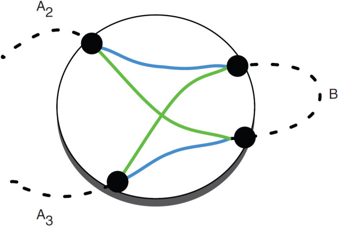
A net for the ends highlighted by curly brackets in Figure 1. The net is composed of four ends: an end of A₂, an end of A₃, an end of B₁, and an end of B₂, where B₁ and B₂ form a chain B. The ends are represented by the four filled circles on the larger circle. The adjacencies between the ends of the elements are the colored green and blue lines, the coloring indicating the two respective threads of Figure 1.

Each node of the cactus graph is a subnet of a complete net (see Section 4.1), as determined by the construction in Section 3.3, and each edge is a block. Every block in the genomes being compared appears as an edge, and every adjacency between segments or from a segment to a telomere cap is represented in one of the subnets. A simple cycle is a closed (simple) path, with no other repeated vertices or edges other than the starting and ending vertices. The cactus graph consists of a single connected component that is composed of a set of simple cycles, i.e., cycles such that no node is used twice, such that any two simple cycles intersect at at most one node (Fig. 3). This property gives it its “cactus-like” appearance. Each simple cycle in the graph has an orientation that determines the direction of each edge on the cycle (see Section 4.2). All the telomere ends are contained in a single subnet represented by a node called the origin. A hierarchical set of chains is defined as follows. For each simple cycle that includes the origin, we define a child chain by concatenating the blocks represented by the edges of the cycle in the order that they appear, starting from the first outgoing edge from the origin. Each node along this cycle, apart from the origin, represents a link in the chain. Conceptually, the link consists of that node and the entire sub-cactus graph that is attached to the chain at that node, i.e., the smaller cactus you would get if you pruned off this piece and replanted it. The origin node is called the parent of the child chain. Traversing outwardly from child chains of the origin node, the definition of further chains proceeds recursively. Each node in one of the previously found simple cycles for which we have not yet defined a chain set becomes a new origin-like node, and we define child chains for it in the manner above, until all nodes have been explored and all chains are children with unique parents. This recursion results in a hierarchical structure called the cactus tree, a bi-layered tree consisting of parent subnets describing the relative order and orientation of their child chains, and these chains in turn containing a subnet in each of their links that describes further chains nested inside these links, and so on (Fig. 4). This hierarchy represents the organization of the substructures shared between the genomes at various levels, from large chromosomal regions down to individual bases.

FIG. 3.

A cactus graph with embedded net substructures for the chains and threads in Figure 1. The blue and green lines again depict the two threads. Each net node is shown in a circle; the origin net is ϕ. Block and end edges are depicted with multiple arrows, representing the different threads traversing them. The dotted arrows of A₁ and A₄ indicate that they are stub ends. The lines within the circles represent the adjacencies. The dotted lines in net ϕ represent the backdoor adjacencies connecting the dead ends of A₁ and A₄.

FIG. 4.

A cactus tree for the cactus in Figure 3. Nets are shown as circles, chains as squares. The tree is bi-layered, with alternating net and chain layers.

In this manner, a cactus graph partitions a set of genomes into nested structures represented by chains and subnets analogous to those introduced in (Kent et al. (2003), which can be visualized using alignments and circular plots, respectively. As an example, let us suppose that we are comparing a set of genomes in which only the coding exons are aligned, and these genomes include some genes within the introns of other genes, which may be duplicated or inverted in some cases, as can be the enclosing genes. In this case, there will be a block for every set of homologous exons, and there will be a top-level chain in the cactus tree for the exons of every top-level gene or subsequence of genes that remain in the same order and orientation in all the genomes being compared. Nested inside of these chains will be further chains for top-level genes whose order is rearranged between the genome (e.g., by inversion in a subset of the genomes). At deeper levels still, there will be chains for genes that appear in the introns of enclosing genes and vary between genomes.

3. Cactus Graphs

In this section, we formally describe the construction of the cactus graph.

3.1. Basepairs and chromosomes

Let S be the set of input chromosomes. Here we assume the input chromosomes are either linear or circular sequences; in Section 5, we consider the construction stages with missing data. Mathematically, a chromosome is just a string, possibly circular, of signed symbols taken from a fixed alphabet of possible symbols. There are only two unoriented basepairs, A/T and G/C, but we distinguish A/T from its reverse orientation T/A, termed its reverse complement, and similarly G/C from its reverse complement C/G, using signs we hence can equivalently write −A/T = T/A, −T/A = A/T, −G/C = C/G, and −G/C = C/G. The alphabet is therefore the oriented symbols {A/T, T/A, C/G, and G/C}. Each circular chromosome added to S is broken at an arbitrary adjacency, which we call the backdoor adjacency; thus, for the remainder of the construction, circular chromosomes can be treated as linear chromosomes with an extra piece of information recording that their two ends are actually contiguous.

3.2. Homology

We say that two oriented basepairs in S are homologous, denoted x ∼ y, if they are related to each other by some given biological definition of relatedness, e.g., if they descend from a common ancestral basepair that existed at a certain time in the past. As the homology relation is on the set of oriented base pairs in the sequences of S, if x ∼ y then −x ∼ −y but not x ∼ −y or −x ∼ y. For the purposes of this article, we require only that the notion of homology between oriented basepairs be an equivalence relation, i.e., is reflexive (x ∼ x), symmetric (if x ∼ y then y ∼ x), and transitive (if x ∼ y and y ∼ z then x ∼ z). Such an equivalence relation partitions the basepairs of S into equivalence classes, such that any two bases in the same equivalence class are related (homologous), but no two basepairs in different equivalence classes are related. Two oriented strings and are homologous if their bases are homologous, i.e., x ∼ y if x₁ ∼ y₁, , and x_n ∼ y_n.

3.3. Blocks, ends, adjacency graphs, and cactus graphs

The goal is to represent the common structure between substrings of homologous bases in S. To do this, we model two types of aforementioned homology structure: blocks and ends. A block is formally a maximal set of maximal-length homologous oriented strings. Each maximal length oriented string in a block is a segment. The blocks are shown as boxes containing gapless two-dimensional alignments in Figure 1, and the segments are shown as the rows of these alignments. Ends are maximal sets of homologous caps. We define two types of end for our graphs, block ends, which are the ends of blocks and stub ends, which include the previously mentioned telomeres, and which will also include block ends from higher level problems when we define multi-level cactus graphs (see Section 6).

The adjacency graph (Fig. 5 A) is a graph with a node for every end and an adjacency edge between two ends if there is an adjacency, potentially containing a nonempty substring from the input sequence, between a cap in one of the ends and a cap in the other end, i.e., if the caps would abut except for a possibly non-empty intervening adjacency substring in the input chromosome in which they appear. Self-edges are allowed in the adjacency graph and occur when two homologous caps in opposite orientation share an adjacency. Multi-edges are not included in the adjacency graph; i.e., there is at most one adjacency edge between any two nodes, even if there are several adjacencies between them. In this case, the adjacency edge is labeled with the set of adjacencies and their substrings, which uniquely pair caps between the ends they link. Unlike blocks, the substrings within the adjacencies of an adjacency edge are not assumed to be homologous and are therefore not aligned. The two ends of each block are also connected by an edge in the adjacency graph; these edges are called block edges and are labeled with the oriented set of aligned segments of the block they represent. In addition to the block edges, the adjacency graph also includes end edges; for each stub end, the adjacency graph includes one end edge that connects the node representing the stub end to a special dead-end node. All dead end nodes are in turn connected in a clique by unlabeled backdoor adjacency edges.

FIG. 5.

Examples graphs in the stages of construction of the final cactus graph from an initial adjacency graph. (A) G₀, an example adjacency graph. All black edges represent blocks except the black edges A and G, which are end edges; adjacency edges are gray, a backdoor adjacency (dotted gray edge) attaches the dead end nodes to one another. (B) G₁, the same graph after the collapse of the adjacency components. (C) G₂, after the collapse of the three-edge connected components. (D) G₃, after modifications to bridge edge components to make the graph Eulerian.

Let G₀ be the adjacency graph. The cactus graph is built from G₀ in a series of steps (Fig. 5).

1. (1) Ignoring the block and end edges, we compute the connected components of G₀ formed by the adjacency edges only. These are called adjacency-connected components. All dead ends will be in a single component, which we call the origin component. The graph G₁ represents this decomposition of G₀ into the resulting adjacency-connected components (Fig. 5B). There is a node in G₁ for every adjacency-connected component in G₀. The graph G₁ has only block and end edges, no adjacency edges. Two nodes X and Y in G₁,—representing (not necessarily distinct) adjacency-connected components in G₀—are connected by an edge in G₁ for every block or end edge in G₀ from some to some . Thus, the graph G₁ is formed by merging adjacency-connected nodes in G₀ and retaining only the block and end edges in the merged graph. We call the node in G₁ and subsequent graphs containing the origin component of G₀ the origin node.

2. (2) We compute the decomposition of G₁ into three-edge connected components using the linear time algorithm in Tsin (2007). To define this decomposition, we say that two nodes x and y in G₁ are equivalent if there is no set of up to two edges in G₁ which, upon removal, disconnect G₁ in such a way that there is no path from x to y. Thus, two nodes are equivalent if it takes the removal of three or more edges to disconnect them. The equivalence classes of nodes are called Three-edge connected components. The graph G₂ represents this decomposition (Fig. 5C). It has one node for each three-edge connected component. Two nodes X and Y in G₂ are connected by an edge for every edge in G₁ between some node and some node . Thus, the graph G₂ is formed by merging equivalent nodes in G₁. The theory of graph decomposition into three-edge connected components shows that G₂ is in fact a cactus graph in the combinatorial sense. However, it is not yet the cactus graph.

3. (3) Finally, to construct the cactus graph, we fold in the tree-like structures in G₂ to obtain an Eulerian cactus graph G = G₃ (Fig. 5D). Formally, an edge in G₂, or indeed in any graph, is called a bridge if its removal disconnects the connected component in which it is contained. Consider the subgraph formed by only the bridge edges. It is easy to see that this subgraph is a forest, i.e., a collection of disjoint trees. In the fold-in process, for each such tree, we merge all leaf nodes and branching nodes into a single tree loop node. Only the non-branching internal nodes in the tree are left out of this merge, and appear on simple cycles emanating from the tree loop node, along with other cycles that were already present before this merge step. It is easy to see that the resulting graph G is also a cactus graph with one origin node. In fact, every node is either in a unique simple cycle or is the unique intersection of two or more simple cycles. Thus, all the nodes in G have an even number of edges incident upon them, i.e., are of even degree. We refer to a graph with even degree nodes as an Eulerian graph after Euler's famous “Seven Bridges of Königsburg” example, demonstrating that every connected component in such a graph must have a path through it that uses every edge exactly once and returns to its point of origin, a so-called Eulerian circuit.

4. Substructure

We now formally define the two substructures that compose the cactus graph: nets and chains.

4.1. Nets

Each node in the cactus graph G represents a set of block ends. The caps from these block ends are connected by a net structure as defined above, in which two caps are connected by an adjacency in which they appear. With the exception of the origin node, the net for a node defines a perfect matching between the caps incident upon the node, i.e., a pairing that includes each cap exactly once. The net for the origin node contains the set of dead ends, connected in a clique, and a set of non-dead ends, which by definition must be connected to one another in a perfect matching. To construct a perfect matching for the origin node, the backdoor adjacencies connecting the dead end nodes are removed and, using the fact that there are an even number of dead ends, they are replaced with a perfect matching. For any circular chromosomes, we match their two dead ends by a backdoor adjacency to ensure that a thread that traverses them contains the adjacency which was originally broken when the circle was linearized. Otherwise, the matching is arbitrary.

All adjacencies that occur between caps in the input sequences are represented in the nets of G. Every adjacency is represented in the net for the node to which it maps via the construction above. Thus, after we construct the perfect matching for the dead end nodes, when we trace the connected threads through the graph G, we recover precisely the set S of input chromosomes and a set of backdoor adjacencies, one backdoor adjacency being present each time we traverse between two chromosome ends. The perfect matching constructed between the dead ends defines the order in which threads traverse the input chromosomes. In this sense, G is a structured representation of S. To formalize this representation, the net structure for caps incident on each node and the segments of each block represented by an edge are both considered to be part of the cactus graph G, as node and edge substructures, respectively.

4.2. Traversals, fundamental cycles, and chains

A path in a graph is a sequence of edges that share intermediate nodes It is simple if it does not use the same intermediate node twice. It is a cycle if the first and last nodes are identical. A traversal of a simple cycle c is a path that uses only edges from c, with direction of travel on the edge indicated by sign. For example, if c is the simple cycle composed of edges 1 2 3 4 5, then t = 2 3 4 −4 4 5 1 2 3 −3 −2 −1 1 2 −2 is a traversal of c. In general, a traversal starts and ends at arbitrary nodes in the simple cycle, and each symbol in the traversal represents a move forward or backwards in it.

A simple cycle c in a graph G is fundamental if for any path p in G, if we ignore all edges in p that are not in the cycle c, we obtain a traversal of c. It is easy to see that c is fundamental if and only if there are no edges between nodes of c other than the edges of c itself and for every node n on c that is also connected to a node not on c, removal of n disconnects the graph. When c is a fundamental cycle in G, it captures an invariant substructure within all paths in G. A cactus graph has the special property that all its simple cycles are fundamental. This follows directly from the fact that any two simple cycles intersect at, at most, one node. Let G be the cactus graph constructed as described above from a set of input chromosomes S and let c be a simple cycle in G. Let S_c be the set of chromosomes obtained from S by ignoring all the basepairs from blocks that are not in c. Then, because c is fundamental, it follows that every chromosome in S_c is a traversal of c. Thus, the simple cycles in G represent universal substructures of the circular chromosomes of S.

A chain c′ in G is merely a simple cycle c in G that has been opened up at a designated node. Let n be the designated node where the above-defined cycle c is opened up to form a chain during the hierarchical construction of chains and nets from G. Because there is only one connected component in G and the hierarchical construction of chains and nets for G starts with the unique backdoor node for that component, it can be shown that either n is the backdoor node, or removal of n disconnects the backdoor node from the remainder of c. In either case, all traversals of c that utilize one of the backdoor adjacencies must pass through node n. Therefore, all traversals of c that correspond to threads from the original linear chromosomes of S, and therefore do not include back-door adjacencies, are restricted to the chain c′ derived from c, which start and ends at the node n. Thus, the chains of G represent universal substructure in the linear chromosomes of S, just as the simple cycles represent universal substructure of circular chromosomes.

5. Missing Data

Input chromosomes often contain missing data in the form of sequencing gaps, including both unknown bases represented by Ns within sequences and limited-length contigs that end before reaching the actual end of the chromosome, leaving the adjacent DNA unknown. It is relatively straightforward to allow Ns in the threads within blocks in the cactus graph, but it is more complex to deal with separate input sequence contigs flanked by unknown DNA, including the unknown relative order and orientation within the chromosome. We cannot simply attach these to stub ends representing telomeres, as we do input chromosomes with known ends, and link them by the perfect matching of dead end nodes without severely and artificially breaking many simple cycles in the cactus graph. We instead append what we call free stubs on the ends of these contigs. Free stubs are equivalent to stubs edges in our construction, but their dead end node is not attached to any other node. Construction of the cactus graph proceeds as described, with stub edges being treated like bridge edges for the transformation from G₂ to G. A cactus graph containing free stubs is equivalent to one without free stub ends, except that its nets will contain a potentially uneven number of dead end nodes, and hence no perfect matching of all the caps in each net is necessarily possible.

6. Multi-Level Cactus Graphs

We now describe an extension to the basic cactus graph formed by nesting cactus graphs within cactus graphs. We call such a structure a multi-level cactus graph and describe how it can represent progressively more detailed levels of alignment. Such a structure should prove powerful for simplifying representations of complex genome comparisons. Recall that we do not insist that every basepair in the set of input genomes be contained within a block, but instead allow for bases to be contained within intervening unaligned adjacencies. This allows us to define “sparse” cactus graphs in which only a portion of the genomes are aligned; for example, one might initially define a high level sparse cactus graph in which the blocks were composed of homologous sets of exons. All bases outside the exons are contained in the adjacencies. Each node in the cactus graph is a net that is built from some set of these adjacencies. Now, suppose we extend our notion of homology by aligning some of the bases that occur inside the adjacencies in the nets. We can therefore define an orthogonal notion of recursion to that of the hierarchical structure of the cactus graph.

It is easier to define a high-level cactus graph using the segments and adjacencies at the lower level. Essentially, an adjacency at the higher level is a thread at the lower level. Formally, let us say that two threads are similar if they have homologous caps at at least one end. A group is a minimal set of disjoint threads that is closed under similarity, i.e., a (pairwise) non-overlapping set of threads such that there are no threads that are similar to any of those in the set that are not already in the set, and there is no proper subset of these threads that has this closure property. A group is self-contained if there is no homology between any segment in a thread in the group with any segment outside of the threads in the group. Each net in a high-level cactus graph is a union of self-contained groups from the lower level segments and adjacencies.

There are two kinds of groups. A link is a group in which all the caps are part of two homology classes (i.e., two ends). A tangle is a group in which the caps form more than two homology classes (ends). We call a net whose adjacencies contain non-empty substrings of S non-terminal and conversely a net whose adjacencies contain only empty substrings terminal. In a multi-level cactus graph, for each self-contained group in a net, termed a net contained group (either link or tangle), we construct a child cactus graph in which: (1) Threads connecting caps from the group's ends are treated as linear chromosomes. (2) The group's ends become stub ends in the child cactus graph, and thus map the boundaries between the parent net and the child cactus graph. (3) Homologies between segments within the threads form the blocks. Thus, the adjacencies in the parent net are divided up into lower level segments and further adjacencies in the child cactus graph, repeating the process recursively that was used to construct the cactus graph containing the parent net. The recursion creating child cactus graphs can be continued until all non-terminal nets have defined child chains and child cactus graphs, and thus all bases in S become part of a block in one cactus graph of the set of cactus graphs that comprise a multi-level cactus graph (Fig. 6A). Just as the parent-child organization of chains and nets in a cactus graph can be represented by a bi-layered cactus tree, a multi-level cactus graph's chains, nets, and net-contained groups can be represented in a bi-layered multi-level cactus tree (Fig. 6B). The chain layer of a cactus tree in the multi-level cactus tree contains both chain- and net-contained group nodes; we consequently call this the grouping layer, because it groups the ends in the nets above into child nets in the layer below, unless the node is a chain with no children, in which case the chain node is a leaf. The edges that emanate from a chain node in the cactus tree correspond to the links in the chain. For consistency, we say that link groups within chains are chain-contained links. Conversely, net-contained groups can be divided into net-contained links and net-contained tangles.

FIG. 6.

Multi-level cactus graphs with embedded net substructure. (A) Middle: the cactus graph containing origin net ϕ is the top level cactus. On the left and right (indicated by arrows) are child cacti extensions of the links in γ and α, respectively. (B) The corresponding multi-layered cactus tree for the graphs shown in A. The diamond net contained group nodes represent the connection between the links in α and γ, and the child cactus graphs.

We say a multi-level cactus graph is in normal form if it contains no net-contained links. By definition, all chains are of maximal length (in terms of number of edges) in a cactus graph. It is easy to verify that, if a multi-level cactus graph is in normal form, all its chains will also be of maximal length. Thus, a normal form multi-level cactus graph has maximal chains like a cactus graph, but also allows progressive levels of detail via recursion on net contained tangles. The multi-level cactus graph in Figure 6A is not in normal form, but in fact the cactus graph in Figure 3 is its normal form representation, because the non-normal multi-level cactus graph contains no net-contained tangles.

7. Implementation

We have defined a set of data structures that hierarchically organize a genome comparison into nets and chains. We now show that this hierarchy provides a useful decomposition by empirically describing the results of constructing normal form multi-level cactus graphs for substantial genomic loci.

7.1. Method overview

We have implemented a prototype three-stage recursive procedure to construct a normal form multi-level cactus graph. In each stage, we take a set of input sequences S and construct a homology relation ∼ on S using a pairwise alignment program. We then take ∼ and S, and construct a cactus graph as described in Section 3.3. In the second and third stages of the recursion, non-terminal nets constructed in the previous stages are independently recursed upon to further “fill in” homologies in the sparser higher level cactus graphs. At the end of the three stages, all non-terminal nets have defined net-contained groups with attached lower level cactus graphs, such that the leaf nets (those with only chains as descendants) in the resulting multi-level cactus tree are always terminal. Finally, we convert this multi-level cactus graph to normal form.

In the first two stages, pairwise alignments between sequences are computed using the LASTZ program (http://www.bx.psu.edu/miller_lab/dist/README.lastz-1.01.50/README.lastz-1.01.50.html). In the first stage, LASTZ is run using the strict parameters: −notransition −step = 20 −nogapped. In the middle stage, the default LASTZ parameters are used. In the final stage, a pairwise-HMM similar to the one in Lunter et al. (2008) is used to align each pair of sequences in the grouping in both the forward-forward and forward-reverse strand orientations, and those pairs of bases for which the posterior probability of alignment is greater than a threshold P (default 0.7) are included in the set to be aligned.

At all stages, spurious pairwise alignments cause the over-collapsing of the graph into blocks with a very large resulting number of segments; we term the number of segments in a block the block's degree. To overcome this problem, we implement a series of heuristics, to be fully described in a forthcoming analysis, to repeatedly merge and undo blocks according to the set of homologies until the block set maps the input sequences sufficiently, but no block has degree higher than a pre-specified maximum degree (by default a maximum degree of 50 was used at all stages).

7.2. Experiments

To test this procedure, we constructed normal from multi-level cacti using the described procedure for the first five Encode Pilot Project regions (ENCODE-Consortium, 2007), ENm001 (the CFTR), ENm002 (the interleukin cluster), ENm003 (the apo cluster), ENm004 (region on Chr22), and ENm005 (region on Chr21). For each region, we used seven placental mammal genome sequences from Human, Chimpanzee, Baboon, Mouse, Rat, Dog, and Cow; the total sizes of all the input sequences for each region ranged from between 3.5 to 22.3 million bases.

7.3. Evaluation

Table 1 shows statistics on the nets of the normal form multi-level cactus trees. Notably, the experiments show that the graphs contain 80–350 thousand nets each, indicating just how complex a complete comparison of these regions is. Thus, though these regions do not encompass complete mammalian genomes or even chromosomes, they are sufficiently large to substantially exercise the method.

Table 1.

Statistics on the Nets of the Cactus Trees

Nets
		T. nets			Norm. relative entropy			Children			Depth
Region	Bp size	All	Nets	Chains	P(X)/Z	Q(X)/Z	NRE	Max.	Avg.	Med.	Min.	Max.	Avg.	Med.
ENm001	12993002	323029	105769	217259	23.63	35.44	11.81	1097	2.34	1	3	75	7.90	8
ENm002	7112290	164130	58132	105997	22.76	28.03	5.27	1179	2.25	1	3	19	6.63	7
ENm003	3538075	83837	28830	55006	21.75	29.66	7.90	710	2.30	1	4	35	6.86	7
ENm004	22314965	252560	89689	162870	24.41	38.67	14.26	2530	2.27	1	4	18	7.85	8
ENm005	11296788	276484	96670	179813	23.43	32.50	9.07	2832	2.29	1	3	45	7.66	7

Region, region name; Bp size; total number of basepairs in the input sequences; T. nets; total nets in the cactus tree, either “all,” including all nets in tree, “nets,” including only net-contained groups or “chains,” including only chain-contained groups. Note the sum of net- and chain-contained groups is equal to all minus one (for the root node). Norm. relative entropy, the normalized relative entropy, as described in the main text. Children, the children of a net are its direct descendants nets in the subsequent net layer of the (multi-layered) cactus tree. Results given for non-leaf nets only. Depth; the depth of a net is the number of nodes (excluding itself) on the path from it to the root node. Results for leaf nets only. (A leaf net is a net with only chain descendants in the multi-layered cactus tree.)

The degree to which a multi-level cactus tree is balanced effects how useful it is as a decomposition, particularly when considering how easy it is to search for a node in the tree. We use a measure of relative entropy to assess this. Firstly, let N be a net in the set of all nets T in a multi-level cactus tree X. Furthermore, let d(N) denote the set of net nodes on the ancestral path of nodes from the root of the cactus tree to the net N. Let

and

where Z is the total number of basepairs in S, b(N) is the set of basepairs contained in blocks of child chains of the net N, |b(N)| is the size of b(N), c(N) is the set of child nets of N, and |c(N)| is the size of c(N). The total relative entropy is P(X)–Q(X), and the normalized relative entropy (NRE) is (P(X)–Q(X))/Z. This measure therefore reflects the balance of the tree; intuitively, it gives the average for the basepairs in members of S, of the number of bits required to encode a path from the root of the multi-layered cactus tree to a net whose child chains contain the chosen basepair. Table 1 shows the relative entropy measures of the five experiments and indicates that the relative entropy of the constructed trees is 25–60% more than that required in an optimally balanced tree, demonstrating that the trees are relatively, though not perfectly, balanced. The depth of the tree is also important in considering the structure of the trees. Because some nets have a very high degree of branching, the median and average depths of leaf nets in the multi-level cactus tree is only approximately 7–8.

Table 2 shows statistics on the chains in the multi-level cactus tree. We give results both for all chains and only for chains containing at least two blocks, because chains with just one edge typically correspond to insertions or deletions and are therefore potentially less interesting. We observe many long chains. Here, length can be defined in terms of block number, total combined block basepair length, or average instance length of a thread running through a chain and its links. Figure S1 in the Supplementary Material shows the distribution of these length metrics, and Figures S2–S4 show the relationship between these length metrics (for all Supplementary Material, see www.liebertonline.com/cmb). There is a clear trend for longer chains in terms of links to have longer total basepair block lengths and longer instance lengths; however, we also observe chains with few links, and therefore few blocks with very long instance lengths and block lengths. These latter chains typically correspond to either lineage-specific insertions, as mentioned, or in the case where the average instance length is much larger than the total block length, to where chains span very large links. This latter case occurs where order and orientation is conserved between the very ends of the input sequences, but there is substantial rearrangement in the rest of the sequences that prevent intermediate links in these chains. In the Supplementary Material, Tables S1 and S2 and Figures S5–7 analyze metrics of block length and end connectivity. We note that most block ends are not highly connected (average 1.5, median 1 adjacencies to other distinct ends) and that more than 90% of groups contain less than 10 block ends.

Table 2.

Statistics on the Chains of the Cactus Trees

			Chains
			Per net			Link number			Block Bp length			Instance length
Region	Type	Total	Max.	Avg.	Med.	Max.	Avg.	Med.	Max.	Avg.	Med.	Max.	Avg.	Med.
ENm001	All	49816	127	0.36	0	255	2.12	1	74361	41.55	0	1566361	166.30	2
	≥2 B.	13752	127	0.10	0	255	5.06	1	9205	136.15	15	1566361	568.48	22
ENm002	All	27618	78	0.38	0	354	2.10	1	59918	45.45	0	240848	121.26	2
	≥2 B.	6799	78	0.09	0	354	5.48	1	22139	160.42	16	240848	436.78	25
ENm003	All	13919	43	0.38	0	188	2.07	1	71783	44.22	0	102444	175.65	2
	≥2 B.	3510	43	0.10	0	188	5.24	1	11319	145.79	16	102444	640.60	24
ENm004	All	43840	120	0.39	0	1015	2.05	1	4987160	181.38	0	4987160	328.23	2
	≥2 B.	11026	119	0.10	0	1015	5.15	1	441976	202.88	17	1756334	746.46	28
ENm005	All	47581	238	0.39	0	289	2.03	1	116021	40.62	0	1088526	127.62	2
	≥2 B.	12139	238	0.10	0	289	5.04	1	14384	143.41	15	1088526	458.29	25

Region, region name; type, categories of chains, either “all,” which includes all chains, or “ ≥ 2 B.,” which includes only chains containing a minimum of two blocks; total, total number of chains in the cactus tree; per net, numbers of child chains in each net; link number, number of links in chain; block Bp length, number of basepairs in blocks of chain; Instance length, average number of basepairs in an instance of the chain, including both its blocks and intervening links.

8. Conclusion

This article has described how cactus graphs provide a hierarchical decomposition of genomes into a series of nested chains and nets, given a homology mapping. Furthermore, our implementation demonstrates that, for substantial regions, it is possible to construct large multi-level cactus graphs that are reasonably balanced and highly branching so that their median depth from root to leaves is short. The generality of the cactus graph representation makes them widely applicable to almost any genome comparison problem. For example, in the comparison of reference genomes from related species, comparison of structural variation between genomes of the same or different individuals within a species (Diskin et al., 2009) and comparison of different somatic variants of an individual's germline genome (e.g., in cancer genomics research) (Bignell et al., 2007; Hampton et al., 2009). We therefore believe that cactus graphs will prove useful for visualizing, storing, indexing, and ultimately reasoning about genome comparisons.

Acknowledgments

We would like to thank Brian Raney, Ngan Nguyen, and Ted Goldstein for their contributions to many useful discussions. Additionally, we would like to thank the three anonymous reviewers for their invaluable comments and suggestions.

Disclosure Statement

No competing financial interests exist.

References

- Alekseyev M. Pevzner P. Multi-break rearrangements and chromosomal evolution. Theoret. Comput Sci. 2008;395:193–202. . [Google Scholar]
- Ben-Moshe B. Bhattacharya B. Efficient algorithms for the weighted 2-center problem in a cactus graph. Lect. Notes Comput. Sci. 2005;3827:693–703. . [Google Scholar]
- Bergeron A. Mixtacki J. Stoye J. Reversal distance without hurdles and fortresses. Lect. Notes Comput. Sci. 2004;3109:388–399. . [Google Scholar]
- Bergeron A. Stoye J. On the similarity of sets of permutations and its applications to genome comparison. J. Comput. Biol. 2006;13:1340–1354. doi: 10.1089/cmb.2006.13.1340. . [DOI] [PubMed] [Google Scholar]
- Bignell G.R. Santarius T. Pole J.C.M., et al. Architectures of somatic genomic rearrangement in human cancer amplicons at sequence-level resolution. Genome Res. 2007;17:1296–1303. doi: 10.1101/gr.6522707. . [DOI] [PMC free article] [PubMed] [Google Scholar]
- Brudno M. Malde S. Poliakov A., et al. Glocal alignment: finding rearrangements during alignment. Bioinformatics. 2003;19(Suppl 1):i54–i62. doi: 10.1093/bioinformatics/btg1005. . [DOI] [PubMed] [Google Scholar]
- Caprara A. Formulations and hardness of multiple sorting by reversals. Proc. RECOMB 99. 1999:84–93. . [Google Scholar]
- Carver T. Thomson N. Bleasby A., et al. DNAplotter: circular and linear interactive genome visualization. Bioinformatics. 2009;25:119–120. doi: 10.1093/bioinformatics/btn578. . [DOI] [PMC free article] [PubMed] [Google Scholar]
- Diskin S.J. Hou C. Glessner J.T., et al. Copy number variation at 1q21.1 associated with neuroblastoma. Nature. 2009;459:987–991. doi: 10.1038/nature08035. . [DOI] [PMC free article] [PubMed] [Google Scholar]
- Durbin R. Eddy S. Krogh A., et al. Biological Sequence Analysis. Cambridge University Press; New York: 1998. . [Google Scholar]
- ENCODE-Consortium. Identification and analysis of functional elements in 1genome by the encode pilot project. Nature. 2007;447:799–816. doi: 10.1038/nature05874. . [DOI] [PMC free article] [PubMed] [Google Scholar]
- Hampton O.A. Hollander P.D. Miller C.A., et al. A sequence-level map of chromosomal breakpoints in the mcf-7 breast cancer cell line yields insights into the evolution of a cancer genome. Genome Res. 2009;19:167–177. doi: 10.1101/gr.080259.108. . [DOI] [PMC free article] [PubMed] [Google Scholar]
- Hannenhalli S. Pevzner P.A. Transforming men into mice (polynomial algorithm for genomic distance problem) Proc. 36th Annu. Symp. Found. Comput. Sci. 1995;1:581–592. . [Google Scholar]
- Hannenhalli S. Pevzner P.A. Transforming cabbage into turnip: polynomial algorithm for sorting signed permutations by reversals. J. ACM. 1999;46:1–27. . [Google Scholar]
- Harary F. Uhlenbeck G. On the number of husimi trees, i. Proc. Nat. Acad. Sci. USA. 1953;39:315–322. doi: 10.1073/pnas.39.4.315. . [DOI] [PMC free article] [PubMed] [Google Scholar]
- Higgins D.G. Bleasby A.J. Fuchs R. Clustal v: improved software for multiple sequence alignment. Comput. Appl. Biosci. 1992;8:189–191. doi: 10.1093/bioinformatics/8.2.189. . [DOI] [PubMed] [Google Scholar]
- Kent W.J. Baertsch R. Hinrichs A., et al. Evolution's cauldron: duplication, deletion, and rearrangement in the mouse and human genomes. Proc. Natl. Acad. Sci. USA. 2003;100:11484–11489. doi: 10.1073/pnas.1932072100. . [DOI] [PMC free article] [PubMed] [Google Scholar]
- Korneyenko N.M. Combinatorial algorithms on a class of graphs. Discrete Appl. Math. 1994;54:215–217. . [Google Scholar]
- Krzywinski M. Schein J. Birol I., et al. Circos: an information aesthetic for comparative genomics. Genome Res. 2009;19:1639–1645. doi: 10.1101/gr.092759.109. . [DOI] [PMC free article] [PubMed] [Google Scholar]
- Lee C. Grasso C. Sharlow M.F. Multiple sequence alignment using partial order graphs. Bioinformatics. 2002;18:452–464. doi: 10.1093/bioinformatics/18.3.452. . [DOI] [PubMed] [Google Scholar]
- Lunter G. Rocco A. Mimouni N., et al. Uncertainty in homology inferences: assessing and improving genomic sequence alignment. Genome Res. 2008;18:298–309. doi: 10.1101/gr.6725608. . [DOI] [PMC free article] [PubMed] [Google Scholar]
- Pevzner P.A. Pevzner P.A. Tang H., et al. De novo repeat classification and fragment assembly. Genome Res. 2004;14:1786–1796. doi: 10.1101/gr.2395204. . [DOI] [PMC free article] [PubMed] [Google Scholar]
- Raphael B. Zhi D. Tang H., et al. A novel method for multiple alignment of sequences with repeated and shuffled elements. Genome Res. 2004;14:2336–2346. doi: 10.1101/gr.2657504. . [DOI] [PMC free article] [PubMed] [Google Scholar]
- Tannier E. Zheng C. Sankoff D. Multichromosomal median and halving problems under different genomic distances. BMC Bioinformatics. 2009;10:120. doi: 10.1186/1471-2105-10-120. . [DOI] [PMC free article] [PubMed] [Google Scholar]
- Tetsuo N. On the number of solutions of a class of nonlinear resistive circuit. Proc. IEEE Int. Symp. Circuits Syst. 1991:766–769. . [Google Scholar]
- Tsin Y.H. A simple 3-edge-connected component algorithm. Theory Comput. Syst. 2007;40:125–142. . [Google Scholar]
- Yancopoulos S. Attie O. Friedberg R. Efficient sorting of genomic permutations by translocation, inversion and block interchange. Bioinformatics. 2005;21:3340–3346. doi: 10.1093/bioinformatics/bti535. . [DOI] [PubMed] [Google Scholar]
- Zamazek B. Zerovnik J. Estimating the traffic on weighted cactus networks in linear time. Ninth Int. Conf. Inform. Visual. 2005:536–541. . [Google Scholar]
Associated Data
This section collects any data citations, data availability statements, or supplementary materials included in this article.