

Abstract
Peripheral nerve injuries affect millions of people per year and cause loss of sensation and muscle control alongside chronic pain. The most severe injuries are treated through a nerve autograft; however, donor site morbidity and poor outcomes mean alternatives are required. One option is to engineer nerve replacement tissues to provide a supportive microenvironment to encourage nerve regeneration as an alternative to nerve grafts. Currently, progress is hampered due to a lack of consensus on how to arrange materials and cells in space to maximize rate of regeneration. This is compounded by a reliance on experimental testing, which precludes extensive investigations of multiple parameters due to time and cost limitations. Here, a computational framework is proposed to simulate the growth of repairing neurites, captured using a random walk approach and parameterized against literature data. The framework is applied to a specific scenario where the engineered tissue comprises a collagen hydrogel with embedded biomaterial fibres. The size and number of fibres are optimized to maximize neurite regrowth, and the robustness of model predictions is tested through sensitivity analyses. The approach provides an in silico tool to inform the design of engineered replacement tissues, with the opportunity for further development to multi-cue environments.
Keywords: PNI, random walk, durotaxis, in silico
1. Introduction
Peripheral nerve injuries affect 1 M people per annum in Europe and the US [1]. In the most severe cases, when nerves are severed, patients experience disability and long-term neuropathic pain. The current gold-standard treatment for these patients is surgery, where the gap between the severed ends is repaired by grafting a healthy section of nerve (nerve autograft) taken from elsewhere within the patient. Such a graft provides native material structures and chemical cues to guide the neurite across the injury gap including, for example, the bands of Büngner (longitudinally aligned Schwann cell strands that guide regrowing neurites [2]). However, there are several limitations of autografts including the limited availability of healthy nerves, morbidity at the site of the donor nerve and limited functional recovery. For example, Ruijs et al. [2] performed a meta-analysis of patients with nerve injuries and observed that only around 50% of patients with nerve autografts experienced meaningful functional recovery.
These considerations have motivated researchers to develop alternatives to autografting by engineering nerve repair constructs (NRCs) to provide mechanical and chemical cues that promote and guide nerve growth. An NRC consists of a sheath containing materials and therapeutic cells sutured into the gap between nerve stumps at the injury site (figure 1). Many designs have been developed and some have been FDA approved; however, very few have been translated into clinical practice [3,4]. Pedrosa et al. [4] summarize the breadth of components that have been explored to engineer a regenerative microenvironment, including material scaffolds, topographical patterning, therapeutic cells and soluble factors (figure 1). Each of these components requires a number of design choices, for example, over 70 different biomaterial options have been explored for repair scaffolds [5]. In addition, the spatial organization of material requires careful consideration to exploit neurite responses to their local environment. Given the logistical and financial constraints of experimental investigation, we propose a computational model of peripheral nerve regeneration to inform the design of novel NRCs.
Figure 1.

Schematic of different options for designing an NRC. (a) Schematic of the positioning of NRCs, and the design choices when engineering an NRC. These include parameters that define (b) the outer sheath thickness, strength/stiffness and permeability, as well as (c) the core material that may include scaffolds, therapeutic cells and durotactic and chemotactic gradients, whose spatial distribution needs to be carefully considered.
Several computational models have been developed to simulate the growth of neurites in response to chemical cues [6–11], including through a peripheral NRC [10,11]. These models have provided valuable insights into how chemical factors influence neurite growth; however, they are limited to one spatial dimension and do not explore the role of materials and physical factors in determining neurite growth and guidance. In this study, a framework is developed based on a discrete random walk, a mathematical model based on the movement of particles that was first developed to capture a particles' response to heat (Brownian motion). This approach assumes the movement of the particle is random, meaning that its current position is independent of its previous position. The objective is to describe the response of neurites to a range of different cues, in a three-dimensional environment that mimics the architecture of an NRC, including the role of material and physical cues. As such, the random walk approach is adapted through both directional bias and persistence in orientation. This is a common approach in the literature. Codling et al. [12] report that, with these assumptions, a random walk can be used to represent a variety of behaviours from plant root growth to the paths of migrating animals. The approach has been used to describe the movement of cells in response to a variety of cues, including haptotaxis [13,14], chemotaxis [13,15,16] and galvanotaxis [17]. Here, particular care is taken to parameterize and validate the predictions of the model against experimental data and test the sensitivity of the model to perturbations in its defining parameters.
The potential of this framework is explored by applying it to a specific NRC design—a cellular, collagen-based hydrogel with embedded stiff fibres, as depicted in figure 2. Collagen is a promising hydrogel base for NRCs [4,18,19]. When combined with self-aligned therapeutic cells to form an artificial tissue, it has been shown to support comparable levels of nerve regeneration to nerve grafts in pre-clinical studies [18,20]. One option for augmenting this regeneration is by embedding stiff, straight material fibres in the hydrogel base, parallel to the NRC's length, as shown in figure 2. It is hypothesized that the fibres provide stiffness and directional cues to guide and accelerate neurite growth between the stumps. Here, we focus on the example of phosphate glass fibres (PGFs), which have been shown in vivo to promote growth [21]. We focus on the geometry of a rat sciatic nerve injury repair, as it is commonly used for testing nerve injury repair strategies. We use the in silico framework to test the balance between providing directional cues for regeneration by embedding fibres, while not limiting space availability and blocking the growth of neurites. Through a particle swarm optimization (PSO) algorithm, we identify the number (n) and radius (r) of fibres that maximize the number of neurites that reach the distal end of the NRC within eight weeks (a typical repair testing time frame). In this way, we demonstrate how to build an in silico framework tailored to available experimental data and use it to make predictions that can inform future experimental work.
Figure 2.

Example NRC fabricated from a collagen-based hydrogel with embedded stiff fibres. A typical NRC geometry and composition for pre-clinical studies in a rat sciatic nerve injury model. The NRC bridges the proximal and distal stumps and consists of a collagen hydrogel with embedded PGFs, surrounded by an outer biomaterial sheath. Typical dimensions for a rat sciatic nerve injury repair are indicated.
2. Methods
We develop a computational framework to describe the growth of neurites in an NRC, consisting of two key components: (i) the meshing of an NRC geometry to provide the geometrical substrate for the computational model and (ii) the random walk-based model for simulating the growth of neurites. First, we provide a description of the general form of the mesh and model, followed by the implementation of the model for the case study to explore embedding PGFs in a collagen-based NRC to maximize neurite growth.
2.1. Geometrical meshing of an engineered nerve repair construct
The model is solved on a cylindrical geometry representative of an NRC using COMSOL Multiphysics software (COMSOL Multiphysics® v. 3.5. www.comsol.com. COMSOL AB, Stockholm, Sweden). This software is able to capture complex geometries described through sophisticated meshes, as well as the continuous model descriptions. For example, Coy et al. [22] use COMSOL to simulate the diffusion of soluble factors from cells in a geometry resembling an NRC. Using the LiveLink toolbox, the continuous model data can be imported into Matlab and overlaid with the discrete model components, including the placement of biomaterial components and simulating the growth of neurites (see §2.2). In the long-term, this will enable the extension of the framework to account for chemotactic and cellular factors [22], as well as the physical and material-based cues demonstrated here.
The model requires a numerical lattice capable of simulating the growth of neurites using a random walk in an NRC. A typical engineered NRC for use in a rat sciatic nerve repair comprises of a cylinder of length 15 mm and diameter 1.5 mm [14] (figure 2). Although this can be readily meshed using COMSOL, the discrete and continuous components of the model have different requirements: the continuous models require a dense lattice for convergence and the random walk is lattice-based and requires the spacing between mesh nodes to be approximately the growth rate of neurites. The growth rate for neurites is approximately 10 µm h−1 (γ) [23]. Therefore, the time step between iterations was fixed at 1 h, providing a good compromise between computational efficacy and space availability of nodes when simulating thousands of neurites.
A standard finite-element mesh comprises tetrahedral or hexahedral elements, which for a mesh of a 15 mm length NRC with an inter-node separation of around 10 µm would make the model computationally prohibitive. Instead, a mesh was constructed for a circular cross-section at either the distal or proximal end of the NRC with a resolution which matches a neurite growth rate of 10 µm h−1 and time step of 1 h (i.e. inter-node separation around 10 µm) (figure 3a) and then extrapolated down the length of the cylinder, using a COMSOL tool called ‘swept’ (figure 3b) resulting in equally spaced nodes.
Figure 3.

Meshing an NRC geometry. First of all, a circular cross-section through the proximal end of the NRC cylinder is meshed, ensuring the nodes are at a mean distance of 10 µm (a). Next the remaining geometry is meshed by ‘sweeping’ with a mean distance of 10 µm along the length of the NRC creating copies of (a) at these space intervals as demonstrated by cross-sections 1 to 6 (b).
A case study is presented to demonstrate the computational model, where the radius (r) and number (n) of PGFs embedded in an NRC are optimized to maximize the rate of regrowth of neurites. These PGFs are captured in silico by an algorithm that defines the nodes that the PGFs occupy and excludes them from the available domain for neurite paths. The algorithm starts by considering the nodes at the proximal cross-section of the NRC (S) and randomly distributing PGFs, taking account of their radius, proximity to neighbouring fibres and the edges of the NRC. The distribution algorithm ends when either the desired number of PGFs have been included or when there are not enough nodes available for more fibres to be included. The nodes in the proximal cross-section that correspond to PGFs are excluded from the neurite domain and then are extrapolated down the length of the NRC.
The PGFs provide a stiffness cue which influences the growth rate of neurites that are close enough to be affected. This is achieved by associating a higher stiffness value to nodes within a fixed radius (α) of each PGF and again extrapolating down the length of the NRC. The PGF distribution algorithm is summarized in algorithm 1.
| Algorithm 1. Placing the PGFs within the NRC. |
| 1: Initialize: the user decides on the number of fibres (n) and the radius of the fibre (r) and the thickness of the stiffer area surrounding the fibres (α). |
| 2: Taking the nodes (S) from the most proximal side. |
| 3: Pre-process S so that it only includes nodes that are at a distances ≤ r from the edge of the geometry. |
| 4: while i < n |
| 5: A node si ∈ S is chosen at random. |
| 6: All the nodes at a distance ≤ r from si are found and removed from S. |
| 7: Then nodes at r < distance ≤ r + α are given a higher stiffness values to the remaining kα (see §2.2.2). |
| 8: if there are no nodes left in S |
| 9: break |
| 10: end while |
| 11: ‘Sweep’ the nodes that belong to the fibres and the stiffness area along all the whole geometry of the NRC. |
2.2. Computational model of neurite growth
2.2.1. A general framework for neurite growth
A random walk framework is developed to simulate neurite growth based on a simplified version of the Langevin equation, which describes the Brownian motion of particles and is a common approach in the literature [12,24]. For a cell tip at position q(x, y, z, t) on a substratum at time t, the Langevin equation states that the movement of the cell can be described by
| 2.1 |
where m is the mass of the cell and and are the cell speed and acceleration, respectively. Equation (2.1) can be interpreted as Newton's second law of motion under the assumption that the cell experiences only two forces: (i) a drag force with drag coefficient ζ that represents all the forces that impede cell tip movement and (ii) stochastic motion described via F(t). This description provides the components required to simulate cellular random motility, such as stochasticity and persistence or inertia. It can be extended to account for directed motion by adding a term that defines, e.g. chemotaxis [13,15,16]. Furthermore, a white noise term of the form dB(t, k(q)) (where k(q) is the stiffness of the extracellular matrix (ECM)) can be included to capture the cellular mechanisms responsible for stiffness sensing in the case of durotaxis (here q is a constant) [24].
The work by Zubler & Douglas [7] simplifies equation (2.1), assuming that the Reynolds number associated with neurite movement is small (on the order of 10−7 [25]),
| 2.2 |
Equation (2.2) is approximated using the explicit Euler method, with the displacement of the cell tip (Δq) at each time step (Δt) given by:
| 2.3 |
As the model is lattice-based and following Segev & Ben-Jacob [26], equation (2.3) is further simplified by assuming Δt is constant (equal to 1 h here). In addition, the term F(t), for a lattice-based random walk, will be associated with the sum of cues present at a particular node (w = 1, …, M, where M is the total number of nodes in the mesh) in the mesh; hence, equation (2.3) is reduced to
| 2.4 |
The forces associated with each w are defined based on a formulation established by Segev & Ben-Jacob [26],
| 2.5 |
where M(θw) represents the mechanical resistance of neurites to bending, and the term Pw(t) is an aggregate representation of the environmental cues (represented by Pw when evaluated at node w) that the neurites respond to (e.g. chemotactic, durotactic). The term Pw(t) is prescribed on a case-by-case basis, as demonstrated in the case study section. Following the work by Segev and Ben-Jacob, the term M(θw) is described through a probability density function (PDF) that associates a probability to the angle (θw) that successive neurite segments make with each other (see figure 4). In Segev & Ben-Jacob [26], M(θw) is defined as ad-hoc; here, it is informed by experimental data, as described in the case study.
Figure 4.

Neurite movement inside a mesh. (a) The meshed NRC geometry, as described in figure 3b, comprises of a meshed cross-section swept down the length of the NRC. Indicative cross-sections down the length are labelled 1, 2, 3 and 4. (b) Schematic of a neurite tip starting at surface number 1, progressing to surface number 3 after two iterations. The neurite tip (qt) at surface 3 has the nodes at surfaces 2, 3 and 4 to choose from for the next iteration. The choice of this next position, as described by equations (2.4)–(2.5), is informed by the PDF, M(θw) and the environmental cues, Pw(t). An example is, here, presented where the M(θw) will be biased to maintain the same direction as the previous step (blue arrow), while the Pw(t) will be biased in the direction of the higher sum of cues (pink arrow). Following the stochastic process described in equations (2.7)–(2.8), the direction F(wi) (grey arrow) was chosen and the neurite ended at position qt+1.
To the authors’ knowledge, there are no direct experimental data to characterize the functions M(θw) and Pw(t). Each relationship is restricted depending on the weighting parameters of the different cues. To guarantee physiologically realistic and smooth neurite paths, the mechanical resistance term is always weighted higher than all the other forces simulated.
After meshing the geometry from the total number of nodes (U) in a surface, such as in figure 3a, the initial position (x) of N neurites is chosen following a normal random distribution P(x) as
| 2.6 |
At each subsequent time iteration, an array (LN) is created that records the nodes (m) that are at a distance of 10± δ µm from each neurite, where δ is a parameter chosen to mitigate any directional bias. The probability associated with moving to each subsequent node is calculated using equation (2.5). For each neurite and at each time point, a sum (CN) is calculated of the probabilities of moving to each subsequent node (),
| 2.7 |
where the largest value in the array CN will be associated with the wi with the largest Fw value. A random value (X), between 0 and , is then generated, and the array TN is calculated as
| 2.8 |
From TN the index (γ) of the first positive value is found, and the node chosen for next time iteration of the algorithm is that associated with index (wγ). The simulation ends after eight weeks (equivalent to 1344 iterations with ). The movement of neurites within a mesh is illustrated in figure 4.
For simulations where the term dominates the movement of neurites, the predicted neurite paths are not physiologically realistic due to sharp angles between neighbouring segments (figure 5a). This behaviour occurs because there are nodes available to the random walk algorithm that are not consistent with a physiological trajectory. A common strategy to address this, as presented by Codling et al. [12], consists of biasing the random walk towards nodes that result in a straight path. This is achieved by adding a weighing variable that is calculated by dividing the distance covered if a node chooses a particular node over the distance between the particular node and the initial node. The straightness index can identify the nodes associated with a straight path, which are weighted in the biased random walk yielding a more physiologically realistic path. However, this approach increases the computational cost substantially. To maintain computational tractability, an approach first proposed by Segev & Ben-Jacob [26] was implemented, where the erratic paths are interpreted as noise and a noise reduction parameter is added to the model. This consists of calculating a number (NR) of arrays as
| 2.9 |
From each array, a γi is identified as the first positive value for each array, creating an array of values []. Then, a ‘winner takes all’ methodology is implemented where the node selected the largest number of times is the node chosen for the next iteration. This methodology predicts physiologically realistic neurite paths (for example figure 5b) and is computationally tractable and amenable to model parameterization against in vivo data (§2.2.2).
Figure 5.

Illustration of the need for the noise reduction parameter NR. (a) NR = 1 resulting in a neurite path that frequently includes sharp angles, which is not physiological, (b) NR = 100 resulting in a much straighter path compared to A.
Two further conditions were implemented. First of all, to prevent neurites from crossing each other, all nodes that each neurite has occupied are excluded from the node array LN. Second, the neurites paths are constrained by the boundary of the NRC, as they only have the nodes within the domain available to them.
It is also necessary to ensure that nearby neurites do not choose the same node at the next iteration. When a number of neurites (ɛ) share a node in their LN, an array of cumulative probabilities is built, where all neurites have the same probability of being chosen (,,). A random variable is generated (0 ≤ X < 1) and the same procedure as outlined in equation (2.7) is followed to choose the neurite to which the node is apportioned, and the node is removed from the available paths of all other neurites.
This computational framework enables the prediction of neurite paths that compete for space. The framework is summarized by the pseudocode in algorithm 2. Next, the framework is applied to a specific case study.
| Algorithm 2. Computational implementation of the neurite growth algorithm. |
| 1: Initialize: user chooses the number of neurites simulated (N) and, assuming the starting time is (t = 0), the duration (tend). |
| 2: All N neurites at t = 0 are distributed randomly across the distal cross section of the NRC |
| 3: while t < tend do |
| 4: Build the array LN of nodes (m) at a distance < 10± δ μm. |
| 5: Remove all the nodes that are occupied by neurites as well as the ones belonging to matrix , which are outside the geometry of the NRC. |
| 6: if ɛ neurites detected the same node do |
| 7: Generate random variable X between 0 and 1 with each neurite having probability of being chosen. |
| 8: The first neurite that has is chosen. |
| 9: end if |
| 10: Calculate θ between neurite consecutive segments. |
| 11: Get the value of the cues at the nodes detected .) |
| 12: Normalize both and , respectively, and calculate F(wi) = M(θw) + Pw(t). |
| 13: Create the cumulative array , |
| 14: Generate random variables |
| 15: Find the node at γ which is the index of the first true value for TN = CN − X > 0. |
| 16: Perform step 14 and 15 NR times. |
| 17: The next position of the neurite is the node that has been most frequently chosen. |
| 18: t = t + τ, where τ is the time step considered. |
| 19: end while |
2.2.2. Case study: phosphate glass fibres embedded in a cellular hydrogel
The computational model is applied to a specific scenario to demonstrate its utility. We focus on an NRC with PGFs embedded within an aligned cellular matrix in order to provide additional directional and stiffness cues to neurites. All codes can be found in the electronic supplementary material.
Engineered neural tissue (EngNT) comprises an aligned cellular collagen matrix. A typical in vivo test for EngNT is summarized in Georgiou et al. [18], where an EngNT construct is tested in a 13 mm nerve gap in a Sprague Dawley rat sciatic nerve injury model. After eight weeks, the number of neurites in four cross-sections of the construct is counted, through histological staining and segmentation. These four cross-sections are measured from the end of the nerve stump, specifically, 1 mm into the proximal (PS) and distal (DS) stumps and 1 mm into the proximal (PD) and distal (DD) parts of the repair site (figure 6).
Figure 6.
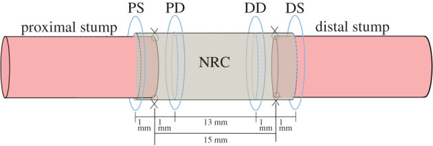
Schematic diagram indicating the nerve repair and NRC geometry, and locations where neurite regeneration are assessed using histological staining. This represents a typical in vivo set-up for assessing nerve injury repair in a rat sciatic nerve model. In the example scenario reported in Georgiou et al. [18], neurite numbers were counted in cross-sections at four locations 1 mm into the proximal (PS) and distal (DS) stumps, or 1 mm into the proximal (PD) and distal (DD) parts of the repair construct, measured from the end of the nerve stump in each case. These data are used to inform the computational modelling framework.
Georgiou et al. [18] counted around 4000 neurites at the PS, of which around 50% made it to the PD after 8 weeks; of these, 70% were recorded at the DD. For the control scenario of an empty tube (no aligned matrix filling), a similar number of neurites made it from the PS to the PD cross-section, but only 10% made it to the DD, as summarized in table 1.
Table 1.
Neurite counts extracted from fig. 4.18 of the work by Georgiou [27].
| repair construct | neurite counts |
|||
|---|---|---|---|---|
| PS | PD | DD | DS | |
| empty tube | 4000 | 2000 | 200 | 200 |
| EngNT | 5000 | 2000 | 1400 | 1000 |
Following the approach in [21], we explore embedding PGFs in an EngNT scaffold to provide an additional directional and stiffness cue to encourage more neurites to reach the DD within eight weeks. First, the provision of parameter values is presented as well as the constitutive relationships in the computational model, using the prescription of the environmental cue term, Pw(t). All parameter values are summarized in table 2.
Table 2.
Summary of the parameters in the computational model. Parameter values are either known based on experimental studies, fitted by comparing model predictions against neurite count data at the sections identified in figure 6 or investigated through a model sensitivity analysis. Finally, the number and radius of the PGFs are determined by optimizing to maximize the number of neurites that reach the DS.
| parameters | definition | value |
|---|---|---|
| γ | growth rate of neurites | 10 µm h−1 [23] |
| δ | standard deviation of growth rate | 0.7 µm h−1 (investigated through sensitivity analysis) |
| n | number of fibres embedded within the NRC | to be determined via optimization |
| r | radius of each of the n fibres | to be determined via optimization |
| N | number of neurites initiated at the PS | 2000 taken from experimental work [18] |
| βV | constant that represents the forward directional bias B(w), when a neurite grows within an empty tube and EngNT | fitted |
| α | thickness of the high-stiffness zone surrounding a PGF | 20 µm [23] |
| kα | the neurite bias to move forward when in the stiffer area surrounding the PGFs | investigated through sensitivity analysis |
| NR | The noise reduction term (equation (2.9)) | fitted |
The duration of simulations (tend), number of neurites simulated (N) and NRC dimensions were fixed based on the experimental protocols described in Georgiou et al. [18]. Next, the function M(θ), which encapsulates the direction of neurite growth in the random walk model (equation (2.5)), was determined based on data from Razetti et al. [6], which reconstructed neurite architectures in three-dimensional from histological staining data of gamma neurites in a Drosophila model. Although the physiology of a Drosophila fly is different to that of a mammal, there is an absence of similar data for mammals available in the literature; further, Fang & Bonini [28] argue that the fundamental mechanisms of axon injury and regeneration are evolutionary conserved. Razetti et al. [6] segmented the Drosophila data providing quantitative data on neurite architecture, with nodes separated by 11 µm as well as measurements of the angles between neurite segments (figure 7). The spacing is approximate to that applied in this model (10 µm). There are several features that cannot yet be compared across species, including the iterative turning angles; however, corresponding three-dimensional datasets are not available for mammals. When such data, in particular for rat nerve repair models, become available, the model could be readily recalibrated.
Figure 7.

Prescription of the PDF M(θ) using data from Razetti et al. [6]. The function M(θ) from equation (2.5) is calculated by fitting a PDF to angle distributions extracted from reconstructed neurite architectures from a Drosophila model by Razetti et al. [6]. Different forms of PDF were tested, with the kernel (bandwidth of 3.58) chosen.
These data were used to inform the function M(θ) by, first, calculating the distribution of angles between neighbouring neurite segments and then fitting different forms of PDF's to the distributions, as demonstrated in figure 7. Normal, logarithmic and kernel distributions were tested, and it is clear that the kernel distribution comprised the sum of normal distributions with a bandwidth of approximately 3.58 best captures the properties of the distribution.
The term Pw(t) in the random walk model (equation (2.5)) encompasses the role of environmental cues in determining the direction of neurite growth on the movement of neurites, including those cues provided by the EngNT (represented by the function B(w), which includes both durotactic and chemotactic effects, and depends on the spatial location through w), and the durotactic cues provided by the fibres (represented by D(k(w)), where k(w) represents the stiffness gradient between the current neurite tip position and those at the following iteration locations, k(w)). Therefore
| 2.10 |
To the best of the authors' knowledge, there are no clear data to inform these relationships directly in the literature. We assume that the baseline chemotactic and durotactic cues present in an empty tube are represented as a constant bias of neurite tips moving towards the distal end of the NRC (βV(w)). The parameter space for βV is informed by ensuring that the forward bias B(w) cannot be larger than the mechanical resistance M(θw), which would result in non-physiological behaviour. As M(θw) has a value between 0 and 1, B(w) is also assumed between 0 and 1, with . For the case of EngNT, the forward bias takes its highest possible value, i.e. B(w) = 1. Subsequently, this constant and the noise reduction parameter are fitted, as described in the following sections, to neurite count data from Georgiou et al. [27] for the empty and EngNT construct (as summarized in table 1).
Finally, the term D(kw) in equation (2.10) describes the response of neurites to the PGF fibres. In [29], the modelling literature describing how cells respond to the stiffness of the ECM is reviewed. These models focus on cell processes at different scales: at the subcellular scale, for example formation of focal adhesion the dynamics of protrusion and stress fibres [30–32], and at the cellular scale, where the main concern is the impact cells have on the structure of the ECM [33,34], or two-dimensional cell motility via durotaxis [24]. The model follows a similar formulation to [26], with the term D(kw) depending on the difference between the stiffness value at the neurite tip at time t (k(wt)), and sum of the stiffness values at all node options for the next time step () and neurite tip location, . Observations from experiments [23] indicate that once a neurite is in close proximity to a fibre, it tends to remain close. Therefore, in the model, neurite tips only respond to increases in durotaxis and ignore decreases (this assumption could be easily changed in the framework, but subsequent sensitivity analysis indicates that model predictions are not highly sensitive to the stiffness parameter)
| 2.11 |
The model incorporates the response of neurites to the stiffness field induced by PGFs. As summarized by figure 8, a zone of depth α (estimated to be approximately 20 µm from experimental observations) is defined where the stiffness bias is modulated by a factor kα. Bhangra [23] observe that when a neurite encounters a fibre, it is biased to remain in the vicinity of that fibre; this is incorporated into the directional cues by reducing the nodes the neurite can move to in subsequent steps. Furthermore, when a neurite is within the distance α from a fibre, its growth rate increases by a factor of two; the implementation of this is explained in later sections. All the effects of a PGF on neurite growth are summarized in figure 8.
Figure 8.
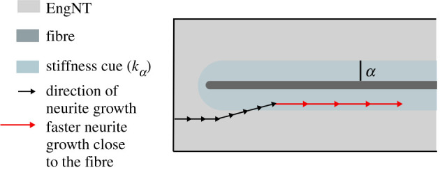
Summary of the impact of a PGF on the growth rate and direction of neurites. The PGFs are embedded throughout the EngNT within the NRC. In a region of depth α around a PGF fibre (depicted in light blue), the stiffness the neurite detects increases compared to the surrounding cellular matrix. Besides providing a directional bias, the region surrounding a fibre also induces a faster growth rate (by a factor of 2).
Parameterization and sensitivity analyses: The model is parameterized (specifically the parameters βV and NR) by comparing its predictions against the neurite count data summarized in table 1. The parameter βV defines the effect of cues (chemotactic, durotactic, etc.) on the neurite growth direction in an empty tube, as well as the increase in these cues when neurites move within EngNT; NR defines the noise reduction. These two parameters are simultaneously optimized for both the empty tube scenario (B(w) = βV) and when in the presence of EngNT (B(w) = 1). The boundaries for the parameter space are summarized in table 3. For all the fitting simulations, the growth rate and standard deviation were kept constant (γ = 10 μm h−1 and δ = 0.7 µm h−1).
Table 3.
The parameter space for data fitting, achieved by comparing model predictions against experimentally measured data on neurite counts at different locations along an NRC.
| parameters | parameter space | reasoning |
|---|---|---|
| βV | 0–1 | chosen to ensure (equation (2.10)) |
| NR | 1–100 | defined ad-hoc |
The parameter space is large (several orders of magnitude); hence, a global optimization algorithm is required. For every parameter combination, the model involves simulating thousands of neurites for hundreds of iterations, requiring an optimization algorithm with a fast convergence rate. The PSO algorithm [35] is quick to converge, does not require computation of derivative terms, or require continuity of the underlying functions. A PSO consists of placing a number of particles (V) distributed throughout the parameter space; at each of these locations, the optimization function is evaluated and compared to neighbouring parameter locations to assess the best (closer to the optimal value) next position, which is perturbed by a stochastic term. The next iteration starts after all particles have moved and progressively all particles move closer to the optimum target values.
Two parameters need to be defined to implement the PSO, which include the number of particles (V) and the maximum number of iterations (G). These need to be chosen to ensure the model converges to the right solution. Here, V was defined as 30 and G was selected in the order of hundreds of iterations.
The error minimized by the PSO algorithm was defined as the error between the experimental neurite count measurements and the equivalent predictions of the computational model. This error metric is calculated for both the empty tube scenario (EH), where B(w) = βV, and the EngNT embedded NRC (EE), where B(w) = 1, simultaneously, and perform the parameterization by minimizing the overall error function (ET), defined as the mean between EH and EE.
Although the PSO algorithm is used for many applications, it has only been shown to work heuristically. The robustness of the PSO outputs are evaluated via the PAWN sensitivity analysis method (Pianosi & Wagener [33]). There are several alternatives to the PAWN, the most commonly used being the Morris method [36]. The Morris method is moment-based and requires many iterations to achieve convergence [37]. By comparison, the PAWN method uses the cumulative density function (CDF) of the model output (y) (here the percentage of neurites that reach the proximal end of the NRC) in order to devise a quantitative measure (PAWN) to apportion the uncertainty of the output to each parameter.
PAWN creates an unconditional CDF (Fy(y)), where all the parameters are varied at random within the ranges established for a number of samples (JU). For each parameter, a number of values (jC) are chosen and nC different CDFs () are constructed for each parameter in turn; for each CDF, a parameter value is chosen and is kept constant, while the remaining parameters are varied randomly over a number of samples (JC). The Kolmogorov–Smirnov (KS) statistic between the Fy and each for each parameter is calculated as
| 2.12 |
The parameters that have the largest KS are the ones that have a more significant impact on the model outputs.
This method is employed to test the sensitivity of the predictions of the model to the parameters: the growth parameter in equation (2.10) (βV), the noise reduction (NR) in equation (2.9), stiffness parameter (kα) in equation (2.11), the depth of the high-stiffness zone surrounding PGFs (α) (algorithm 1) and the standard deviation of the growth rate (δ) (algorithm 2). The parameter ranges chosen are summarized in table 4. Throughout, JU, JC and jC are fixed at 100, 100 and 5 respectfully.
Table 4.
Ranges used to perform the PAWN analysis.
| parameter | range |
|---|---|
| βV | ±20% of the value fitted |
| NR | ±20% of the value fitted |
| kα | 1–3 (dimensionless) |
| α | 10–80 µm |
| δ | ±20% of the value identified in table 2 |
Optimization: We seek to identify the optimal radius (r) and number (n) of fibres embedded within the NRC to ensure the largest number of neurites reach the distal end. Increasing the number of PGFs increases the total cues that promote growth towards the distal stump; however, PGFs also take up space which may become limiting, and therefore optima may be identified. The impact of different numbers of fibres on the behaviour of the neurites in a 100 µm length NRC is illustrated in figure 9, with 5 (figure 9a–c) or 100 (figure 9d–f) embedded PGFs after 0, 5 and 10 h of simulation. The number of neurites that reach the distal stump is approximately 1–3% versus 80% for five versus 100 PGFs, respectively.
Figure 9.

Indicative simulations of neurite growth. Simulations of neurite growth in the presence of five (a,b,c) versus 100 (d,e,f) PGFs, with simulation outputs demonstrated at 0 h (a,d), 5 h (b,e) and 10 h (c,f). Red dots indicate the neurite tip. Fibres were not plotted for the 100 fibre case to aid visualization. The fibre distribution at the proximal stump cross-section was plotted separately to compare the distribution of fibres for the two cases: (g) five fibre case and (h) 100 fibre case. Videos of these simulations can be found in the electronic supplementary material [38].
A PSO algorithm is used again, with parameter ranges for the PGF radius and number prescribed. The minimum PGF radius was based on the feasibility of manufacture (15 µm [23]), and the maximum was set to be the radius of NRC (750 µm). The number of fibres is limited by the number of nodes present in the proximal surface of the mesh (approx. 14 000). For each particle of the PSO algorithm, a value for the two parameters is taken from the ranges described, and the growth of 2000 neurites is simulated for eight weeks.
The error function is dependent on the percentage of neurites that reach the distal stump (against a target of 100%). The PSO was terminated when the improvement between iterations was less than 1%.
Implementation: The model was implemented using the LiveLink package provided by COMSOL to export its mesh building functionalities into Matlab and use it to build the required geometries. All the code was written in Matlab, including the PGF placement algorithm (§2.1), the neurite growth model (§2.2.1) and the PSO algorithm. For the latter, the implementation available in the optimization toolbox from Matlab [35] was used. The PAWN sensitivity analysis algorithm was implemented following examples provided by the work of Pianosis et al. [37].
3. Results
Following the structure of the Methods section, the Results is split into three sections: the fitting of model parameters based on the experimental data presented in table 1, the optimization results for the PGF numbers and radius, and the sensitivity analysis results.
3.1. Parameterization: fitting the model to measured neurite data for both an empty tube and engineered neural tissue
The forward bias parameter (βV) and the noise reduction term (NR) were fitted to the neurite count data from Georgiou et al. [27] (table 1). For these two parameters, the PSO algorithm was run until convergence was achieved, defined as the 30 particles varying by less than 1% from tens of simulations. The result of the fit is presented as box plots in figure 10.
Figure 10.

The PSO algorithm predictions for fitting the parameters βV and NR to the neurite counts for an empty tube and EngNT-filled NRC with no PGFs, based on experimental data on neurite counts summarized in table 1 (from Georgiou et al. [18]). Box plot of the result of the fitted parameters over 30 PSO particles, where the central line is the median, the box encompasses the interquartile range (25th to 75th percentile), the whiskers capture the whole dataset and the red crosses present the outliers, for (a) the βV, that equates the bias of neurites moving towards the distal side of the NRC and (b) NR, the noise reduction parameter.
The robustness of the fit is dependent on the parameter variability, as shown in figure 11, which displays a box plot of the outcome of the 30 particles in terms of the error of the fitting for the individual EngNT embedded (A) and the empty tube NRCs (B). Figure 11 shows that the 30 particles converged to a value, resulting in a quartile range that varies from the mean by approximately 1%. From this range, the mean value (as entered in table 5) was taken forward for subsequent simulations.
Figure 11.

Predictions of neurite regrowth for the parameters identified by the PSO algorithm using the data by Georgiou et al. [18] over 30 particles. Box plot where the central line is the median, the box encompasses the interquartile range (25th to 75th percentile), the whiskers capture the whole dataset and the red crosses present the outliers, for (a) the error for empty tube simulations (b) the mean error for the simulations of an EngNT NRC. Counterpart in vivo measurements are plotted as red lines.
Table 5.
The parameter used in the simulations after fitting them, through the PSO algorithm as seen in figure 10. The values consist in the mean of the 30 particles after conversion.
| parameter | fitted value |
|---|---|
| βV | 0.703 |
| NR | 47.03 |
The values of βV and NR are set as the means of the particle population predicted by the PSO (table 5).
3.2. Optimization: maximizing the number of neurites that reach the distal end of the nerve repair construct through the choice of the number and radius of fibres
Here, the PSO algorithm was run until all the particles converged to a solution where more than 90% of neurites reached the distal stump within eight weeks, and the output of the optimization is compiled over 30 particles. After hundreds of simulations of the PSO, all particles converged to a radius of 15 µm, the smallest considered. The model predicts that packing between 500 and 700 fibres with 15 µm radius within EngNT will result in 91% to 95% of neurites reaching the distal stump within eight weeks (figure 12).
Figure 12.

Outcome of the PSO of the radius and number of fibres, with the variability over 30 particle runs demonstrated. Box plot representing the median and interquartile range (25th to 75th percentile), the whiskers encompass the whole dataset, with the outliers represented by red crosses for (a) the number of fibres embedded in an EngNT NRC and (b) the percentage of neurites that reach the distal end of the NRC.
The PSO algorithm identifies a fibre radius of 15 µm, the smallest manufacturable possible. A comparison of an empty tube or EngNT-filled NRC for an increasing number of 15 µm-radius fibres is shown in figure 13.
Figure 13.

Evaluating how varying the number of 15 µm-radius PGFs for an empty tube and EngNT-filled NRC. Simulations were performed for both conditions by increasing the number of PGFs from 1 to 900. The experimentally measured values for those two conditions without PGFs are plotted as dotted lines.
3.3. Sensitivity analysis: using the PAWN method to understand the impact of varying parameter values on model predictions and the stability of those predictions
The PAWN method is used to quantify the impact of changing parameters summarized in table 4 on the optimal predictions of the model (around 650 fibres with a radius of 15 μm, resulting in 93% of neurites reaching the distal stump in eight weeks). For each nc value, a CDF is constructed, and equation (2.12) is used to identify each KS value, as presented in figure 14.
Figure 14.

Summary of the Kolmogorov–Smirnov statistic for each parameter evaluated. Each dot represents the maximum distance between one conditional CDF (), where the parameter being considered is kept constant and the remaining are varied at random, with the unconditional CDF (Fy(y)) following equation (2.12).
From this analysis, both NR and δ were found to be the parameters with the largest responsibility for the model's predictions. For each parameter, in figure 14, 500 simulations of the model are made. All simulations used to produce the unconditional CDF (Fy) were compiled into a box plot (figure 15) to observe how the number of neurites that reach the distal end of the NRC in eight weeks varies within the parameter space defined by table 4. This clearly demonstrates that for most simulations, the identified number and radius of fibres achieves a higher number of neurites crossing the NRC than the measured value when EngNT is used along without implanted fibres.
Figure 15.
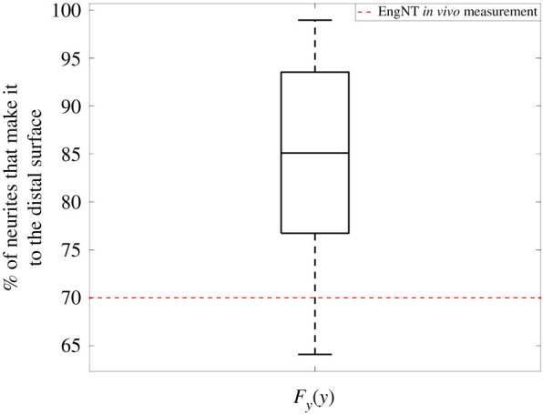
Variability of the number of neurites that reach the distal end of the NRC, when parameters are varied, within the ranges presented in table 4 following the PAWN method. A box plot of all the model outputs that result from the parameter variation encapsulated in the unconditional CDF (Fy(y)), with the median and quartile range (25th to 75th percentile) of the model outputs represented by the box and the whiskers. For comparison, the measured number of neurites that reached the distal end in the EngNT repair model (no implanted fibres) [27] is shown as a dotted red line.
4. Discussion
Here, we discuss the computational framework, its predictions of NRC design, the sensitivity of these predictions to the underpinning parameters and critically analyse the overarching approach.
4.1. Framework
Our computational framework is similar to other literature models [7,39], for example simulating neurites in three-dimensional as lattice-dependent random walks. As with the cited studies, this facilitates the integration of continuous elements into the model, such as soluble factors or therapeutic cells, and this is ongoing at the UCL Centre for Nerve Engineering (for example, as an extension to [16]).
The lattices for lattice-dependent random walks are often comprised of hexahedral elements; these provide a good degree of freedom but present a computational challenge here. An alternative approach was developed where the domain was discretized into equal circles, as seen in figure 3, with the separation between circles and node separation both set at 10 µm (thus matching to the growth rate of the neurites, assuming a time step of 1 h). This approach enables thousands of neurites to be simulated at a millimetre-scale spatial resolution and over a time period of weeks. This lattice-dependent model reduces the number of directions that neurites can choose from at each time step so may increase the chance of neurites getting stuck around fibres; however, similar behaviours have also been observed with non-lattice-dependent models (for example Rizetti et al. [39]).
Both parameterization and optimization of the model were performed using the PSO algorithm. Although this algorithm is commonly used to optimize complex problems in a variety of fields, it does not have a robust theoretical basis (for example, Wang et al. [40] highlight some of the outstanding challenges, including the dependency of the model on its hyper parameters such as the number of particles and their velocities). The use of PSO here is a pragmatic approach; to ensure its predictions are robust, an ad-hoc exploration of model behaviour was performed over the parameter space (figure 13) as well as extensive sensitivity analyses (figure 14).
The data available for parameterization comprise neurite counts at cross-sections through an NRC in rat sciatic nerve models. Using the PSO algorithm, it was possible to match the model predictions to these data. However, the efficacy of the parameterization is sensitive to small changes in parameters, in particular NR and δ (figures 10,11); for example, changing the parameter value by less than 0.5% results in a 3% change in the predicted number of neurites reaching the distal end of the NRC. In order to address this, it is recommended that a future in vivo experiment quantify the number of neurites at several positions within the NRCs and over several time points.
Another set of data, taken from Razetti et al. [39], was used to parameterize the step size for neurite movement and consisted of measurements from a different type of neurite. This dataset was required because of the difference in granularity of scale between the in vivo experiments and the in silico simulations, as the data from Razetti et al. [39] described neurite movements between 10 µm segments. The two sets of data used were acquired from different conditions, different species and different types of neurites.
Regardless, this work demonstrates the feasibility of parameterizing random walk-based computational models of neurite regrowth against data from multiple sources and is flexible to adaptation as further data become available.
Finally, the available data on neurite counts from transverse cross-sections only provide limited information on neurite branching, a known mechanism that neurites employ to sample their environment. The mechanisms that underpin branching and branching rate are subtle to elucidate and have not been fully quantified [7,39]; therefore, branching was not in the model at this stage. It is also unlikely to be a significant determinant of long-term regeneration. Without branching, which tends to be associated with temporary additional sprouts rather than increased functional neurite connections, the predictions of the model may overestimate the efficacy of the approaches under investigation.
4.2. Optimal nerve repair construct design
A PSO algorithm was implemented to optimize the number and radius of the fibres embedded within an NRC fabricated from EngNT. From this analysis, it was found that between 500 and 700 fibres with 15 µm radius should be embedded in EngNT, resulting in a maximum efficacy of 94%.
This result is clearly demonstrated when neurites are simulated for an increasing number of fibres for both empty and EngNT-based NRCs, as seen in figure 13. In both cases, the optimal number of 15 µm fibres was the same. Above 700 fibres, the number of neurites that reach the distal end of the NRC start decreasing, because the fibres start to occupy a larger amount of space. There are no simulations with a number of fibres above 900 because the fibre packing algorithm runs out of space to place them.
Simulations predict that, for the empty NRC, embedding fibres never results in less than 10% efficacy, as seen experimentally, for an empty construct. At approximately, 100–200 fibres the efficacy of the NRC goes beyond the levels associated experimentally with EngNT alone, and a maximum efficacy of 90% is reached, when between 500 and 600 fibres are embedded.
The framework predicts that the number of neurites reaching the distal stump after eight weeks decreases to approximately 60% as the number of fibres increases to around 65–70 (figure 13). This dip is a direct consequence of the concentration of stiffness cues and the model assumption that neurites only move in the direction of higher stiffness, so that neurites congregate around the existing fibres and run out of locations to move to. This effect is replicated in other mathematical models [7,39] and could be addressed by building more complexity into the models once appropriate experimental data are available to inform this.
When the number of fibres embedded in EngNT goes above 100, this provides the cues required to increase the number of neurites that reach the distal end of the NRC, reaching a proportion (94%) similar to that achieved by the PSO algorithm of 94%. This result now needs to be tested experimentally.
Regardless of the number of neurites that cross the NRC, all simulations point to the fibres being as thin as possible (figure 16). Further simulations with 1 μm-radius fibres indicate that the presence of fibres improves outcomes, reaching a maximum efficacy above 95% between 1000 and 2000 fibres and decreasing to approximately zero when the number of fibres approaches 10 000. The optimal value corresponds to a ratio of almost one fibre per neurite. However, all the predictions assume that the radius of the cue surrounding each fibre is kept constant, which has yet to be validated experimentally.
Figure 16.

Predictions of varying the number of 1 µm-radius fibres between 1 and 11 000. Simulations are performed for both an empty and EngNT-filled NRC.
4.3. Robustness of predictions
The PAWN method [41] was used to evaluate the dependence of model predictions on its underlying parameters, chosen as it is not moment dependent and produces graphical outputs of a hierarchy of the parameters. However, Puy et al. [37] have shown that the outputs of the PAWN approach are dependent on how it is parameterized. The limitations of this method can be easily observed when looking at figure 14, where the KS values are evaluated at five points for each parameter at random, leaving the parameter space between those five points unsampled.
Regardless, this method aims to present a hierarchy of the importance of parameter values on the predictions of the model (figure 14). The parameters with a higher KS mean are apportioned a higher responsibility for the observed behaviour in Fy(y). The parameters βV (forward bias), α and kα (stiffness cues surrounding the fibres), are the parameters with the smaller impact, which is explained by the fact that the distribution of stiffness cues is maintained within the parameter ranges chosen. These parameters were informed by observations from Bhangra [23]; however, no direct measurements of the stiffness of the fibres or surrounding region were taken. When further data become available, either on these stiffness measures or on alternative stiffness cues and relationships, these could be readily incorporated into the framework via algorithm 1. The negligible impact of the forward bias on the model is explained by the fact that it is modulated by the noise reduction term NR; hence, although βV makes the probability of moving forward larger than going in any other direction, it does not get chosen if the noise reduction does not allow it.
Further the term B(w) cannot have a higher probability than the M(θ). The sensitivity to NR is clear in figure 14 as the KS value increases when the parameter increases and decreases below the fitted value by 20%. Even when the parameter is varied by 10%, the impact on the model output is larger than most parameters except δ.
The importance of NR underlines the need to uncover the cellular mechanisms responsible for cell motility in response to durotactic cues. Here a simplified model was implemented to ensure the model is manageable; however, when developments are made in this field, the framework presented could easily be adapted.
The PAWN method identified growth rate standard deviation (δ) as the most impactful parameter (figure 14), which will impact the outputs of the model in two ways: (i) neurites will move for a smaller distance for each iteration and (ii) the neurites have less space to move in the case that they share nodes. Alternatively, when increasing α, the impacts on the model inputs are not so extreme, which is explained, in part by the range of values chosen for α and the fact that the spacing between nodes is the same. In summary, when the quantitative measure to evaluate the importance of the different parameters on the predictions of the model is the distance travelled by the neurites, then it is rational that the choice of growth rate will lead to drastic changes in that measure. The model does handle neurites with different growth rates; however, the growth rates need to be multiples of each other in order to use this method for preventing neurites from intersecting. Although this assumption is not realistic in most cases, it has allowed progress to be made and should be expanded in future work.
The PAWN method allows the robustness of the model predictions to be analysed. As seen from the unconditional CDF (Fy(y)) in figure 15, the majority of the simulations (65%) predict that approximately 600 fibres with 15 µm radius will improve the number of neurites reaching the distal end of an EngNT NRC. This should be tested experimentally in future work.
The number of neurites that travel across the two NRCs tested was parameterized using neurite counts from Sprague Dawley rats. The choice of number of neurites at the proximal stump will influence predictions and was investigated (figure 17; these data require re-parameterization of the model as shown in the electronic supplementary material). Neurite growth in response to an increasing number of fibres was explored (figure 17), and a similar trend as in figure 13 was observed. The most crucial prediction is that a maximum proportion of neurites reach the distal stump (around 71%) when around 500 to 900 fibres are used.
Figure 17.

Exploration of varying the number of neurites initiated at the proximal stump on the predictions of NRC efficacy.
The framework developed here demonstrates the potential of using stiff fibres to accelerate regrowth of neurites through an NRC, and more broadly how computational modelling, combined with experimental data, can inform the design of such repair constructs. The next step is to validate predictions of the model presented through in vivo experiments. The approach is dependent on high-quality data from a consistent set of either (or both) in vitro and in vivo experiments and will have most impact when these in vitro, in vivo and in silico studies are co-designed and co-executed.
Data accessibility
All the data used in the paper are available in the electronic supplementary material [38].
Authors' contributions
S.L.: conceptualization, data curation, formal analysis, investigation, methodology, software, validation, visualization, writing—original draft and writing—review and editing; G.P.: methodology and software; K.S.B.: data curation and methodology; J.B.P.: conceptualization, data curation, funding acquisition, project administration, supervision and writing—review and editing; R.J.S.: conceptualization, funding acquisition, methodology, project administration, resources, supervision, writing—original draft and writing—review and editing. All authors gave final approval for publication and agreed to be held accountable for the work performed therein.
Competing interests
We declare we have no competing interests.
Funding
All the research developed was funded by the Engineering and Physical Sciences Research council of the UK (grant no. EP/R004463/1)
References
- 1.Chen S, et al. 2015. Repair, protection and regeneration of peripheral nerve injury. Neural Regen. Res. 10, 1777. ( 10.4103/1673-5374.170301) [DOI] [PMC free article] [PubMed] [Google Scholar]
- 2.Ruijs AC, Jaquet JB, Kalmijn S, Giele H, Hovius SE. 2005. Median and ulnar nerve injuries: a meta-analysis of predictors of motor and sensory recovery after modern microsurgical nerve repair. Plast. Reconstr. Surg. 116, 484-494. ( 10.1097/01.prs.0000172896.86594.07) [DOI] [PubMed] [Google Scholar]
- 3.Scheib J, Höke A. 2013. Advances in peripheral nerve regeneration. Nat. Rev. Neurol. 9, 668. ( 10.1038/nrneurol.2013.227) [DOI] [PubMed] [Google Scholar]
- 4.Pedrosa SS, Caseiro AR, Santos JD, Maurício AC. 2017. Scaffolds for peripheral nerve regeneration, the importance of in vitro and in vivo studies for the development of cell-based therapies and biomaterials: state of the art. In Scaffolds in tissue engineering—materials, technologies and clinical applications, vol. 9 (ed. Baino F). London, UK: IntechOpen. [Google Scholar]
- 5.Angius D, Wang H, Spinner RJ, Gutierrez-Cotto Y, Yaszemski MJ, Windebank AJ. 2012. A systematic review of animal models used to study nerve regeneration in tissue-engineered scaffolds. Biomaterials 33, 8034-8039. ( 10.1016/j.biomaterials.2012.07.056) [DOI] [PMC free article] [PubMed] [Google Scholar]
- 6.Razetti A, Descombes X, Medioni C, Besse F. 2016. A stochastic framework for neuronal morphological comparison: application to the study of imp knockdown effects in Drosophila gamma neurons. In Int. Joint Conf. on Biomedical Engineering Systems and Technologies, pp. 145-166. Berlin, Germany: Springer. [Google Scholar]
- 7.Zubler F, Douglas R. 2009. A framework for modeling the growth and development of neurons and networks. Front. Comput. Neurosci. 3, 25. [cited 2019 Mar 29]. ( 10.3389/neuro.10.025.2009) [DOI] [PMC free article] [PubMed] [Google Scholar]
- 8.Buettner HM. 1994. Nerve growth dynamics. Quantitative models for nerve development and regeneration. Ann. NY Acad. Sci. 745, 210-221. ( 10.1111/j.1749-6632.1994.tb44374.x) [DOI] [PubMed] [Google Scholar]
- 9.Holmquist B, Kanje M, Kerns JM, Danielsen N. 1993. A mathematical model for regeneration rate and initial delay following surgical repair of peripheral nerves. J. Neurosci. Methods 48, 27-33. ( 10.1016/S0165-0270(05)80004-4) [DOI] [PubMed] [Google Scholar]
- 10.Podhajsky RJ, Myers RR. 1995. A diffusion-reaction model of nerve regeneration. J. Neurosci. Methods 60, 79-88. ( 10.1016/0165-0270(94)00222-3) [DOI] [PubMed] [Google Scholar]
- 11.Tse THZ, Chan BP, Chan CM, Lam J. 2007. Mathematical modeling of guided neurite extension in an engineered conduit with multiple concentration gradients of nerve growth factor (NGF). Ann. Biomed. Eng. 35, 1561-1572. ( 10.1007/s10439-007-9328-4) [DOI] [PubMed] [Google Scholar]
- 12.Codling EA, Plank MJ, Benhamou S. 2008. Random walk models in biology. J. R. Soc. Interface 5, 813-834. ( 10.1098/rsif.2008.0014) [DOI] [PMC free article] [PubMed] [Google Scholar]
- 13.Dickinson RB, Tranquillo RT. 1993. A stochastic model for adhesion-mediated cell random motility and haptotaxis. J. Math. Biol. 31, 563-600. ( 10.1007/BF00161199) [DOI] [PubMed] [Google Scholar]
- 14.Smith JT, Tomfohr JK, Wells MC, Beebe TP, Kepler TB, Reichert WM. 2004. Measurement of cell migration on surface-bound fibronectin gradients. Langmuir 20, 8279-8286. ( 10.1021/la0489763) [DOI] [PubMed] [Google Scholar]
- 15.Stokes CL, Lauffenburger DA. 1991. Analysis of the roles of microvessel endothelial cell random motility and chemotaxis in angiogenesis. J. Theor. Biol. 152, 377-403. ( 10.1016/S0022-5193(05)80201-2) [DOI] [PubMed] [Google Scholar]
- 16.Tranquillo RT, Lauffenburger DA. 1987. Stochastic model of leukocyte chemosensory movement. J. Math. Biol. 25, 229-262. ( 10.1007/BF00276435) [DOI] [PubMed] [Google Scholar]
- 17.Schienbein M, Gruler H. 1993. Langevin equation, Fokker–Planck equation and cell migration. Bull. Math. Biol. 55, 585-608. ( 10.1016/S0092-8240(05)80241-1) [DOI] [PubMed] [Google Scholar]
- 18.Georgiou M, Bunting SCJ, Davies HA, Loughlin AJ, Golding JP, Phillips JB. 2013. Engineered neural tissue for peripheral nerve repair. Biomaterials 34, 7335-7343. ( 10.1016/j.biomaterials.2013.06.025) [DOI] [PubMed] [Google Scholar]
- 19.Carvalho CR, Oliveira JM, Reis RL. 2019. Modern trends for peripheral nerve repair and regeneration: beyond the hollow nerve guidance conduit. Front. Bioeng. Biotechnol. 7, 337. [cited 2020 Feb 7] ( 10.3389/fbioe.2019.00337) [DOI] [PMC free article] [PubMed] [Google Scholar]
- 20.O'Rourke C, et al. 2018. An allogeneic ‘off the shelf' therapeutic strategy for peripheral nerve tissue engineering using clinical grade human neural stem cells. Sci. Rep. 8, 2951. ( 10.1038/s41598-018-20927-8) [DOI] [PMC free article] [PubMed] [Google Scholar]
- 21.Kim Y-P, et al. 2015. Phosphate glass fibres promote neurite outgrowth and early regeneration in a peripheral nerve injury model. J. Tissue Eng. Regen. Med. 9, 236-246. ( 10.1002/term.1626) [DOI] [PubMed] [Google Scholar]
- 22.Coy R, Al-Badri G, Kayal C, O'Rourke C, Kingham PJ, Phillips JB, Shipley RJ. et al. 2020. Combining in silico and in vitro models to inform cell seeding strategies in tissue engineering. J. R Soc. Interface 17, 20190801. ( 10.1098/rsif.2019.0801) [DOI] [PMC free article] [PubMed] [Google Scholar]
- 23.Bhangra KS. 2019. Delivery and integration of engineered neural tissue. PhD thesis, UCL, London, UK. [Google Scholar]
- 24.Stefanoni F, Ventre M, Mollica F, Netti PA. 2011. A numerical model for durotaxis. J. Theor. Biol. 280, 150-158. ( 10.1016/j.jtbi.2011.04.001) [DOI] [PubMed] [Google Scholar]
- 25.Aeschlimann M. 2000Biophysical models of axonal pathfinding. Neurocomputing 38–40, 87-92. ( 10.1016/S0925-2312(01)00539-2) [DOI] [Google Scholar]
- 26.Segev R, Ben-Jacob E. 2000. Generic modeling of chemotactic based self-wiring of neural networks. Neural Netw. 13, 185-199. ( 10.1016/S0893-6080(99)00084-2) [DOI] [PubMed] [Google Scholar]
- 27.Georgiou M. 2013. Development of a tissue engineered implantable device for the surgical repair of the peripheral nervous system. See http://oro.open.ac.uk/id/eprint/61175 (accessed 18 Sep 2020).
- 28.Fang Y, Bonini NM. 2012. Axon degeneration and regeneration: insights from Drosophila models of nerve injury. Annu. Rev. Cell Dev. Biol. 28, 575-597. ( 10.1146/annurev-cellbio-101011-155836) [DOI] [PubMed] [Google Scholar]
- 29.Malik AA, Gerlee P. 2019. Mathematical modelling of cell migration: stiffness dependent jump rates result in durotaxis. J. Math. Biol. 78, 2289-2315. ( 10.1007/s00285-019-01344-5) [DOI] [PMC free article] [PubMed] [Google Scholar]
- 30.Harland B, Walcott S, Sun SX. 2011. Adhesion dynamics and durotaxis in migrating cells. Phys. Biol. 8, 015011. ( 10.1088/1478-3975/8/1/015011) [DOI] [PMC free article] [PubMed] [Google Scholar]
- 31.Kim MC, Kim C, Wood L, Neal D, Kamm RD, Asada HH. 2012. Integrating focal adhesion dynamics, cytoskeleton remodeling, and actin motor activity for predicting cell migration on 3D curved surfaces of the extracellular matrix. Integr. Biol. 4, 1386-1397. ( 10.1039/c2ib20159c) [DOI] [PubMed] [Google Scholar]
- 32.Kim MC, Whisler J, Silberberg YR, Kamm RD, Asada HH. 2015. Cell invasion dynamics into a three dimensional extracellular matrix fibre network. PLoS Comput. Biol. 11, e1004535. ( 10.1371/journal.pcbi.1004535) [DOI] [PMC free article] [PubMed] [Google Scholar]
- 33.Schwarz US, Bischofs IB. 2005. Physical determinants of cell organization in soft media. Med. Eng. Phys. 27, 763-772. ( 10.1016/j.medengphy.2005.04.007) [DOI] [PubMed] [Google Scholar]
- 34.van Oers RF, Rens EG, LaValley DJ, Reinhart-King CA, Merks RM. 2014. Mechanical cell-matrix feedback explains pairwise and collective endothelial cell behavior in vitro. PLoS Comput. Biol. 10, e1003774. ( 10.1371/journal.pcbi.1003774) [DOI] [PMC free article] [PubMed] [Google Scholar]
- 35.Eberhart R, Kennedy J. 1995. Particle swarm optimization. In Proc. of the IEEE Int. Conf. on Neural Networks, Perth, WA, Australia, 27 Nov.-1 Dec., pp. 1942-1948. Piscataway, NJ: IEEE. [Google Scholar]
- 36.Campolongo F, Braddock R. 1999. Sensitivity analysis of the IMAGE Greenhouse model. Environ. Model. Soft. 14, 275-282. ( 10.1016/S1364-8152(98)00079-6) [DOI] [Google Scholar]
- 37.Puy A, Piano SL, Saltelli A. 2019. A sensitivity analysis of the PAWN sensitivity index. arXiv preprint arXiv:190404488. ( 10.1016/j.envsoft.2020.104679) [DOI]
- 38.Laranjeira S, Pellegrino G, Bhangra KS, Phillips JB, Shipley RJ. 2022. In silico framework to inform the design of repair constructs for peripheral nerve injury repair. Figshare. [DOI] [PMC free article] [PubMed] [Google Scholar]
- 39.Razetti A, Medioni C, Malandain G, Besse F, Descombes X. 2018. A stochastic framework to model axon interactions within growing neuronal populations. PLoS Comput. Biol. 14, e1006627. ( 10.1371/journal.pcbi.1006627) [DOI] [PMC free article] [PubMed] [Google Scholar]
- 40.Wang D, Tan D, Liu L. 2018. Particle swarm optimization algorithm: an overview. Soft. Comput. 22, 387-408. ( 10.1007/s00500-016-2474-6) [DOI] [Google Scholar]
- 41.Pianosi F, Wagener T. 2015. A simple and efficient method for global sensitivity analysis based on cumulative distribution functions. Environ. Model. Soft. 67, 1-11. ( 10.1016/j.envsoft.2015.01.004) [DOI] [Google Scholar]
Associated Data
This section collects any data citations, data availability statements, or supplementary materials included in this article.
Data Availability Statement
All the data used in the paper are available in the electronic supplementary material [38].