Monitoring LITT thermal penetration depth using real-time analysis of backscattered light

Abstract

Real-time monitoring of the thermal penetration depth (TPD) is essential in various clinical procedures, such as Laser Interstitial Thermal Therapy (LITT). MRI is commonly used to this end, though bulky and expensive. In this paper, we present an alternative novel method for an optical feedback system based on changes in the diffused reflection from the tissue during treatment. Monte-Carlo simulation was used to deduce the relations between the backscattered pattern and the TPD. Several methods of image analysis are developed for TPD estimation. Each yields a set of parameters which are linearly dependent on the TPD. In order to test these experimentally, tissue samples were monitored in-vitro during treatment at multiple wavelengths. The SNR and coefficient of determination were used to compare the various methods and wavelengths and to deter-mine the preferred method. Such system and algorithms may be used for real-time in-vivo control during laser thermotherapy and other clinical procedures.

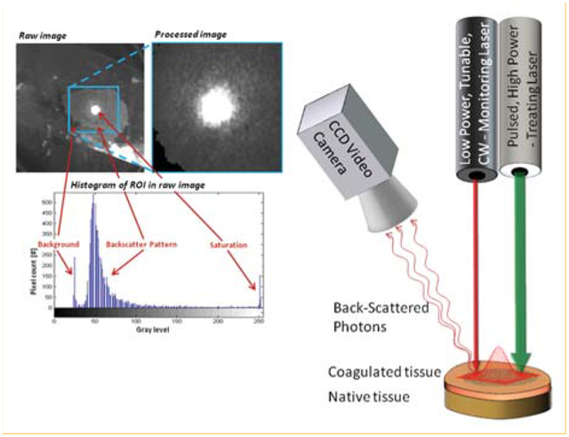
Setup (right) and image analysis (left) preformed on tissue sample for estimation of the Thermal Penetration Depth (TPD).

Graphical Abstrat

1. Introduction

Laser Interstitial Thermal Therapy (LITT) is a surgical procedure for thermal therapy in small volumes of soft tissue. This method is frequently used for era-dicating small, non-metastatic tumors, such as hepa-tocellular cancer or neoplasms in the brain and spinal cord [1, 2]. When the tumors are localized, LITT is superior to common chemotherapy or radiation therapy, since its effects are restricted to the tumor site without any systemic effects. By inserting thin, flexible optical fibers into the tumor sites, LITT allows for a minimally invasive thermal treatment of a specific area, with minimal damage to the surrounding healthy tissue [3, 4]. Thus, the major advantage in using LITT over traditional surgical procedures is when a surgical intervention might be complicated and/or risk the patient [1]. In addition, in order to achieve complete thermal eradication of the tumor sites while minimizing the damage to the surrounding healthy tissue, a real-time intra-operative monitoring of the thermal penetration depth (TPD) is required during the laser operation [1, 3, 5–7]. Such a method should be fast and accurate enough to prevent unnecessary damage.

Currently, the clinical method commonly used for monitoring LITT is MRI, which provides a three-dimensional, real-time monitoring system of thermal effects and the evaluation of treatment-induced coagulation necrosis. Furthermore, MRI enables a good distinction of temperature changes smaller than 1 °C. However, MRI is a costly method and requires a highly skilled interventional radiologist, and therefore has low accessibility [1, 2].

Other clinically accepted methods for monitoring LITT are Ultrasound Imaging and Computerized To-mography (CT-Scans) [1, 2, 4, 8–10]. These methods have either inferior resolution to MRI or involve large doses of ionizing radiation. Hence, they are usually used when MRI is not possible, unavailable, or when there are medical limitations on using MRI [1, 2, 4, 5, 10].

In the past, several research works suggested using the IR thermal radiation emitted from the tissue for monitoring various laser treatments, such as skin resurfacing by CO₂ laser [6, 7, 11, 12]. These methods are based on collecting the IR thermal radiation emitted from skin layers (i.e. using an IR photonic detector coupled with a silver halide optical fiber) and infer the TPD based on thermal damage models. Such a method was applied for estimating the burns TPD by a simple linear equation [6]. The thermal methods mentioned above suffer from low accuracy and slow acquisition times, due to the indirect measurement of coagulation through the diffusive propagation of heat [12].

In recent years, optical methods in the visible and near-IR range were offered for measuring the TPD [3, 7]. In particular, it was shown that there is a linear relation between the TPD and reduced scattering coefficient ${\mu }_s^{\prime }$ [3]. In order to monitor the LITT process, the power of the back-emitted mid-IR radiation was temporally resolved. In an alternate configuration, a secondary low-power laser was used to illuminate the tissue, and the backscattered light was collected using a CCD camera. The spot size backscattered pattern was then used to estimate the TPD. No spatial analysis of the backscattered pattern was performed.

A comprehensive, multi-wavelength analysis of the spatial distribution of light was never carried out and may hold the key for a fast, accurate and simple mechanism of monitoring LITT. Moreover, since the scattering coefficient is wavelength-dependent [13–16], so is the backscattering pattern. Therefore, illuminating the tissue with several low-power lasers at different wavelengths and analyzing several images of a specific situation may improve the backscattering analysis and allow for more accurate estimation of the TPD.

To this end, a low-power tunable laser source and multiple image processing algorithms were used, utilizing the linear relation between the reduced scattering coefficient and the TPD. Rapid estimation of the TPD online was obtained by using a video CCD camera to measure changes in the tissue’s backscattering pattern. Several image processing algorithms were tested for the analysis of the backscattering, both theoretically and experimentally, in order to find an optimal combination of monitoring lasers, wavelengths and algorithms.

2. Method and materials

2.1. Monte-Carlo simulation

First, we theoretically analyzed the spatial distribution of the backscattered light.

A Monte-Carlo simulation of Multi-Layered Medium (MCML) was used to simulate the diffused reflectance pattern as a function of the radial distance from the beam center [17]. The simulation was used to estimate backscattering changes, due to structural changes caused by LITT. A monitoring laser of 633 nm wavelength with Gaussian beam profile (0.2 cm width, 5 J maximum intensity) was used. The simulated tissue was composed of two layers; The upper, thin layer simulated the treated layer of the tissue, which was coagulated after being exposed to the treating laser. The lower, thicker native layer simulated the tissue unaffected by the laser. The simulation parameters are described in Table 1. Different thicknesses of the coagulated layer were tested, ranging from 0.1 mm to 2 mm in, steps of 0.1 mm. This range was chosen in accordance with previous works [3, 7, 13]. The scattering coefficient of the coagulated tissue layer was increased linearly, respective to the increase in the coagulated layer’s thickness. This was shown in the works of Gannot et al. and Ai-ping Qian et al. [3, 10].

Table 1.

MCML simulation parameters. The laser wavelength is 633 nm with a 5 J Gaussian beam profile (0.2 cm width). The thickness of the upper coagulated tissue layer (dubbed d₁) varies from 0.1–2 mm with 0.01 cm increments. The scattering coefficient of the coagulated tissue varies linearly, respective to layer thickness.

Layer	Thickness d [cm]	Refractive index n [#]	Anisotropy factor g [#]	Absorption coeff. μa [cm−1]	Scattering coeff. μs [cm−1]
Coagulated Tissue	d1 = 0.01 to 0.2 (0.01 increments)	1.37	0.927	0.12	228 + 912 ⋅ d1
Native Tissue	1 - d1	1.37	0.965	0.12	228

The output of each simulation was presented in a simulated diffused reflectance map. Each radial reflectance map was fitted with a radial Gaussian function, as shown in Eq. (1):

$$\widehat{R}\left(r\right)=A_r{\text{e}}^{-\frac{1r^2}{2{\sigma }_r^2}}$$ (1)

Both the radial amplitude A_r and the radial standard deviation σ_r were analyzed as a function of the coagulated layer thickness. In addition, variance of the backscattered intensity was estimated using Eq. (2):

$$V_{a}r\left(\widehat{R}\right)=\frac{1}{S_{\text{image}}}\int \int {\left(\widehat{R}\left(r\right)-\overline{R}\right)}^2\text{d}s$$ (2)

where the integration is assumed over the entire image. S_image is the area of the image and $\overline{R}$ is the mean backscattered intensity. Each of these quantities serves as a measure of the Thermal Penetration Depth.

In order to verify whether changes in the backscattering are related to the increase in scattering coefficient or to the varying thickness of the coagulated tissue (which corresponds to the Heat Penetration Depth), additional simulations were performed with either a constant tissue thickness or a constant scattering coefficient. Results were analyzed, as described above. The dependence of each measure of the TPD on either the coagulated tissue thickness or the scattering coefficient was calculated.

2.2. The experimental setup

The experimental setup is shown in Figure 1 below. In order to measure the influence of heating on the backscattered light pattern, chicken breast samples were used. Chicken breast tissue was chosen due to the simplicity of cutting and preparing it, good contrast images and the resemblance of its optical properties [18] to certain human tissues treated in LITT (such as human breast).

Figure 1.

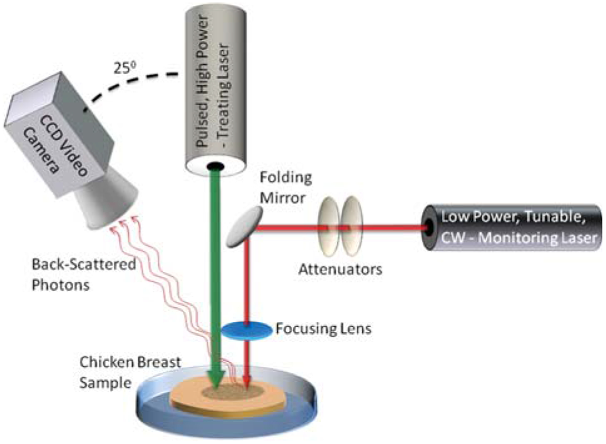
The experimental setup. A pulsed high-power laser is focused on a chicken breast tissue sample to generate the LITT process. In addition, a low-power monitoring laser is aimed at the tissue sample as well. A CCD video camera is used to capture the backscattered pattern from the monitoring laser irradiation.

The experimental setup included a high-power CO₂ laser (Lumenis, Sharplan 1055 s, Yokneam, Israel), irradiated on the tissue to generate the LITT process. Power and pulse duration were set to 5 W and 1 second, respectively. Exposing the tissue to a single pulse resulted in a small change to the backscattering. Therefore, each tissue sample was exposed to an increasing number of pulses, ranging from 2 up, until carbonization occurred after 14 pulses.

An additional low-power, CW, tunable laser was used simultaneously with the treating laser in order to generate the backscattered speckle pattern which was then analyzed. Two different laser sources were used: Helium-Neon (Melles-Griot 05-LHP-151) lasing at 633 nm, and tunable Ti: Sapph laser (Spectra physics model 3900S) lasing at 750 nm, 800 nm and 850 nm. The laser was coupled with the tissue sample using a set of Broadband Dielectric Mirrors (Thorlabs, BB1-E02) and a biconvex AR coated lens (Thorlabs, LB1757-B). Two laser Attenuators (Thorlabs, NE20B and ND01B) were used to adjust the laser intensity and diminish most of the saturation effects. Though saturation decreases the amount of information in the image, a small amount of saturation in the central region of the speckle pattern was desirable; That, due to the fact that a small increase in the intensity of the diagnostic laser (which causes a small amount of saturation) significantly increased the signal to noise ratio in the mid and peripheral regions of the speckle pattern.

The backscattered light from the tissue was collected by a video-rate CCD camera (Cohu 2100 – monochrome solid state camera, CCIR format). The camera was positioned in 25° with respect to the laser beam. The distance between the camera and the sample was approximately 30 cm.

The entire experiment was performed several times. Each time, a different set of tissue samples and a different monitoring laser wavelength were used (about five sets for each monitoring wavelength).

3. Image processing methods to estimate thermal depth penetration

Several algorithms for analyzing the backscattered light images and simulation results were developed. Each algorithm examines a different parameter of the image, which changes consistently with the number of laser pulses.

3.1. Pre-processing

In the first stage, undesired background objects were removed from the images, using an automatic algorithm. The algorithm is based upon cropping the Region of Interest (ROI) in the image, followed by zeroing the residual undesired regions. Residual background objects were identified and excluded based on the multimodality of the grayscale distribution in the image. The bright backscattered pattern is ascribed with higher grayscale values, while un-illuminated background objects are ascribed with lower grayscale values. The process is shown in Figure 2. Automatic background removal is important, since it allows us to bring all images to a common ground and analyze them on the same footing.

Figure 2.

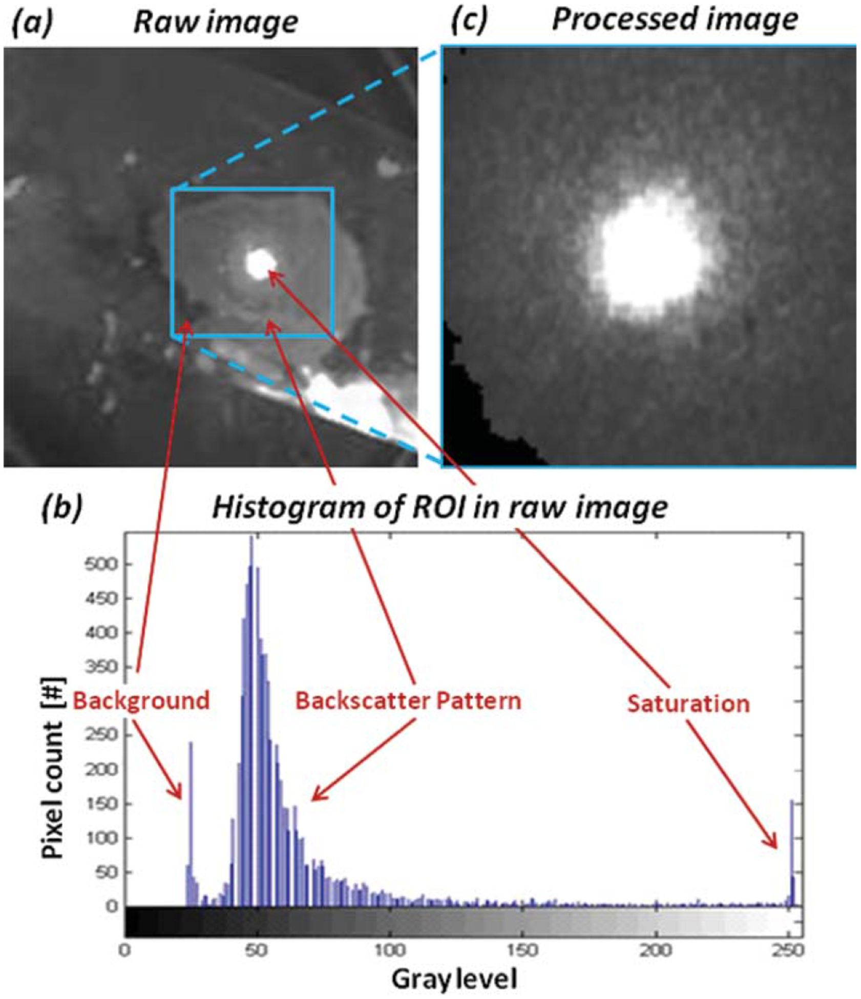
(a) A typical raw backscattering image captured during experiments. (b) Based on the raw image histo-gram, a square region of interest, which contains primarily the saturation and backscatter pattern, is selected and cropped. (c) Residual pixels of the background are then excluded from the processed image (shown in black in the left bottom corner of (c)).

3.2. Algorithms for evaluation of the thermal penetration depth

The first algorithm consists of calculating the variance of grayscale values in the image. As the LITT procedure progresses, the scattering coefficient increases [4, 10]. Thus, the backscattered speckle pattern should display higher fluctuation [3]. Therefore, an increase in the scattering coefficient will reduce the homogeneity of the backscattered intensity and increase the variance of grayscale values in the image. Variance was calculated for either the backscatter pattern pixels or both saturation and backscatter pattern pixels.

A second algorithm was based upon the area of backscattered pattern. Calculation of the area was achieved by applying a threshold to binarize the images, followed by fitting of an ellipse to the binarized image. Binarization of the images was performed with three different constant thresholds. Different thresholds were used in order to find an optimal threshold value.

In order to fit the data with an ellipse, we first binarized the image. Noise was removed by identifying all connected components and removing those of small areas. Then, the boundaries of the binary shape were traced and a circle was fitted in order to find the minor radius of the ellipse, as shown in Figure 3. The major radius was found by Radon transform. The point of maximum intensity in the Radon image corresponds to the angle and offset of the longest line in the binary image, which is the major radius of the ellipse. The ellipse area was then calculated by multiplication of the radii times π.

Figure 3.

Algorithm for calculating the area of the backscattered pattern by fitting an ellipse; The image is binarized and noise is removed. Then, the boundaries are traced and a circle is fitted to find the minor radius. Radon transform is used to find the major radius. Finally, an ellipse is fitted and its area is calculated by multiplication of the radii times π.

This area is expected to grow with the sample’s scattering coefficient, due to the shortening of the transport mean path between scattering events: $l_s^{\prime }=1/\left[\left(1-g\right){\mu }_s\right]$ Therefore, photons traveling inside the tissue encounter a higher number of scat-terers per unit length and the “banana-like” photon path is shorter. Since more photons escape the tissue closer to the incident laser beam, the central region has higher peak intensity, and consequently the ellipse area for a given threshold is larger (given the threshold is high enough).

Finally, it is important to notice that the anisotropy between axes is mostly related to the beam shape of the laser and the angle of the camera, rather than to the anisotropy of the sample.

The third algorithm consists of fitting a spatial function to the observed data. Based on our theoretical simulation trails, we assumed the intensity profile of the backscatter pattern resembles a Gaussian function. In order to reduce the number of fitted parameters, each image was rotated to the camera frame of reference, using Radon transform, as described earlier. In the camera frame of reference, the spatial Gaussian function is dependent upon five scalar parameters, described by the following equation:

$$\widehat{R}\left(x,y\right)=A_{xy}{\text{e}}^{-\frac{1}{2}\left(\frac{{\left(x-x_0\right)}^2}{{\sigma }_x^2}+\frac{{\left(y-y_0\right)}^2}{{\sigma }_y^2}\right)}$$ (3)

where A_xy is the peak intensity, x₀, y₀ are the x and y coordinates of the peak location and σ_x, σ_y are standard deviations in the x and y direction, respectively. Each image was fitted to the spatial Gaussian function. Peak intensity, peak position and standard deviations were calculated. As the treatment process progressed and the scattering coefficient grew, we expected the standard deviations to decrease and the peak intensity to increase; this, for the same reason discussed earlier regarding the ellipse area method.

4. Results

4.1. Monte-Carlo simulation results

Based on the radial diffuse reflectance maps of the simulation, variance of the backscattered intensity was calculated for each coagulated tissue layer thickness. Figure 4a presents the variance calculated for thicknesses ranging from 0.01 cm to 0.2 cm. It is clearly seen that the variance increases linearly in respect to the depth of the coagulated layer.

Figure 4.

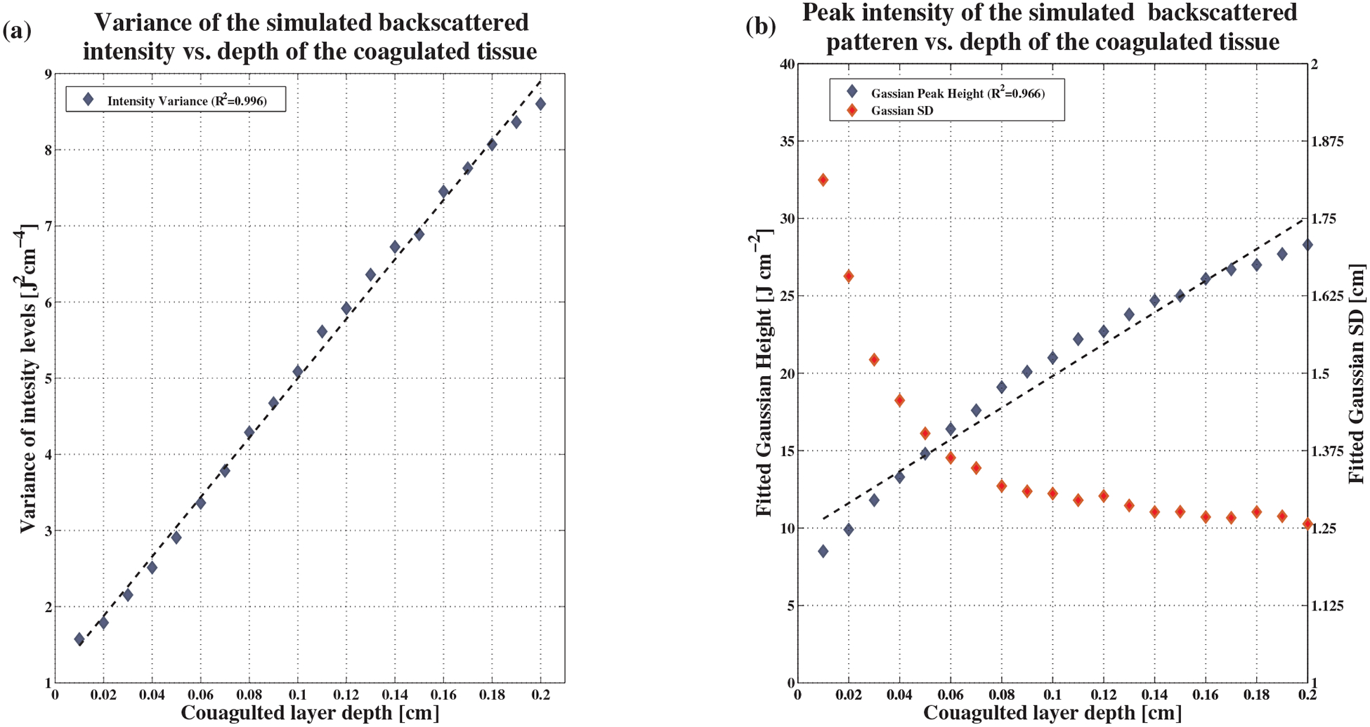
Simulation results. (a) Variance of backscattered intensity as a function of the coagulated layer thickness. The coefficient of determination to a linear fit is 0.996. (b) Peak and standard deviation of the backscattered intensity, also shown as a function of the coagulated layer thickness. The coefficient of determination for peak intensity is 0.966. For standard deviation, the linear fit is poor and thus not shown in this Figure.

A high coefficient of determination R², 0.996, was attained. In addition, a radial Gaussian function was fitted to the simulated backscatter maps. Gaussian fitting was found to be a very accurate estimate of the simulated backscatter maps, with an average error of fitting as small as 1.5%. The Gaussian peak height and the standard deviation in each coagulated tissue layer thickness were calculated. Results are shown in Figure 4b. It is evident that the Gaussian height grows linearly as the depth of the coagulated layer increases. The coefficient of determination attained was again high, 0.966.

In contrast, the Gaussian’s standard deviation, though decreasing as expected, did not exhibit any linear behavior. The coefficient of determination for linear fitting was very low (about 0.6). Therefore, the fitting is not shown in Figure 4b.

To further investigate the effects of changes in the scattering coefficient on TPD measures, we simulated a set of synthetic scenarios. Thickness of the coagulated tissue varied, while the scattering coefficient was held constant at different values. The same was performed for constant thicknesses, while the scattering coefficient varied. Variance of the backscattered intensity and peak intensity for a fitted Gaussian function were calculated for each scenario. The dependence of each measure on the coagulated tissue thickness (which corresponds to the TPD) or on changes in the scattering coefficient was calculated using linear regression. Results are presented in Figure 5a–d. These results provide some insight into the machinations of the suggested measures. It is apparent that the derivatives of both measures with respect to the coagulated tissue thickness are a thousand fold larger than those with respect to the scattering coefficient. However, multiplying those derivatives in the appropriate parameter ranges (as shown in Figure 5) we see that the dependence of the variance measure on the coagulated tissue thickness is only 1.45 to 2.25 times greater then it’s dependence on the scattering coefficient. For the peak intensity measure, the dependence on the coagulated tissue thickness is only 1.25 to 1.35 times greater then it’s dependence on the scattering coefficient. Thus, both measures are sensitive to changes in the scattering coefficient, independent from the coagulated tissue thickness. This might seem to suggest that the scattering coefficient should be estimated in addition to the TPD (as nuisance parameter) to negate the strong dependence of these measure in it. However, it was shown that for the LITT process, the scattering coefficient itself has a strong positive correlation to the TPD [3, 4, 10]. This shows, at least on pure theoretical grounds, that these measures are adequate for TPD estimation as they are sensitive to parameter strongly correlated with the TPD. Finally, the dependence on the coagulated tissue thickness shows a mild deviation from linearity in thick tissues. This restricts the range of applicability to a linear estimator, as presented in this research. In order to extend the usefulness of these measures, a non-linear relation between the TPD and the calculated measure must be assumed, and is beyond the scope of this work.

Figure 5.

Synthetic simulation results. (a) Variance of backscattered intensity as a function of the coagulated layer thickness, for a constant scattering coefficient. (b) Peak of the backscattered intensity as a function of the coagulated layer thickness, for a constant scattering coefficient. (c) Variance of backscattered intensity as a function of the scattering coefficient, for a constant coagulated layer thickness. (d) Peak of backscattered intensity as a function of the scattering coefficient, for a constant coagulated layer thickness.

4.2. In-vitro experiment results

The algorithms discussed earlier were applied to the images of chicken breast tissue samples exposed to an increasing number of pulses.

Using the first algorithm, variance was calculated with and without the saturated area. Figure 6a shows an example of the results for a wavelength of 800 nm with a 90% confidence interval (mean ± 1.645 standard error). As can be seen, variance increases linearly as the number of pulses increase. The coefficient of determination obtained by including or excluding the saturated area is very similar. However, calculating the variance including the saturated area was shown to be less sensitive to experimental conditions, and results are more repeatable.

Figure 6.

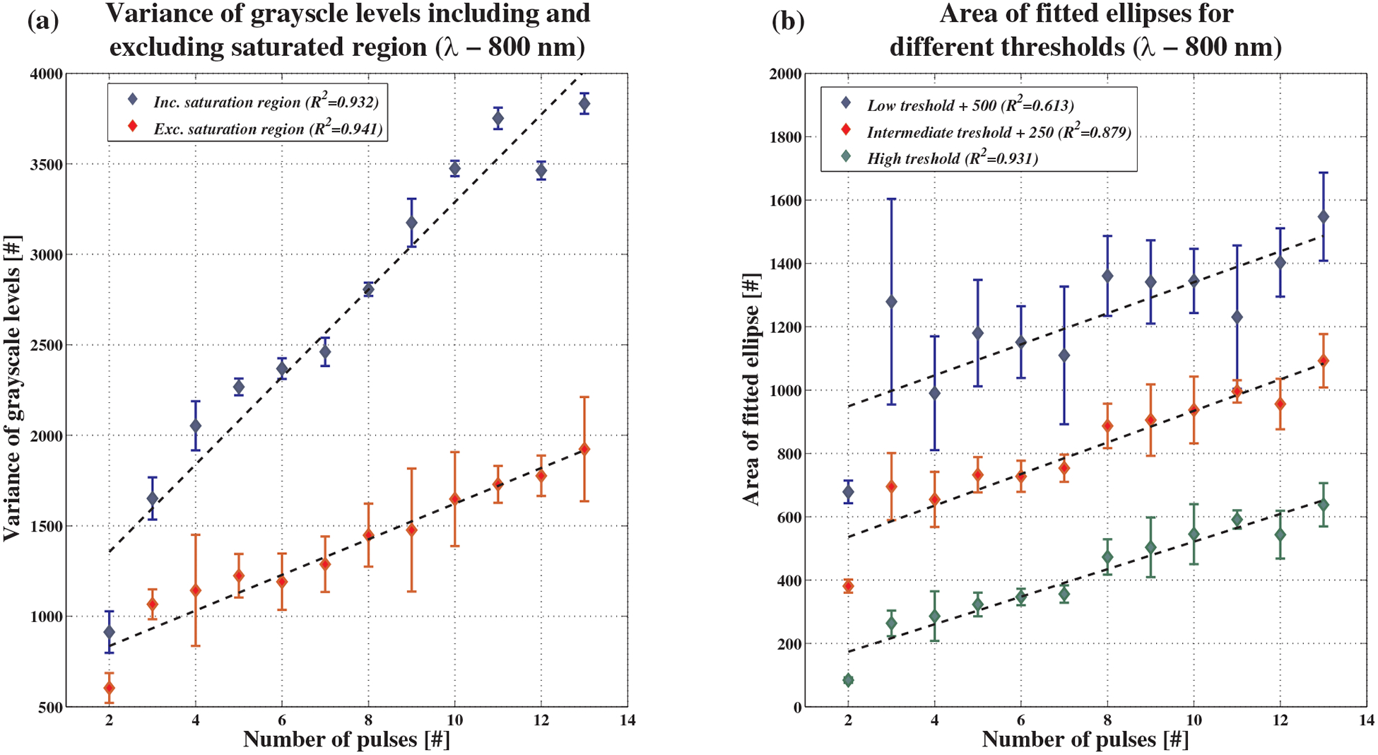
Experimental results for intensity variance and ellipse area algorithms at 800 nm. (a) Variance of the grayscale intensities. Variance was calculated including and excluding the saturated area in the center of the backscatter pattern. A linear fit was then applied with coefficient of determination ranking from 0.932 to 0.941, respectively. (b) Ellipse areas for one set of measurements. Ellipses were measured on a binary image created using 3 different gray level thresholds: 100 (R² = 0:613), 150 (R² = 0:879) and 200 (R² = 0:931). For presentation purposes, constant values of 500 and 250 were added to the lower and intermediate thresholds.

For the second method of calculating the ellipse area, three different gray level thresholds were used – 100, 150 and 200. These thresholds were chosen arbitrarily to span a reasonable range of threshold options. Figure 6b shows an example of the results, again for 800 nm. To separate between graphs (for reader’s convenience), constant values of 500 and 250 were added to the ellipse areas with lower and intermediate thresholds, respectively. As expected, there was an increase in the ellipse area as the number of laser pulses increased. It is apparent that using a higher threshold is preferable, since the resultant ellipse area grows more consistently with the number of laser pulses. In addition, a higher threshold is more robust and has a smaller error range, due to the removal of all background artifacts.

Finally, the spatial Gaussian algorithm was tested. Figure 7 shows an example for 633 nm. The Gaussian peak value and standard deviations in both axis (σ_x & σ_y) are plotted as a function of the number of CO₂ laser pulses. Again, 90% confidence intervals were plotted. In Figure 7b, a constant value of 5 was added to the y-axis standard deviation, separating the graphs for a more convenient presentation. Figure 7a and b show that as the number of pulses increase, peak value of the fitted Gaussian increases and standard deviations decrease. These results coincide with the theory explained above. However, as opposed to simulation results, the measured values exhibit linear behavior, thus yielding high coefficients of determination when fitted to linear functions.

Figure 7.

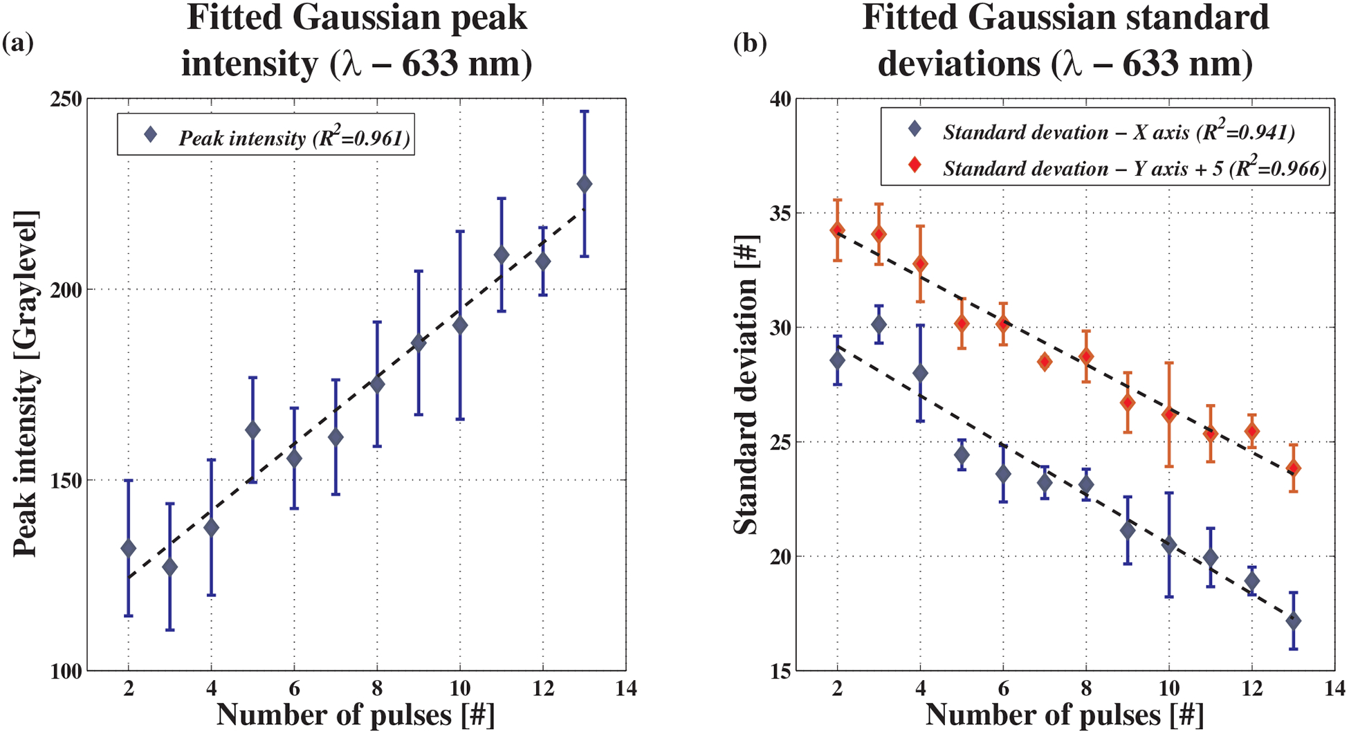
Experimental results for the spatial Gaussian algorithm at 633 nm. (a) Gaussian peak height as a function of the number of pulses. Coefficient of determination is 0.961. (b) Gaussian standard deviations in the x and y axis. Coefficients of determination are 0.941 and 0.966, respectively. For convenience, constant values of 5 were added to the y-axis standard deviations in order to separate the graphs.

For comparison between methods, a measure of the methods’ quality was defined. The Q-factor was defined as:

$$Q=\frac{A}{\langle \sigma \rangle }$$ (4)

where A is the slope of linear fit, proportional to the method’s sensitivity, and $\langle \sigma \rangle$ is the average standard deviation of the measurement for this method (proportional to the noise of the measurements). Thus, the Q-factor is a measure of Signal to Noise Ratio (SNR). Results are summarized in Table 2 below.

Table 2.

In-vitro experimental results summary. For each method tested and for each wavelength used in the experiments, the coefficient of determination and Q-factor are presented. The wavelength of highest SNR (averaged over methods) is marked with a solid color. The method that achieved highest SNR (averaged over wavelengths) is marked with dots. The combination of wavelength and method that achieved highest SNR is marked with diagonal lines.

As can be seen in Table 2, the method yielding maximal SNR (averaged over wavelengths) is the fitting of a spatial Gaussian and measurement of its peak intensity. The preferable wavelength is 800 nm, yielding both highest SNR and excellent linear fitting for most tested parameters. However, the combination of method and wavelength that exhibited the highest SNR is the variance method (including or excluding the saturated area), for a 800 nm wavelength.

5. Discussion

In this research, various methods for real-time monitoring of the LITT Thermal Penetration Depth (TPD) were analyzed. Monitoring was based on illumination of the tissue with additional low-power lasers at multiple wavelengths, and analyzing of the backscattered light. Various algorithms for estimation of TPD during laser surgery were investigated, using both theoretical Monte Carlo simulation and in-vitro experiments on chicken breast tissue samples. It was demonstrated that using an 800 nm diagnostic laser, combined with a simple automatic image processing algorithm (including pre-processing followed by calculation of the image variance or fitting of a spatial Gaussian function) can yield a fairly accurate estimate of the number of laser pulses to which the tissue was subjected with high SNR. The number of pulses is directly proportional to the TPD, as shown in previous works of Gannot et al. [3]. Thus, the actual TPD can be estimated by a simple linear relation. Working at 800 nm allowed for deep penetration into the tissue, and high precision of TPD estimation for a wide range of depths.

Results of the MCML simulation show that, in a noise-free environment, both fitted Gaussian peak height and variance method are very sensitive to the TPD. The fitted Gaussian standard deviation sensitivity to the TPD is at least one order of magnitude less than the variance method. This suggests that the standard deviation is a less suitable measure of the TPD. The simulation also shows the highly linear behavior of the fitted Gaussian peak height and the variance method over a wide range of TPDs. These results correlate with the in-vitro experiments. However, the simulation fails to predict the linear behavior of the standard deviation that was experimentally observed. This might be due to the erroneous representation of the coagulated tissue geometry. Due to the nature of the tissue’s thermal interaction with the treating laser, it is reasonable to assume that the coagulated tissue geometry is roughly the shape of a hemisphere [3]. However, the MCML simulation assumes an infinite number of tissue slabs of variable depths. Thus, small changes in the scattering properties of the tissue, which in reality are confined to a small local volume, affect the entire infinite tissue slab, thus profoundly changing the backscattered pattern. In the in-vitro experiments, the changes in each parameter were smaller and remained linear until tissue carbonization was reached. Thus, the simulation results are an overestimation of the real results and should only be interpreted qualitatively, as an upper bound for the system’s performances. In order to better estimate the effects of coagulation on the backscattered pattern, a specialized Monte-Carlo simulation should be developed, taking into account the complex geometry of the laser-irradiated tissue.

Though qualitative, simulation results prove their value by providing insight into the underlying machinations to the generation of a backscattering signal. Using a theoretical model, we have shown that the backscattered intensity, and consequently the suggested measures of the TPD have similar dependence upon depth and scattering coefficient of the coagulated tissue. Since both increasing with the progression of treatment, results have shown that the suggested measures of the TPD provide a good estimation of the TPD on their own and no nuisance parameters should be estimated. Another insight gained concerns the non-linearity of the TPD measures for large depths. With the increase of the coagulated tissue depth, the number of photons reaching the unaffected tissue and scattering back to the surface decreases. Thus, the sensitivity of the backscattered intensity to the coagulated tissue depth decreases for large TPD values. This poses a limit on the range of TPD that can be estimated using the proposed method.

Experiments show that the best results are achieved at a 800 nm wavelength. For this wavelength, there is minimal absorption for all primary tissue constitutes: water, lipids, Oxy-Hemoglobin (O₂Hb) and Deoxy-Hemoglobin (HHb). Thus, the penetration of light is the deepest. In shorter wavelengths, the absorption of hemoglobin can be substantial. Such absorption decreases backscattering and lowers the SNR. Moreover, the scattering coefficient of a tissue in the visible and near-IR ranges is known to decrease with shorter wavelengths. Thus, for longer wavelengths, the SNR is again decreasing. The Gaussian peak height was shown to have a good SNR and highly linear behavior over all wavelengths tested. This method is fairly simple and has a low sensitivity for the camera alignment and lighting conditions. Therefore, it provides a robust estimate of the TPD. The variance method at 800 nm was proven to have exceptionally high performances. However, its performances at other wavelengths are lacking. This raises doubts regarding its applicability to monitor the TPD. It seems that the reason for this inconsistency is the method’s sensitivity to slight variations in lighting conditions. Further investigations of this method should be performed in order to fully estimate its potential. In contrast to these two methods, the ellipse area method has demonstrated the worst performances in the in-vitro tests. This method is a direct extension of the simple spatial analysis performed in previous studies [3]. The low SNR of this method is related primarily to its sensitivity to speckle noise and lighting conditions. Most of the spatial information is lost, due to the binarization process. Therefore, this method yields inaccurate estimates of the TPD and should not be used to monitor the LITT process.

In this work, data for each wavelength were analyzed separately. A multispectral analysis of the backscattered pattern, combining multiple wavelengths, can provide higher accuracy. Such a system can be easily implemented using several laser diodes with different wavelengths in the 600–1100 region, in order to simultaneously illuminate the tissue. A multispectral CCD camera working in the red and near infrared regions can be used to simultaneously capture all backscattered patterns and allow for the analysis of the methods tested here as a function of wavelength. This will provide further information, such as the spectral shape of each tested parameter. Such information can provide insight into the source of changes in the backscattered pattern: whether it is related to changes in the absorption or scattering properties of the irradiated tissue. Given this information, a functional real-time monitoring can be achieved.

In addition, in this work we have limited our-selves to linear measures (or linear estimators) of the TPD. This approach greatly simplifies the estimation and allows for an extremely rapid calculation, as required by real-time systems. Moreover, for the majority of methods tested in-vitro, the linear approximation accounted for most of the variation in the measured quantity. This is shown by the high coefficients of determination achieved. Thus, the linear approximation accounts for most of the information embedded in the measurements. However, the use of non-linear estimators in conjunction with simple physical models may prove beneficial and allow for a more accurate estimation of the TPD.

Further research may include implementing a complete real-time control system based on the methods introduced in this work. The presented system may suit other similar clinical procedures that include thermal interactions, such as burn depth estimation. This system may require refinement of the image processing algorithms, examining more laser monitoring wavelengths, testing different tissues and tumors etc. Finally, for a complete system evaluation, it should be tested in-vivo on animal and human models.

References

- [1].Vogl TJ, Straub R, Mack MG, and Eichler K, Int. J. Hyperthermia 20, 713–724 (2004). [DOI] [PubMed] [Google Scholar]
- [2].Vogl TJ, Straub R, Eichler K, Woitaschek D, and Mack MG, Radiology 225, 367–377 (2002). [DOI] [PubMed] [Google Scholar]
- [3].Ben-David M, Cantor NBR, Yehuda M, and Gannot I, Lasers Surg Med 40, 494–499 (2008). [DOI] [PubMed] [Google Scholar]
- [4].Hua G, Zhang H, Qian A, and Qian Z, J. Phys.: Conf., Ser 276, 012020, (2011). [Google Scholar]
- [5].Ritz JP, Roggan A, Germer CT, Isbert C, Mü ller G, and Buhr HJ, Lasers Surg Med 28, 307–312 (2001). [DOI] [PubMed] [Google Scholar]
- [6].Cohen M, Ravid A, Scharf V, Hauben D, and Katzir A, Lasers Surg Med 32, 413–416 (2003). [DOI] [PubMed] [Google Scholar]
- [7].Sadhwani A, Schomacker KT, Tearney GJ, and Nishioka NS, Appl. Optics 35, 5727–5735 (1996). [DOI] [PubMed] [Google Scholar]
- [8].Vogl TJ, Eichler K, Straub R, Engelmann K, Zangos S, Woitaschek D, Bottger M, and Mack MG, Eur. J. Ultrasound 13, 117–127 (2001). [DOI] [PubMed] [Google Scholar]
- [9].Goldberg SN, Grassi CJ, Cardella JF, Char-boneau JW, Dodd III GD, Dupuy DE, Gervais D, Gillams AR, Kane RA, Lee FT Jr., Livraghi T, McGahan J, Phillips DA, Rhim H, and Silver-man SG, Radiology 235, 728–739 (2005). [DOI] [PMC free article] [PubMed] [Google Scholar]
- [10].Qian A, Hua G, Zhang H, and Qian Z, J. Phys.: Conf. Ser 276, 012028 (2011). [Google Scholar]
- [11].Cohen M, Scharf V, Shafir R, Gatt A, Weiss J, and Katzir A, Lasers Med. Sci 16, 176–183 (2001). [DOI] [PubMed] [Google Scholar]
- [12].Chin LCL, Wilson BC, Whelan WM, and Vitkin IA, Opt. Lett 29, 959–961(2004). [DOI] [PubMed] [Google Scholar]
- [13].Parsa P, Jacques SL, and Nishioka NS, Appl. Optics 28, 2325–2330 (1989). [DOI] [PubMed] [Google Scholar]
- [14].Bashkatov AN, Genina EA, Kochubey VI, and Tuchin VV, J. Phys. D: Appl. Phys 38, 2543–2555 (2005). [Google Scholar]
- [15].Nilsson AMK, Sturesson C, Liu DL, and An-dersson-Engels S, Appl. Optics 37, 1256–1267 (1998). [DOI] [PubMed] [Google Scholar]
- [16].Ritz JP, Roggan A, Isbert C, Müller G, Buhr HJ, and Germer CT, Lasers Surg. Med 29, 205–212 (2001). [DOI] [PubMed] [Google Scholar]
- [17].Wang LH, Jacques SL, and Zheng LQ, Comput. Meth. Prog. Bio 47, 131–146 (1995). [DOI] [PubMed] [Google Scholar]
- [18].Cheong WF, Prahl SA, and Welch AJ, IEEE J. Quantom Elect 26, 2166–2185 (1990). [Google Scholar]