

Abstract

Independent component analysis (ICA) is an excellent latent variables (LVs) extraction method that can maximize the non-Gaussianity between LVs to extract statistically independent latent variables and which has been widely used in multivariate statistical process monitoring (MSPM). The underlying assumption of ICA is that the observation data are composed of linear combinations of LVs that are statistically independent. However, the assumption is invalid because the observation data are always derived from the nonlinear mixture of LVs due to the nonlinear characteristic in industrial processes. Under this circumstance, the ICA-based fault detection is unable to provide accurate detection for specific faults of industrial processes. Since the observation data come from the nonlinear mixing of LVs, this makes the observation data change faster than the intrinsic LVs on the time scale. The temporal slowness can be regarded as an additional criterion in the extraction of LVs. The slow feature analysis (SFA) derived from the temporal slowness has received extensive attention and application in MSPM in recent years. Simultaneously, the temporal slowness is expected to make up for the problem that the LVs extracted by ICA have difficulty accurately describing the characteristics of the process. To solve the above problems, this work proposes to monitor non-Gaussian and nonlinear processes using the independent slow feature analysis (ISFA) that combines statistical independence and temporal slowness in extracting the LVs. When the observation data are composed of a nonlinear mixture of LVs, the extracted LVs of ISFA can describe the characteristics of the processes better than ICA, thereby improving the accuracy of fault detection for the non-Gaussian and nonlinear processes. The superiority of the proposed method is verified by a numerical example design and the Tennessee–Eastman process.
1. Introduction
Process failures are usually inevitable in modern industrial processes; the occurrence of faults may affect the quality of products, the working efficiency, and service lives of industrial equipment and even endanger the life safety of staff in severe cases. Therefore, it is crucial to monitor whether the process is abnormal and detect and locate the faults in time.
The data-driven multivariate statistical process monitoring (MSPM) approach only uses the data collected under normal operation condition and does not need much mechanism knowledge of the process. This approach has a strong adaptability and has attracted more attention from the academic community, making it still retain high activity in recent years.1,2 With the development of sensor technology, the measurable process variables become more diversified, which makes the observation data have characteristics of high dimensionality, strong correlation, nonlinearity, and non-Gaussian. Because of the significant correlation of process variables and high redundancy of information, the main variations in the processes are usually dominated by a few latent variables (LVs), and the dimensions of the dominating LVs are often far lower than the actual dimensions of the process variables. Therefore, it is only necessary to monitor the dominating LVs to determine whether the processes are abnormal.3 For this reason, some typical data-driven LV models, such as principal component analysis (PCA), have received extensive attention and significant progress in MSPM.4,5
Traditional PCA assumes that the LVs are statistically uncorrelated and follow the Gaussian distribution.6 However, these assumptions are usually invalid in industrial processes, such as chemical and biochemical processes. The LVs often follow a non-Gaussian distribution in chemical processes, and the traditional PCA-based process monitoring method has a low fault detection rate (FDR) in this situation. To solve this problem, independent component analysis (ICA) was proposed to be used in MSPM. ICA can extract the LVs that are statistically independent as far as possible from the observation data and through monitoring the variations of LVs to determine whether the process is faulty. Traditional PCA only uses second-order information (mean and variance), which can only ensure that the extracted LVs (i.e., loading vectors) are uncorrelated but not independent. Uncorrelation is a necessary and insufficient condition for independence. ICA further uses high-order information (i.e., skewness and kurtosis) on the basis of PCA. According to the Central Limit Theorem, the higher the non-Gaussian degree of the variable, the more statistically independent.7 The same number of independent variables contain more information than dependent variables. The assumption that ICA requires data to follow the non-Gaussian distribution is more in line with the actual situation of the industrial processes. Therefore, ICA can provide more accurate monitoring results than PCA in this situation.
Another implicit assumption of ICA is that the observation data are linearly combined by the statistically independent LVs. In actual industry, however, such assumptions are difficult to satisfy because of the strong nonlinearity of the process variables. Suppose x1, x2 are two statistically independent components and their any nonlinear functions ε1(x1) and ε2(x2) are also statistically independent. Furthermore, a nonlinear mixture of x1 and x2, such as x1 sin(x2) or x1 cos(x2), is still statistically independent.8 This indicates that when the observation data are composed of a nonlinear mixture of LVs, the ICA may only extract the nonlinear function of LVs or the nonlinear mixed form of multiple LVs. For example, the LVs extracted by ICA may be ε1(x1) and ε2(x2) but not x1 and x2. To solve this problem, it is necessary to add additional constraints besides the independence to extract more suitable LVs for process monitoring.
Since the observation data come from the nonlinear mixing of LVs, this makes the observation data change faster than the intrinsic LVs on the time scale. The temporal slowness can be regarded as an additional criterion in the extraction of LVs. Slow feature analysis (SFA) is a novel unsupervised LVs extraction method that can extract slowly varying LVs from temporal data9 and has been used in blind source separation, pattern recognition, remote sensing, and image processing.10−12 SFA also has been concerned and favored by scholars in MSPM.13−22 Shang et al. proposed to apply SFA in process monitoring, through the analysis of experimental data, the results show that SFA can both describe the steady state and the dynamic state of the process and has improved the interpretation ability in terms of temporal coherence compared to that with classical data-driven methods.23 Shang et al. proposed combining the fault diagnosis method based on SFA with contribution plots, which can accurately locate the fault location and find out the variations of other LVs caused by the fault.24 Shang et al. provided a recursive SFA to adaptively monitor industrial processes.25 Zhang and Zhao applied SFA to monitoring batch processes.26 Zhao et al. proposed a condition-driven data analytics and monitoring method for wide-range nonstationary and transient continuous processes, which made full use of SFA to extract static and dynamic temporal characteristics under different operation conditions.27 The temporal slowness can be regarded as a suitable criterion for LVs extraction.
Blaschke and Wiskott proposed that statistical independence can be combined with the temporal slowness to obtain a new method of LVs extraction, i.e., independent slow feature analysis (ISFA).28 Sprekeler and Wiskott showed in ref (29) that the eigenvalue equation of the optimal function of SFA can be decomposed into a set of harmonic eigenvalue separation problems, each of which is only related to one of the statistically independent signal sources. They studied the structure of harmonics, and the study showed that the slowest nonconstant harmonics are a certain monotonic function of statistically independent signal sources. They proved that the nonlinear transformation of statistically independent signal sources can be regarded as some kind of coordinate transformation. There is no difference between using SFA to extract features from data after nonlinear mixing and using SFA to extract features from signal sources. We will give an example to help readers understand this claim better. Consider a cosine signal x1 = cos(t) and its quadratic polynomial extension x2 = x12 = 0.5(1 + cos(2t)). x2 vary more quickly than x1 because of the frequency magnification caused by squaring. In general, among any time-dependent one-dimensional signal x(t) and its nonlinear function forms ε(x(t)), the slowest varying with time is the signal x(t) itself or its invertible transformation.29,30 Inspired by this, we propose to use ISFA in process monitoring in this work. The ISFA can extract LVs that are not only statistically independent but also vary slowly over time when the observation data are composed of a nonlinear mixture of LVs. Compared with the LVs extracted by ICA, those extracted by ISFA can better characterize the characteristics of the observation data and thus obtain better monitoring results.
The main contributions are as follows:
-
1.
Both the statistical independence and temporal slowness are considered in extracting of the LVs from the observation data. When the observation data are composed of a nonlinear mixture of LVs, the ISFA can extract the LVs used for a nonlinear mixture instead of their nonlinear form. The influence of nonlinearity of observation data can be reduced, and more accurate monitoring results can be obtained;
-
2.
To the best of our knowledge, ISFA-based process monitoring is proposed for the first time, and a complete process monitoring model based on ISFA is established.
This work is organized as follows: the basic principles of ICA and SFA are introduced in Section 2.1 and Section 2.2. The introduction of ISFA and the mathematical principle of the combining ICA and SFA are given in Section 2.3. The establishment of monitoring statistics and control limits are introduced in Section 3. The conclusion will be drawn in Section 4. Finally, the superiority of the proposed method is verified through a simulated multivariate process and the Tennessee–Eastman process in Section 5.
2. Overview of ISFA
In this section, ICA and SFA are first introduced, respectively. Then, the ISFA is introduced in detail and the feasibility of the combination of ICA and SFA is explained. The objective function and optimization procedure are given at the end of this section.
2.1. Independent Component Analysis
It is assumed that the observation data are a vector set of N-dimensional data with zero mean. x(t) = [x1(t), ..., xN(t)]T can be expressed as linear combinations of N unknown LVs, i.e., l(t) = [l1(t), ..., lN(t)]T, and is defined by
| 1 |
The purpose of ICA is to estimate LVs only from the observation data with unknown mixing matrix A and the unknown LVs l(t) = [l1(t), ..., lN(t)]T. The only assumption of ICA is that the observation data follow a non-Gaussian distribution and the LVs are statistically independent of each other. Then the optimization objective of ICA is to find a matrix P that satisfies the components of
| 2 |
and are mutually statistically independent or as independent as possible. u(t) = Wx(t) is the whitening (or sometimes called sphering) transformation commonly used in signal processing and forms the whitened signal components ui(t) with zero mean and unit variance. The covariance matrix Cx = E(x(t)xT(t)) of the observation data x(t) is decomposed by singular value decomposition Cx = UΛUT and the whitening matrix W = Λ–1/2UT. After whitening, the optimization problem of ICA is transformed into finding an orthogonal matrix to make the extracted LVs as independent as possible. Matrix Q is an orthogonal matrix, as verified by the following relation:
| 3 |
There are several methods to obtain orthogonal matrix Q; here we use the technique introduced by ref (31), which used second-order statistics and verified its validity. The objective function can be written as
 |
4 |
where Cij(y)(τ) is an entry of the correlation matrix related to time delay and is defined as follows:
| 5 |
| 6 |
where τ is the time delay, ⟨...⟩ denotes averaging over time,31,32 and C(u)(τ) can be defined correspondingly.
The objective function ΓICAτ can be intuitively understood as minimizing the square sum of the off-diagonal terms of the correlation matrix related to time delay; that is, the correlation matrix related to time delay is diagonalized as far as possible. Setting several time delays can have better robustness.
2.2. Slow Feature Analysis
SFA is a novel method that can extract slow varying LVs from the observed time series signals. It was initially used in object recognition and pattern recognition. In recent five years, it has been applied to process monitoring and has achieved good results. It is assumed that the observation data are a vector set of N-dimensional data with zero mean x(t) = [x1(t), ..., xN(t)]T. The objective of SFA is to find a set of nonlinear input–output functions h(x) = [h1(x), ..., hM(x)], such that the components of s(t) = h(x(t)) are varying as slow as possible.30 We use the square of the first derivative with respect to time to measure the variance of time. The smaller the value, the slower it varies, and vice versa. The objective function can be written as
| 7 |
under the constraints
| 8 |
| 9 |
| 10 |
Constraints 8 and 9 help avoid the trivial solution ui(t) = constant. Constraint 10 ensures that different components of s(t) carry different information, instead of simply copying each other.9 To solve the nonlinear problem, the optimization procedure is divided into two steps: expand the input signal x(t) nonlinearly and treat the problem linearly in the expanded high-dimensional space. This is a common technique to solve a nonlinear problem. x(t) is an N-dimensional input signal, g(t) = ε(x(t)) is an M-dimensional signal after nonlinear expansion, and ε is a nonlinear expansion function. The commonly used nonlinear expansion form is a polynomial expansion, such as binomial expansion:
| 11 |
where ε0T is a constant vector. The dimension of binomial expansion is M = N + N(N + 1)/2; the value corresponds to the mean of each dimension so that the mean of each dimension is zero.
After obtaining the nonlinear expanded signal g(t), we can handle the optimization problem of SFA linearly in high-dimensional space. The input–output functions h(x) can be written as
| 12 |
where P is an M × M matrix to be calculated.
In order to simplify the optimization procedures, the nonlinear expanded signal g(t) is whitened (sphered) to obtain the whitened signal u(t) = Wg(t), so the mean value of each component ui(t) is zero, and they are uncorrelated to each other. Matrix W is a whitening matrix as in normal ICA. Then we get y(t) = Qu(t) = QWg(t) = Pg(t) = h(x(t)); the optimization problem of SFA is transformed into finding an orthogonal matrix Q so that the components in y(t) vary as slowly as possible over time. From constraint 9, the proof that matrix Q is an orthogonal matrix is as follows:
| 13 |
The objective function of SFA can be further transformed subject to maximization:
| 14 |
The objective function ΓSFAτ can be intuitively understood as maximizing the sum of squares of the diagonal terms of the correlation matrix related to time delay. Since SFA makes u̇(t) ≈ u(t+1) – u(t) approximately, the value of the time delay τ can only take 1. The reasoning steps are described in detail in ref (33).
2.3. Independent Slow Feature Analysis
The final objective functions of ICA and SFA described above have a high degree of similarity. Therefore, they were combined to become a new method called independent slow feature analysis.28,30 It is assumed that the observation data are a vector set of N-dimensional data with zero mean x(t) = [x1(t), ..., xN(t)]T. First, the input signal x(t) is nonlinearly expanded and one obtains g(t) = ε(x(t)), ε being the nonlinear expansion function and g(t) being an M-dimensional signal with zero mean in each component. Then, whitening of g(t) is done to obtain the whitened signal u(t) = Wg(t). Finally, the ISFA is applied on the whitened signal u(t), and an M × M matrix Q is obtained. The output signal y(t) can be written as
| 15 |
The first R components y1(t), ..., yR(t) are statistically independent and vary slowly over time; these R components are called independent slow features (ISFs). The last M – R components vary faster than the previous R components and may not be independent of each other. Although the last L – R components are irrelevant to the final result, they are still essential in the subsequent optimization procedure. In general, the dimension of the statistically independent components is much smaller than the number of the remaining components. The optimization objective of ISFA can be written as a minimization objective function:
 |
16 |
The objective function of ISFA is the linear combination of the objective function of ICA in eq 4 and the objective function of SFA in eq 14. ωICA and ωSFA represent the weights of the ICA part and the SFA part respectively, which determine that either statistical independence or temporal slowness plays a leading role in ISFA. In this work, we believe these two are equally important and set the value of these two parameters to 1. TICA is the set of time delay and κICAτ is the set of weighting factors for different time delays in the objective function of ICA. The value of κICA determines the importance of different time delays in the ICA objective function. The objective function of ICA is connected with the objective function of ISFA by minus sign because the optimization objective of ICA is to minimize the objective function and the optimization objective of SFA is to maximize the objective function. Therefore, the optimization objective of ISFA is to minimize eq 16. The objective function of ISFA guarantees the statistical independence and the temporal slowness of the extraction results.
In general, we have an N-dimensional input signal x(t) and obtain an M-dimensional signal u(t) after nonlinear expanding and whitening of x(t). Then an orthogonal matrix Q is obtained by minimizing the objective function of ISFA. The objective function of ISFA can be intuitively understood as maximizing the sum of the first R diagonal items of the correlation matrix related to time delay while diagonalizing the correlation matrix related to time delay as much as possible. Successive Givens rotation is a good choice for optimization procedure because of its intuitive understanding and low computational cost.34 Givens rotation is a rotation transformation that selects two parameters μ and ν and rotates the vector counterclockwise in radians around the origin in the (μ,ν) plane. The rotation matrix has the following form:
 |
17 |
The objective function of ISFA based on Givens rotation can be written as
 |
18 |
where y′ are the instantaneous signals in the step of rotation procedures. The method of calculating rotation matrix Q was described in detail in ref (30). After obtaining matrix Q, ISFs y1(t), ..., yR(t) that are independent of each other and vary slowly can be obtained, yielding C(y)(τ) = QC(u)(τ)QT.
3. Process mMonitoring with ISFA
When using ISFA for process monitoring, it is necessary to use the extracted ISFs to establish the monitoring statistics and confidence limits, respectively. In this work, two new process monitoring statistics are established on the basis of the characteristics of the extracted ISFs, and confidence limits are estimated on the basis of the probability distribution of the monitoring statistics. To the best of our knowledge, this is the first time that a complete process monitoring model is given on the basis of ISFA.
3.1. Process Monitoring Statistics with ISFA
As mentioned above, the first R components y1(t), ..., yR(t) of the ISFs y(t) are considered as ISFs and are used to monitor the dominating part of the process. The last M – R components are usually ignored as noise. The demixing matrix is defined as B = QW; then it can be obtained from eq 15:
| 19 |
The Euclidean norm of each row of demixing matrix B, also known as the 2-norm, is calculated and it is sorted in descending order. d rows are selected with the largest Euclidean norm in descending order to form a new matrix Bd (dominant part of B). The remaining rows form the matrix Be (excluded part of B). yd(t) = Bdε(x(t)) calculated by matrix Bd are the dominant independent slow features, which is similar to the principal component subspace part of PCA. ye(t) = Beε(x(t)) calculated by matrix Be is the residual part, which is similar to the residual subspace of PCA.
There are three process monitoring statistics that have been proposed in ref (35) when using ICA for process monitoring: I2, Ie2, and SPE, where I2 and Ie2 are used as the process monitoring statistics in this work. I2 is used to monitor the subspace composed of dominant ISFs yd(t). When the process varies, this subspace is likely to vary accordingly. The mathematical meaning of I2 is the dot product of the ISFs yd(t) at time t and is defined as follows:
| 20 |
Another process monitoring statistic Ie2 is also very important and is used to monitor the residual subspace composed of ye(t). The additional statistic can not only improve the accuracy of fault detection and provide more convincing results but also compensate for the lack of information loss due to the incorrect number selection of ISFs and then resulting in a low FDR. The mathematical meaning of Ie2 is the dot product of the ye(t) that forms the residual subspace at time t and is defined as follows:
| 21 |
In summary, through performing ISFA on the observation data x(t), we can obtain two process monitoring statistics I2 and Ie2.
3.2. Control Limits for Monitoring Statistics
With the establishment of process monitoring statistics under normal operations, it is necessary to establish control limits to determine whether the process deviates from the normal operations. In PCA- and SFA-based monitoring methods, such as Hotelling’s T2, SPE and S2 are all effective tools with good results. However, the assumption of these process monitoring statistics is that the LVs extracted follow a Gaussian distribution. Therefore, probability density functions of the process monitoring statistics follow a certain distribution, such as χ2 distribution, F distribution, etc.23,36,37 This is also one of the reasons for possible low FDRs and high false alarm rates (FARs) of these methods. The same as ICA, the precondition for data processing of ISFA is that the data must follow a non-Gaussian distribution, which is more in line with the characteristics of complex industrial process data structure. Since the probability distribution of the process monitoring statistics obtained by calculation of such data hardly meets the known distribution form, the probability density function cannot be obtained directly. In this work, we propose to use kernel density estimation (KDE) to estimate the probability density functions of I2 and Ie2 under normal operations.
KDE, also called Parzen window, is used to estimate the unknown probability density function and is one of the nonparametric estimation methods. Since KDE does not use any prior knowledge and assumptions about the data distribution, it is a method to study the data distribution only from the data sample itself, so it has been widely used in statistics. A univariate KDE with kernel K is defined as follows:38,39
| 22 |
where x is the set of parameter points to be estimated, xi is the ith observation value in the observation data, h is the window width, also known as the smoothing parameter, and K is the selected kernel function. The value of the window width h directly affects the final result of the KDE. If the value of h is too large, the curve of the probability density function will be too smooth, which will result in missing details in the data. If the value of h is too small, the curve of the probability density function will become sharp and sensitive to outliers. It not only cannot estimate the correct probability density function but also brings difficulties to fitting the probability density function. The kernel function K must satisfy the following conditions:
| 23 |
There are several kernel functions to choose from; the most commonly used Gaussian kernel function is selected in this work:
| 24 |
More details of KDE are described in ref (40).
Since most of the observation data we obtain are discrete data in the industrial processes and the probability density estimated by KDE are also discrete values, it is impossible to divide the confidence bounds directly. Therefore, we do a curve fitting to the estimated density values and get the expression of the probability density function F(x). The control limit xlim with a confidence level of α can be obtained by solving a variable upper limit definite integral of the following formula:
| 25 |
The advantage of using kernel density estimation to calculate the control limits is that it does not need to make any assumptions about the distribution of the observation data. Because of fitting industrial process data more realistically, the probability density function of process monitoring statistics can be estimated more accurately, thereby obtaining more accurate process monitoring results than traditional process monitoring statistics such as Hotelling’s T2.
3.3. Process Monitoring with ISFA
Process monitoring with ISFA is divided into two parts: the off-line modeling and the online detection. The flowchart of the process monitoring is shown in Figure 1, and the details are as follows.
Figure 1.

Process monitoring flowchart based on ISFA.
Off-line modeling:
-
1.
Compute the nonlinearly expanded signal g(t) = ε(x(t)) using x(t) under normal operations. Whiten the data after nonlinear expansion and obtain the whitening matrix W and the whitened data u(t).
-
2.
Apply ISFA to u(t), and obtain the rotation matrix Q and the demixing matrix B = QW.
-
3.
According to the Euclidean norm of each row of matrix B, select the rows of those with the first d largest Euclidean norm to form the matrix Bd; the remaining rows form the matrix Be.
-
4.
Calculate the process monitoring statistics I2 and Ie2 and calculate the control limits separately according to the confidence level.
Online monitoring:
-
1.
For an online observation data xnew, do the same nonlinear expansion gnew = ε(xnew) and subtract the mean of the training data g(t).
-
2.
Calculate the ISFs separately, ydnew=Bdgnew and
 .
. -
3.
Calculate the process monitoring statistics
 and
and 
-
4.
If Inew2 ≤ Ilim2 and
 , the process is normal. If either Inew2 or
  exceeds its corresponding control limit,
the process is considered to have a fault.
exceeds its corresponding control limit,
the process is considered to have a fault.
4. Conclusion
In this work, we proposed to apply ISFA to monitor the nonlinear and non-Gaussian industrial process. By extracting ISFs as LVs, we solve the problem that when the observed variable is a nonlinear mixture of LVs, statistical independence is not a sufficient criterion to extract the LVs that can describe the characteristics of the process. We established corresponding process monitoring statistics and used kernel density estimation to estimate the control limits without any restriction on the probability distribution of process monitoring statistics. The experimental results of the proposed method in a designed numerical example and the TE process strongly support the theoretical analysis. Our future research direction is how to use the LVs extracted by ISFA to establish dynamic monitoring statistics and realize the use of ISFA to monitor dynamic and multimode processes.27
5. Case Study
In this part, four process monitoring methods, including PCA-based, ICA-based, dynamic ICA-based, and the proposed ISFA-based, are compared by using a designed numerical example and the TE process to verify the superiority of the proposed method.
5.1. Numerical Example
Consider the following numerical model of a multivariate dynamic process. This model is a modified version based on a numerical model proposed by ref (6), which is widely used in process monitoring.
 |
26 |
| 27 |
where u is the correlated input:
| 28 |
where w is a nonlinear mixture of latent variables sig1 and sig2,
| 29 |
This is quite an extreme nonlinearity;41sig1 and sig2 are functions related to t,
| 30 |
| 31 |
The output y is equal to z plus a Gaussian noise vector v. Each element of v has zero mean and a variance of 0.1. The input signal u and output signal y can be measured, but the remaining z and w are not. u and y that can be measured from the input variables x(t) = [y(t)Tu(t)T]T. The training set consists of 200 samples of x(t) under normal operations, and the mean of each variable of x(t) is scaled to zero after data preprocessing. In this multivariate dynamic process, we mix the LVs in an extreme nonlinear form, and artificially add faults to the process by changing the LVs. We use PCA, ICA, and ISFA to monitor the process, respectively.
The traditional PCA not only assumes that the sequence is independent between the current moment and the historical moment for the same LV but also assumes that different LVs are independent of each other. However, such assumptions are difficult to satisfy in the actual industrial processes, because the data in the industrial process have not only cross-correlation but also autocorrelation. The assumption of traditional ICA for extracting LVs from observation data is that the observation data are the linear combination of LVs. Such assumptions are also often difficult to satisfy in real industrial processes. In this multivariate dynamic process, the assumptions of neither traditional PCA nor the traditional ICA are satisfied.
The PCA used here is the well-known traditional PCA, the process monitoring statistics used by PCA are Hotelling’s T2 and SPE, and the number of selected principal components (PCs) is 4. There are several methods for extracting statistically independent LVs of the ICA. In this case, we use the most mature and widely used FastICA proposed by ref (7), and the number of selected independent components (ICs) is 2. We set T = 2 and R = 5 in ISFA optimization; the reason for R = 5 is to keep the same dimension as the observation data; and the number of selected ISFs is 2. The confidence level for all three methods is 95%.
The number of samples in the test set is 500; the faults setting are as follows:
Fault 1: A step change for the latent variable sig1 by 0.4 is introduced at sample 50. This is a relatively incipient fault, and the fault information will be hidden in the noise.
Fault 2: Add 0.05(t – 50) to the latent variable sig1, where t equals 50 to 149. The latent variable linearly increases from the 50th to the 149th moment.
The process monitoring results of PCA and ICA for fault 1 are shown in Figure 2. The green curve in the figure represents the process monitoring statistics of the samples under normal operations, the blue curve represents the process monitoring statistics of the fault samples, and the red dotted lines represent the control limits. It can be clearly seen from Figure 2 that whether it is PCA or ICA, there are many blue fault samples below and they fluctuate up and down repeatedly near the control limits; fault 1 cannot be detected accurately. This is because the artificially added fault 1 is a step change of sig1; compared with the sig1 itself, it only changes by 20%, the magnitude is small, and the fault information is easily covered by noise after a series of changes. The FDR of T2 in PCA is 52.55%, and the FDR of SPE is 20.84%. The FDR of I2 in ICA is 23.50%, and the FDR of Ie2 in ICA is 52.33%. This shows that the main fault information is contained in the residual subspace, and ICA cannot effectively extract representative LVs in this multivariate nonlinear process. The process monitoring results of PCA and ICA for fault 2 are shown in Figure 3. The T2 can only detect the fault stably after the LV linearly increases to a significant change. The SPE fluctuates up and down near control limits during the fault occurrence. Compared with PCA, ICA can provide better detection results for fault 2, but there are still some fault samples that blow the line of control limits. After complex nonlinear mixing, the fault information is easily hidden by noise. Meanwhile, the observation data that come from the nonlinear mixing of LVs do not satisfy the preconditions of ICA. Therefore, when sig1 changes little, it is difficult for both ICA and PCA to detect faults in time. Only when the value of sig1 increases linearly to a larger value can PCA and ICA identify the fault more stably. Because ICA uses statistical independence to extract LVs, PCA uses correlation and the non-Gaussian data are more suitable for ICA. Therefore, ICA can provide more accurate monitoring results than PCA. The FDR of T2 and SPE in PCA are 19.73% and 13.08%, respectively. The FDR of I2 and Ie2 in ICA are 67% and 78%, respectively.
Figure 2.

Monitoring results of the numerical example designed for fault 1 using (a) PCA and (b) ICA.
Figure 3.

Monitoring results of the numerical example designed for fault 2 using (a) PCA and (b) ICA.
The monitoring results of the ISFA for fault 1 are shown in Figure 4. The nonlinear expansion part in the experiment chooses a cubic polynomial because nonlinear expansion will increase the dimension of the data and cause a lot of information redundancy; the singular value less than 0.001 is regarded as noise and redundant information and will be discarded. Compared with PCA and ICA, the FDRs of ISFA are significantly improved. The FDRs of I2 and Ie2 in ISFA are 52.99% and 82.71%, respectively. Compared with PCA and ICA, the accuracy rate given by ISFA is improved by about 30%. Fault 1 is a step change that has a minor change range and is easily concealed by noise. ISFA can amplify the small change several times and differentiate it from the data under normal operations. The monitoring results of ISFA for fault 2 are shown in Figure 5. The FDRs of I2 and Ie2 in ISFA are 87% and 98%, respectively. Compared with PCA and ICA, the accuracy of fault detection has been significantly improved. Since the number of PCs selected is 4, the number of ICs selected is 2 and the number of ISFs selected is 2. When fewer LVs are selected, ISFA can still get higher accuracy in two cases than the other two methods. This shows that, in this multivariable nonlinear process, ISFA has a stronger ability to extract representative LVs, and the statistics constructed using these extracted LVs can more accurately monitor the variations of the entire process. Note that the magnitudes of the process monitoring statistics are too large due to nonlinear expansion. To facilitate observation, the ordinates of Figure 4 and Figure 5 have taken their corresponding logarithms.
Figure 4.

Monitoring results of the numerical example designed for fault 1 using ISFA.
Figure 5.

Monitoring results of the numerical example designed for fault 2 using ISFA.
The FARs of the three methods for fault 1 and fault 2 in this numerical example are shown in Table 1. It can be seen from Table 1 that the FARs of our proposed method for fault 1 are slightly higher than PCA by 2% and slightly lower than ICA. However, the FDRs of our proposed method is much higher than PCA and ICA. Compared to the 30% increase in FDRs, the 2% increase in FAR can be ignored. The FARs of our proposed method for fault 2 are higher than PCA and ICA. Although the FARs of our proposed method are about 10% higher than that of PCA and ICA in fault 2, FDRs are about 20% higher than that of PCA and ICA, which still reflect the superiority of our proposed method.
Table 1. False Alarm Rates (%) of Each Method for Numerical Example.
| PCA |
ICA |
ISFA |
||||
|---|---|---|---|---|---|---|
| fault | T2 (%) | SPE (%) | I2 (%) | Ie2 (%) | I2 (%) | Ie2 (%) |
| 1 | 2.04 | 0.00 | 4.08 | 6.12 | 0.00 | 4.08 |
| 2 | 2.04 | 4.08 | 2.75 | 5.00 | 8.00 | 16.50 |
In summary, the observation data in this case are composed of a nonlinear mixture of LVs and ISFA is significantly better than PCA and ICA in the FDRs of two different types of faults. The experimental results support the theoretical analysis.
5.2. TE Process
The Tennessee–Eastman process is an open and challenging chemical model simulation platform developed by Eastman Chemical Co. in the United States based on the actual chemical reaction process.42 TE process data have the characteristics of strong correlation, nonlinearity, non-Gaussian, and so on that modern industrial data have and are widely used in process monitoring and fault diagnosis for testing complex industrial processes.43−45 In this part, the TE process data are used to compare the monitoring performance of the proposed method with ICA and dynamic ICA.
We use approximations of negentropy46 to quantify the variables of the TE process. The negentropy of a variable with a Gaussian distribution is zero.46 A non-Gaussian variable has its negentropy larger than 0.01. Hence, the variables of TE process are indeed non-Gaussian according to Figure 6.
Figure 6.

Approximations of negentropy for 52 variables of TE process.
The plant-wide control structure of the TE process is shown in Figure 7. TE process data consist of 53 observed variables, including 12 manipulated variables XMV(1–12), 22 process measurements XMEAS(1–22), and 19 composition measurements. The sampling interval of the TE process is 3 min, the training set samples are obtained under 25 h of running simulation, and the training set consists of 500 samples under normal operations. The test set samples are obtained under 48 h of running simulation, and the faults are introduced in the eighth hour. A total of 960 observation samples are collected in the test set, and the first 160 observations are nonfault data. There are 21 faults in the TE process. The detailed introduction and resource download of the TE process can be found on the Web site http://depts.washington.edu/control/LARRY/TE/download.html. Since the 19 composition measurements are challenging to detect in real time in the actual chemical process, the manipulated variable XMV(12) stirring speed is not actually manipulated. This experiment uses 11 manipulated variables XMV(1–11) and 22 process variables XMEAS(23–41), a total of 33 variables as input variables.
Figure 7.

Plant-wide control structure of the TE process.
The training data are all preprocessed by zero mean. In this experiment, the number of ICs selected by ICA is 9, the number of ICs selected by dynamic ICA is 22, and the time delay is T = 2. To provide a more reasonable comparison result, the number of ISFs selected by the proposed ISFA is 22, the time delay T = 2 is the same as the dynamic ICA, and R = 33 maintains the same dimension as the original input variables.
It is worth noting that it is easy to have data dimension explosion and highly redundant information after nonlinear expanding. While increasing the computational cost, highly redundant information will also adversely affect the final result. The purpose of the nonlinear expansion is to linearly solve nonlinear problems in a higher dimension space. For industrial data such as the TE process, ISFA omits the nonlinear expansion at the data preprocessing because the data have the characteristics of nonlinearity and strong correlation. The confidence level of each statistic of the three methods is selected as 99%.
The FDRs for 21 types of faults are shown in Table 2. The highest FDRs for the same type of faults are marked in bold. It can be seen from Table 2, except for faults 10 and 16, the FDRs of the proposed method are higher than the other two comparison methods. The FDR of ISFA for fault 10 is higher than that of dynamic ICA, only 2.63% lower than ICA; the FDR of ISFA for fault 16 is higher than dynamic ICA, only 0.13% lower than ICA. In general, the performance of ISFA in this case is better than traditional ICA and dynamic ICA. When the same number of LVs are selected to construct process monitoring statistics, the FDRs of ISFA are higher than that of dynamic ICA. It further supports the conclusion that ISFA has a stronger ability to extract appropriate LVs than the other two methods and that the statistics established on the extracted LVs can more accurately monitor the variations in the entire process.
Table 2. Fault Detection Rates (%) of Each Method for TE Process.
| ICA |
dICA |
ISFA |
||||
|---|---|---|---|---|---|---|
| fault | I2 (%) | Ie2 (%) | I2 (%) | Ie2 (%) | I2 (%) | Ie2 (%) |
| 1 | 99.50 | 99.75 | 99.50 | 99.12 | 99.88 | 99.88 |
| 2 | 98.00 | 98.25 | 97.38 | 93.25 | 99.25 | 95.50 |
| 3 | 0.00 | 6.25 | 0.00 | 0.00 | 16.75 | 3.38 |
| 4 | 48.75 | 100.00 | 99.62 | 0.25 | 100.00 | 99.38 |
| 5 | 100.00 | 100.00 | 100.00 | 100.00 | 100.00 | 100.00 |
| 6 | 100.00 | 100.00 | 100.00 | 100.00 | 100.00 | 100.00 |
| 7 | 97.62 | 100.00 | 100.00 | 82.88 | 100.00 | 100.00 |
| 8 | 94.25 | 98.12 | 91.88 | 64.25 | 98.62 | 95.00 |
| 9 | 0.00 | 3.75 | 0.00 | 0.00 | 13.62 | 1.63 |
| 10 | 61.38 | 89.75 | 78.62 | 61.38 | 87.12 | 85.38 |
| 11 | 45.12 | 72.12 | 55.00 | 16.88 | 81.88 | 68.12 |
| 12 | 98.12 | 99.88 | 99.88 | 97.25 | 99.75 | 99.88 |
| 13 | 94.50 | 95.25 | 95.00 | 88.62 | 95.62 | 94.25 |
| 14 | 99.88 | 99.88 | 99.75 | 29.38 | 100.00 | 98.38 |
| 15 | 0.00 | 13.62 | 1.38 | 0.00 | 24.38 | 4.13 |
| 16 | 57.38 | 92.38 | 77.75 | 73.75 | 92.25 | 87.88 |
| 17 | 86.25 | 96.38 | 94.50 | 80.88 | 94.50 | 96.50 |
| 18 | 89.38 | 90.00 | 90.00 | 89.38 | 91.50 | 89.62 |
| 19 | 41.75 | 90.38 | 66.38 | 17.88 | 92.75 | 79.75 |
| 20 | 69.50 | 90.25 | 67.38 | 58.50 | 90.38 | 88.62 |
| 21 | 37.50 | 61.00 | 22.38 | 11.62 | 63.88 | 51.88 |
| av | 67.57 | 80.81 | 73.16 | 55.49 | 82.96 | 78.05 |
Next, two representative faults of different types will be selected, and the superiority of ISFA for process monitoring will be analyzed in detail. Fault 11 is random variation in reactor cooling water inlet temperature. The variations in the temperature of the reactor cooling water inlet will cause the reactor temperature XMEAS(9) to vary. At this time, it is necessary to increase the reactor cooling water flow rate XMV(10) to make the reactor temperature return to normal operations. Compared with fault 4 (i.e., reactor cooling water inlet temperature) having a step disturbance, random variations are more challenging to be accurately detected.
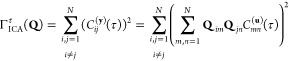
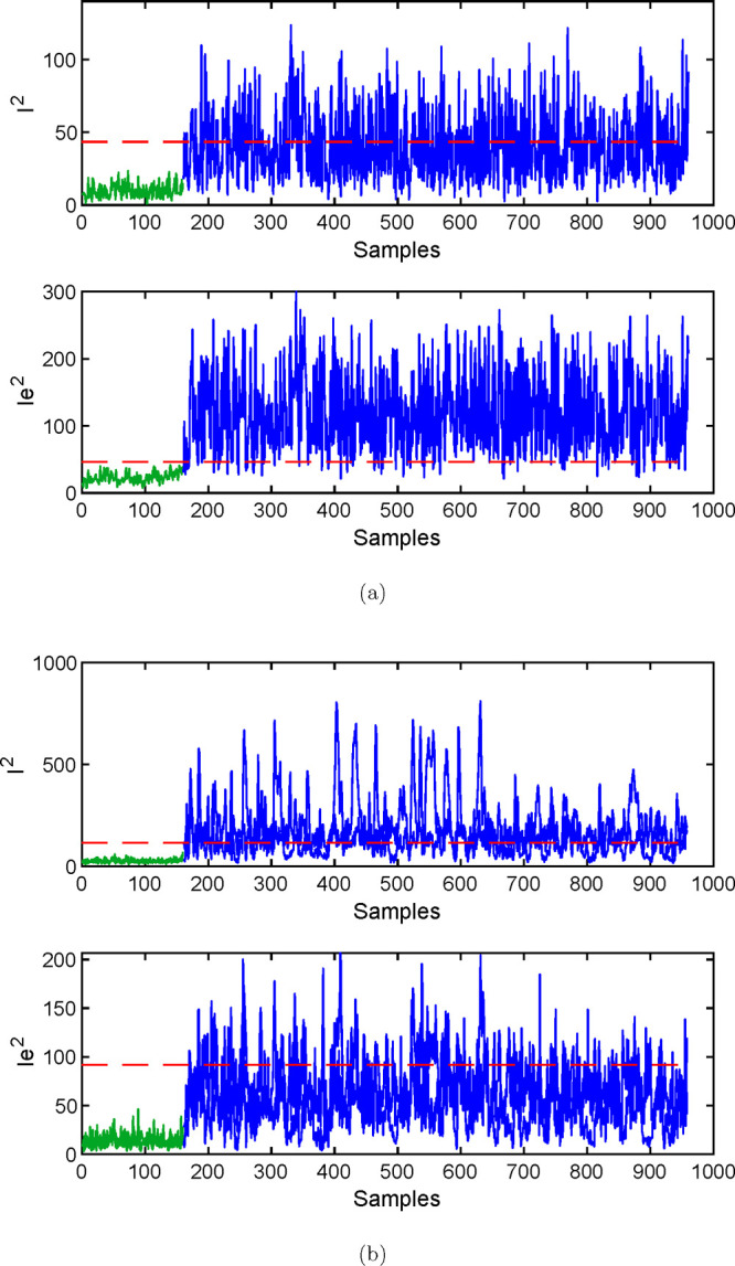
The monitoring results of ICA and dynamic ICA on fault 11 are shown in Figure 8, and the monitoring results of ISFA on fault 11 are shown in Figure 9. The FDRs of I2 and Ie2 in ICA are 45.12% and 72.12%, respectively. The FDR of I2 is lower than that of Ie2, and the process monitoring statistics of the fault samples fluctuate rapidly and repeatedly near the control limit. This shows that the information of fault 11 is mainly contained in the residual subspace of the ICA. The FDRs of I2 and Ie2 in dICA are 55% and 16.88%, respectively. The FDRs of the two process monitoring statistics are lower than that of ICA. This is because after dICA expands the dimensions of the data, it causes redundancy of information, which makes the effective information contained in the data less and ultimately leads to low detection results. The FDR of I2 in ISFA is 81.88%, which is significantly better than those of ICA and dICA. This shows that the fault information of fault 11 is mainly contained in the dominating subspace of ISFA, and ISFA has a stronger ability to extract appropriate LVs for the TE process.
Figure 8.

Monitoring results of the TE process for fault 11 using (a) ICA and (b) dICA.
Figure 9.

Monitoring results of the TE process for fault 11 using ISFA.
Fault 19 is an unknown fault; the monitoring results of ICA and dynamic ICA on fault 19 are shown in Figure 10, and the monitoring results of ISFA on fault 19 are shown in Figure 11. The process monitoring statistic Ie2 in ICA and I2 and Ie2 in ISFA can distinguish between normal data samples and fault data samples well. The FDRs of other process monitoring statistics are very low, and the values of process monitoring statistics fluctuate repeatedly around the control limit. The FDRs of I2 and Ie2 in ISFA are is 92.75% and 79.75%, respectively. The comprehensive FDRs of ISFA are higher than that of I2 in ICA, which is 90.38%. The FDRs of I2 and Ie2 in ISFA show that most of the fault information is contained in the dominating subspace of ISFA. It is further proved that when the number of LVs extracted is the same, ISFA can extract LVs that contain more process information and the extracted LVs can better describe the characteristics of the process.
Figure 10.
Monitoring results of the TE process for fault 19 using (a) ICA and (b) dICA.
Figure 11.

Monitoring results of the TE process for fault 19 using ISFA.
The average FARs of the three methods for 21 types of faults in the TE process are shown in Table 3. Compared with ICA, the FAR of the monitoring statistic I2 of our proposed method is increased by 5.98%, and the FDR is increased by 15.39%. The FAR of the monitoring statistic Ie2 of our proposed method is increased by 0.30%, and the FDR is decreased by 2.76%. On the monitoring statistic Ie2, the method we proposed failed to achieve better monitoring results than ICA. According to our analysis, there may be two reasons, which follow. On the one hand, the TE process data may not have the complex nonlinearities considered by our proposed method. This can be proved from the results of the numerical example. The performance of our proposed method has been greatly improved in numerical example. On the other hand, the feature extraction ability of our proposed method is stronger than that of ICA. Therefore, most of the useful process information is extracted into the dominating subspace, and the residual subspace contains less process information. Therefore, for the monitoring statistic Ie2, the performance is slightly worse than that of ICA. Compared with dynamic ICA, the FAR of the monitoring statistic I2 of our proposed method is increased by 5.98%, and the FDR is increased by 9.80%. The FAR of the monitoring statistic Ie2 of our proposed method is increased by 1.82%, and the FDR is increased by 22.50%. Although FARs have increased compared with dICA, considering the two indicators of FARs and FDRs, our proposed method outperforms dICA in the TE process.
Table 3. False Alarm Rates (%) of Each Method for TE Process.
| method | monitoring statistics | false alarm rate (%) |
|---|---|---|
| ICA | I2 | 0 |
| Ie2 | 1.52 | |
| dICA | I2 | 0 |
| Ie2 | 0 | |
| ISFA | I2 | 5.98 |
| Ie2 | 1.82 |
The performance of ISFA for process monitoring is significantly better than those of ICA and dICA. In addition, even for faults 3, 9, and 15, the FDRs of ISFA has increased by 10% compared to those of ICA and dICA.
Acknowledgments
This work was supported by the NSFC [Grant Nos. 61703158, 61933013, U1934221, 61733015, and 61733009]; the Huzhou Municipal Natural Science Foundation of China [Grant No. 2021YZ03]; the Zhejiang Province Key Laboratory of Smart Management & Application of Modern Agricultural Resources [Grant No. 2020E10017]; and the Postgraduate Scientific Research and Innovation Projects of Huzhou University [Grant No. 2020KYCX27].
The authors declare no competing financial interest.
References
- Joe Qin S. Statistical process monitoring: basics and beyond. Journal of Chemometrics: A Journal of the Chemometrics Society 2003, 17, 480–502. 10.1002/cem.800. [DOI] [Google Scholar]
- Qin S. J. Survey on data-driven industrial process monitoring and diagnosis. Annual reviews in control 2012, 36, 220–234. 10.1016/j.arcontrol.2012.09.004. [DOI] [Google Scholar]
- MacGregor J.; Cinar A. Monitoring, fault diagnosis, fault-tolerant control and optimization: Data driven methods. Comput. Chem. Eng. 2012, 47, 111–120. 10.1016/j.compchemeng.2012.06.017. [DOI] [Google Scholar]
- Jackson J. E.; Mudholkar G. S. Control procedures for residuals associated with principal component analysis. Technometrics 1979, 21, 341–349. 10.1080/00401706.1979.10489779. [DOI] [Google Scholar]
- Qin S. J.; Zheng Y. Quality-relevant and process-relevant fault monitoring with concurrent projection to latent structures. AIChE J. 2013, 59, 496–504. 10.1002/aic.13959. [DOI] [Google Scholar]
- Ku W.; Storer R. H.; Georgakis C. Disturbance detection and isolation by dynamic principal component analysis. Chemometrics and intelligent laboratory systems 1995, 30, 179–196. 10.1016/0169-7439(95)00076-3. [DOI] [Google Scholar]
- Hyvärinen A.; Oja E. Independent component analysis: algorithms and applications. Neural networks 2000, 13, 411–430. 10.1016/S0893-6080(00)00026-5. [DOI] [PubMed] [Google Scholar]
- Jutten C.; Karhunen J.. Advances in nonlinear blind source separation. Proceedings of the 4th International Symposium on Independent Component Analysis and Blind Signal Separation (ICA2003), Apr. 1–4, 2003, Nara, Japan; ICA2003, 2003; pp 245–256.
- Wiskott L.; Sejnowski T. J. Slow feature analysis: Unsupervised learning of invariances. Neural computation 2002, 14, 715–770. 10.1162/089976602317318938. [DOI] [PubMed] [Google Scholar]
- Wu C.; Zhang L.; Du B. Kernel slow feature analysis for scene change detection. IEEE Trans Geosci Remote Sens 2017, 55, 2367–2384. 10.1109/TGRS.2016.2642125. [DOI] [Google Scholar]
- Zhang Z.; Tao D. Slow feature analysis for human action recognition. IEEE Trans. Pattern Anal. Mach. Intell. 2012, 34, 436–450. 10.1109/TPAMI.2011.157. [DOI] [PubMed] [Google Scholar]
- Turner R.; Sahani M. A maximum-likelihood interpretation for slow feature analysis. Neural computation 2007, 19, 1022–1038. 10.1162/neco.2007.19.4.1022. [DOI] [PubMed] [Google Scholar]
- Zheng J.; Zhao C. Online monitoring of performance variations and process dynamic anomalies with performance-relevant full decomposition of slow feature analysis. J. Process Control 2019, 80, 89–102. 10.1016/j.jprocont.2019.05.004. [DOI] [Google Scholar]
- Zheng H.; Yan X. Extracting dissimilarity of slow feature analysis between normal and different faults for monitoring process status and fault diagnosis. J. Chem. Eng. Jpn. 2019, 52, 283–292. 10.1252/jcej.18we079. [DOI] [Google Scholar]
- Zheng H.; Jiang Q.; Yan X. Quality-relevant dynamic process monitoring based on mutual information multiblock slow feature analysis. J. Chemom 2019, 33, e3110 10.1002/cem.3110. [DOI] [Google Scholar]
- Zhao C.; Huang B. A full-condition monitoring method for nonstationary dynamic chemical processes with cointegration and slow feature analysis. AIChE J. 2018, 64, 1662–1681. 10.1002/aic.16048. [DOI] [Google Scholar]
- Zhang H.; Tian X.; Deng X. Batch process monitoring based on multiway global preserving kernel slow feature analysis. IEEE Access 2017, 5, 2696–2710. 10.1109/ACCESS.2017.2672780. [DOI] [Google Scholar]
- Yan S.; Jiang Q.; Zheng H.; Yan X. Quality-relevant dynamic process monitoring based on dynamic total slow feature regression model. Measurement Science and Technology 2020, 31, 075102. 10.1088/1361-6501/ab7bbd. [DOI] [Google Scholar]
- Shang C.; Huang B.; Yang F.; Huang D. Probabilistic slow feature analysis-based representation learning from massive process data for soft sensor modeling. AIChE J. 2015, 61, 4126–4139. 10.1002/aic.14937. [DOI] [Google Scholar]
- Qin Y.; Zhao C. Comprehensive process decomposition for closed-loop process monitoring with quality-relevant slow feature analysis. J. Process Control 2019, 77, 141–154. 10.1016/j.jprocont.2019.04.001. [DOI] [Google Scholar]
- Huang J.; Ersoy O. K.; Yan X. Slow feature analysis based on online feature reordering and feature selection for dynamic chemical process monitoring. Chemom Intell Lab Syst 2017, 169, 1–11. 10.1016/j.chemolab.2017.07.013. [DOI] [Google Scholar]
- Corrigan J.; Zhang J. Integrating dynamic slow feature analysis with neural networks for enhancing soft sensor performance. Comput. Chem. Eng. 2020, 139, 106842. 10.1016/j.compchemeng.2020.106842. [DOI] [Google Scholar]
- Shang C.; Yang F.; Gao X.; Huang X.; Suykens J. A.; Huang D. Concurrent monitoring of operating condition deviations and process dynamics anomalies with slow feature analysis. AIChE J. 2015, 61, 3666–3682. 10.1002/aic.14888. [DOI] [Google Scholar]
- Shang C.; Huang B.; Yang F.; Huang D. Slow feature analysis for monitoring and diagnosis of control performance. J. Process Control 2016, 39, 21–34. 10.1016/j.jprocont.2015.12.004. [DOI] [Google Scholar]
- Shang C.; Yang F.; Huang B.; Huang D. Recursive slow feature analysis for adaptive monitoring of industrial processes. IEEE Transactions on Industrial Electronics 2018, 65, 8895–8905. 10.1109/TIE.2018.2811358. [DOI] [Google Scholar]
- Zhang S.; Zhao C. Slow-feature-analysis-based batch process monitoring with comprehensive interpretation of operation condition deviation and dynamic anomaly. IEEE Transactions on Industrial Electronics 2019, 66, 3773–3783. 10.1109/TIE.2018.2853603. [DOI] [Google Scholar]
- Zhao C.; Chen J.; Jing H. Condition-Driven Data Analytics and Monitoring for Wide-Range Nonstationary and Transient Continuous Processes. IEEE Transactions on Automation Science and Engineering 2021, 18, 1563–1574. 10.1109/TASE.2020.3010536. [DOI] [Google Scholar]
- Blaschke T.; Wiskott L. Independent slow feature analysis and nonlinear blind source separation. International Conference on Independent Component Analysis and Signal Separation 2004, 3195, 742–749. 10.1007/978-3-540-30110-3_94. [DOI] [Google Scholar]
- Sprekeler H.; Wiskott L.. Understanding slow feature analysis: A mathematical framework. Available at SSRN 3076122 SSRN J. 2008,. 10.2139/ssrn.3076122 [DOI] [Google Scholar]
- Blaschke T.; Zito T.; Wiskott L. Independent slow feature analysis and nonlinear blind source separation. Neural computation 2007, 19, 994–1021. 10.1162/neco.2007.19.4.994. [DOI] [Google Scholar]
- Molgedey L.; Schuster H. G. Separation of a mixture of independent signals using time delayed correlations. Physical review letters 1994, 72, 3634. 10.1103/PhysRevLett.72.3634. [DOI] [PubMed] [Google Scholar]
- Ziehe A.; Müller K.-R. TDSEP—an efficient algorithm for blind separation using time structure. International Conference on Artificial Neural Networks 1998, 675–680. 10.1007/978-1-4471-1599-1_103. [DOI] [Google Scholar]
- Blaschke T.; Berkes P.; Wiskott L. What is the relation between slow feature analysis and independent component analysis?. Neural computation 2006, 18, 2495–2508. 10.1162/neco.2006.18.10.2495. [DOI] [PubMed] [Google Scholar]
- Blaschke T.; Wiskott L. CuBICA: Independent component analysis by simultaneous third- and fourth-order cumulant diagonalization. IEEE Trans. Signal Process. 2004, 52, 1250–1256. 10.1109/TSP.2004.826173. [DOI] [Google Scholar]
- Lee J.-M.; Yoo C.; Lee I.-B. Statistical monitoring of dynamic processes based on dynamic independent component analysis. Chem. Eng. Sci. 2004, 59, 2995–3006. 10.1016/j.ces.2004.04.031. [DOI] [Google Scholar]
- MacGregor J. F.; Jaeckle C.; Kiparissides C.; Koutoudi M. Process monitoring and diagnosis by multiblock PLS methods. AIChE J. 1994, 40, 826–838. 10.1002/aic.690400509. [DOI] [Google Scholar]
- Hong H.; Jiang C.; Peng X.; Zhong W. Concurrent monitoring strategy for static and dynamic deviations based on selective ensemble learning using slow feature analysis. Ind. Eng. Chem. Res. 2020, 59, 4620–4635. 10.1021/acs.iecr.9b05547. [DOI] [Google Scholar]
- Chen Q.; Wynne R.; Goulding P.; Sandoz D. The application of principal component analysis and kernel density estimation to enhance process monitoring. Control Engineering Practice 2000, 8, 531–543. 10.1016/S0967-0661(99)00191-4. [DOI] [Google Scholar]
- Kano M.; Hasebe S.; Hashimoto I.; Ohno H. Evolution of multivariate statistical process control: application of independent component analysis and external analysis. Comput. Chem. Eng. 2004, 28, 1157–1166. 10.1016/j.compchemeng.2003.09.011. [DOI] [Google Scholar]
- Silverman B. W.Density estimation for statistics and data analysis; Routledge, 2018. 10.1201/9781315140919. [DOI] [Google Scholar]
- Harmeling S.; Ziehe A.; Kawanabe M.; Müller K.-R. Kernel-based nonlinear blind source separation. Neural Computation 2003, 15, 1089–1124. 10.1162/089976603765202677. [DOI] [Google Scholar]
- Downs J. J.; Vogel E. F. A plant-wide industrial process control problem. Comput. Chem. Eng. 1993, 17, 245–255. 10.1016/0098-1354(93)80018-I. [DOI] [Google Scholar]
- Chiang L. H.; Russell E. L.; Braatz R. D.. Fault detection and diagnosis in industrial systems; Springer Science & Business Media, 2000. [Google Scholar]
- Yin S.; Ding S. X.; Haghani A.; Hao H.; Zhang P. A comparison study of basic data-driven fault diagnosis and process monitoring methods on the benchmark Tennessee Eastman process. J. Process Control 2012, 22, 1567–1581. 10.1016/j.jprocont.2012.06.009. [DOI] [Google Scholar]
- Lyman P. R.; Georgakis C. Plant-wide control of the Tennessee Eastman problem. Comput. Chem. Eng. 1995, 19, 321–331. 10.1016/0098-1354(94)00057-U. [DOI] [Google Scholar]
- Cai L.; Thornhill N. F.; Pal B. C. Multivariate Detection of Power System Disturbances Based on Fourth Order Moment and Singular Value Decomposition. IEEE Transactions on Power Systems 2017, 32, 4289–4297. 10.1109/TPWRS.2016.2633321. [DOI] [Google Scholar]