

Abstract
Adaptive optics (AO) is a technique that corrects for optical aberrations. It was originally proposed to correct for the blurring effect of atmospheric turbulence on images in ground-based telescopes and was instrumental in the work that resulted in the Nobel prize-winning discovery of a supermassive compact object at the centre of our galaxy. When AO is used to correct for the eye’s imperfect optics, retinal changes at the cellular level can be detected, allowing us to study the operation of the visual system and to assess ocular health in the microscopic domain. By correcting for sample-induced blur in microscopy, AO has pushed the boundaries of imaging in thick tissue specimens, such as when observing neuronal processes in the brain. In this primer, we focus on the application of AO for high-resolution imaging in astronomy, vision science and microscopy. We begin with an overview of the general principles of AO and its main components, which include methods to measure the aberrations, devices for aberration correction, and how these components are linked in operation. We present results and applications from each field along with reproducibility considerations and limitations. Finally, we discuss future directions.
High-resolution optical imaging relies upon the high-fidelity focusing of light. Light can be described in terms of its optical field, and thus its properties are parameterized for a given wavelength at each point in space and time in terms of amplitude, phase and polarization. However, these fields can be perturbed (in amplitude, phase and polarization) as they propagate through optical systems and other media, and the performance of the imaging systems can be highly sensitive to those perturbations. For instance, astronomical image quality is limited by atmospheric turbulence; microscopes produce blurred images when samples have a non-uniform refractive index distribution; and ophthalmoscopes that image the back of the eye are detrimentally affected by the eye’s imperfect optics. Adaptive optics (AO) is an ensemble of electro-optical and computational methods that aim to recover the optimal performance of an optical system1–6. This has brought benefits to a range of applications. For example, by integrating AO in their telescopes, astronomers have been able to expand the observation of celestial bodies7. Implemented into microscopes, AO has enabled neuroscientists to monitor the activity of neurons embedded deep inside the living mammalian brain8,9. And integrated into ophthalmoscopes, it has enabled vision scientists and ophthalmologists to visualize, quantify and track in situ the many different types of cell that compose the retina, offering significant clinical potential10–14.
Optical field.
Describes the distribution of light as an electrical field across space and time in terms of amplitude, phase, frequency and polarization.
There are many imaging applications in which AO has a significant impact, and the above list is far from exhaustive. Compensation through modulation of the optical field is the fundamental working principle through which AO alleviates the effect of optical aberrations15. Most commonly, we consider aberrations as variations in phase of the optical field. Such phase variations are equivalent to changes in the wavefront shape16. In general, aberrations can be understood as deformations of the light’s wavefront from its perfect form — planar for a collimated beam or spherical for a focusing beam — that produces the sharpest image1,2. Wavefront aberrations, such as those caused by refractive index variations in biological tissue or air motion, can be rectified by locally modulating the phase of the light such that the effects of the aberrations and the applied modulation cancel out16. In other words, the optimal wavefront shape is recovered by introducing a modulated wavefront with its phase conjugate to the problematic aberrations. This process of correction is one of the two essential components shared by all AO methods. The other process consists of evaluating or sensing the aberrations, to determine the optimal phase compensation. Instead of using a dedicated sensor, the image can also be used to determine the appropriate correction. There is wide diversity in approaches to realize both sensing and correction1–4. In addition, implementation requirements can vary widely between fields in which AO is used, making it challenging to translate key concepts and methods across applications. However, connecting these concepts is worthwhile, as fundamental advances in AO originate from all these application areas, and developers can benefit from important advances in separate fields.
Compensation.
Reduction of an effect by modulation of the optical field through introducing the opposite effect.
Focusing.
All rays being brought to meet at one point.
In this Primer, we aim to provide a unified perspective on AO for imaging applications by highlighting commonalities, and differences where necessary, in experimentation between fields. We present results from astronomy, vision science and microscopy to illustrate the potential of AO for improving images in a range of imaging modalities and then discuss how the improvements afforded by AO facilitate and enable new scientific discoveries in diverse applications. For this purpose, we select exemplar results and applications and discuss them in varying levels of detail to reflect intrinsic properties of AO in different fields and modalities. We give information about external resources to ease the adoption of AO and support reproducibility. Finally, we consider current limitations of AO methods before we present an outlook on anticipated technology development.
Experimentation
Different application fields using AO for imaging have their particular technical requirements and AO implementations. However, there are many underpinning concepts that are common to all applications. In this section, we review the fundamental principles and methods of implementing AO and how and why this varies for different fields.
Generic AO system for imaging
The image quality of an optical system is typically characterized by its point spread function (PSF). The PSF describes how the image of a point is blurred when light passes through the optical system. The degree of blurring depends upon the shape of the wavefront. FIGURE 1a illustrates the concept of a wavefront and its distortion. The propagation of light is represented conceptually by multiple adjacent waves. The shape of the wavefront, W, is found by joining up the peaks of each wave, which is where the light has the same phase. Note that the ray directions are locally orthogonal to the wavefront. Initially the wavefront is planar. When the light reaches an object that has a non-uniform refractive index distribution, the different waves travel at different speeds, causing them to be delayed with respect to each other. In the example shown, the central wave travels through a medium with a relatively high refractive index, which causes the light in that region to travel more slowly. The consequence of this is that the outgoing waves are now out of phase owing to the difference in optical path length. The PSF of an imaging system is directly related on the shape of the wavefront in the pupil plane of the system, where the limiting optical aperture is typically placed. Although the above example is two-dimensional for simplicity, it should be kept in mind that a wavefront is a surface in a three-dimensional space. For an aberration-free system, the wavefront is planar in the pupil plane as the light is typically collimated. This results in a spherical wave when the light is focusing to form the image. The resulting PSF is diffraction-limited, as shown in FIG. 1b. The diffraction-limited PSF is the smallest obtainable image of a point and sets the resolution limit of an imaging system (unless super-resolution techniques are employed, such as structured illumination)17. According to the Rayleigh resolution criterion, for two point objects to be resolved, the maximum intensity of the PSF of one object must lie on or further from the first minimum of the PSF of the other. The narrower the PSF, the closer the two objects can be in order to be resolved. This resolution, R, is set by the diffraction limit and given by
| (1) |
where λ is the wavelength, f is the focal length and d is the pupil diameter.
Fig. 1 |. The nature and effect of wavefront aberrations and how they are corrected.
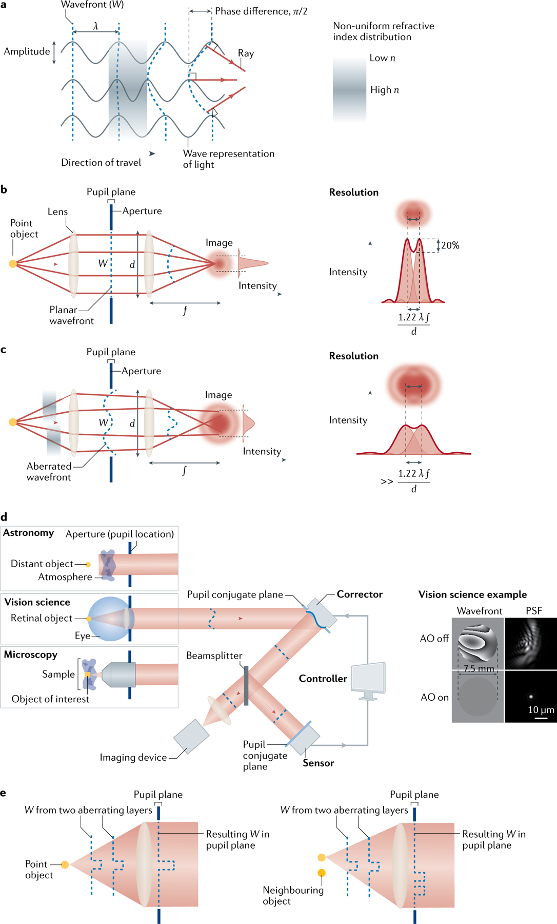
a | The relationship between the wavefront and how it is affected by changes in optical path. The central light wave is slowed down relative to the outer light waves owing to it passing through a medium with a higher refractive index in that region. The result is the wavefront becoming distorted. b | In an aberration-free system, the wavefront is planar in the pupil plane and resolution is diffraction-limited. c | When aberrations are present, the pupil plane wavefront is distorted and resolution decreases. The thick red lines outlining the point spread functions (PSFs) represent the normalized sum of the individual PSFs. d | General adaptive optics (AO) system. The corrector shown here is a deformable mirror, but could in principle be another device. Wavefront aberrations at the eye’s pupil and corresponding PSFs at the retina for a typical eye with and without perfect AO. Wavefront maps are shown with a modulo-2π greyscale. e | How multiple aberration layers affect the pupil wavefront for different points in the imaged field.
Optical path length.
The length of the path followed by a light ray multiplied by the refractive index of the medium.
Pupil plane.
Aperture stop location.
Collimated.
All rays are parallel to each other.
Diffraction-limited.
There are no aberrations present in the focus. The minimum focal diameter is limited by diffraction owing to the wave nature of light.
Focal length.
The distance between a lens and where the rays meet the optical axis for incoming collimated light.
When aberrations are present, for example, owing to refractive index inhomogeneities in the medium through which the light must pass, as in the case of microscopy and astronomy, or the optical components having a non-ideal shape, as in the case of vision science, the wavefront is no longer described by a plane or spherical wave, as shown in FIG. 1c. Consequently, the maximum intensity of the PSF is reduced and the width of the PSF is increased, resulting in reduced image resolution and contrast, as shown by comparing the right-hand sides of FIG. 1b,c. The goal of AO is to introduce a distortion that is equal in magnitude but opposite in sign to that of the aberrated wavefront, to correct for aberrations and achieve diffraction-limited image quality with maximal signal. This is achieved by changing the optical path length using deformable mirrors, for example. The magnitude of the wavefront distortion is typically specified in micrometres (μm). To achieve diffraction-limited resolution, which is equivalent to a Strehl ratio of 0.8 or above, AO must reduce this distortion to less than λ/14. Note that amplitude variations that result in intensity variations, whereby the amplitude is denoted by the peak-to-valley of the wave as shown in FIG. 1a, are typically neglected. This is primarily owing to phase distortions having a more pronounced effect on the imaging properties. In addition, intensity correction with current devices would involve introducing losses. Similarly, distortions of the polarization state are also often neglected despite polarization control gaining interest in microscopy, as it is important in some imaging modalities18,19.
Strehl ratio.
The ratio of the intensity of the peak of the aberrated point spread function (PSF) to that of the diffraction-limited PSF.
A general AO imaging system is shown in FIG. 1d. It consists of three main components: a sensor to measure the aberrations, a corrector to compensate the aberrations and a controller that calculates the required signals sent to the corrector based on the sensor measurements. The corrector and sensor are typically conjugate to the pupil plane of the imaging system, which means that the pupil is imaged on to the corrector and sensor. In the case of microscopy, the pupil is the aperture of the objective lens that transfers light to and from the specimen. For vision science, it is the eye’s pupil and for astronomy, it is the telescope aperture. Conjugation of the corrector, sensor and system pupil is achieved via pairs of lenses or curved mirrors, called relay telescopes, that reimage each one on to the next20–22. AO systems are typically designed using commercial optical ray tracing software such as Zemax and constructed from a myriad of mostly high-end stock lenses and mirrors. In some AO systems, there is no dedicated wavefront sensor and the quality of the image is used to control the corrector. Although this method has some advantages such as reduced system complexity, it is also slow and is not suitable for situations in which the aberrations are rapidly evolving. Consequently, this technique is mainly confined to microscopy. Note that the system shown in FIG. 1d is a generic AO imaging system. Different fields have various different imaging systems with specific AO implementation.
Across all fields, the aberrations that are induced originate from multiple layers. In astronomy the turbulence varies with altitude, while in the eye aberrations are introduced mostly by the surfaces of the crystalline lens and cornea. For microscopy, there can be a volume of inhomogeneous tissue in front of the object of interest. This means that the shape of the wavefront varies depending upon the location of the object of interest as shown in Fig. 1e. The most straightforward method for aberration compensation is to update a single corrector accordingly. Use of a single corrector is referred to as single-conjugate AO (SCAO) and is the most widely used implementation of AO. A less commonly employed method is to use multiple correctors, in which each corrector is conjugate to a different layer or depth. This is referred to as multiconjugate AO (MCAO)23–25. This adds significant cost and complexity to an AO system.
The area over which the aberrations can be considered invariant is referred to as the isoplanatic patch. Typical values for the isoplanatic patch for astronomy are 1.5 arcsec to 2 arcsec at a wavelength of 0.5 μm, varying with seeing and turbulence layer heights, and scaling with wavelength to the 6/5 power3,26. For vision science it is approximately 1°, or 300 μm at the retina27. In the case of microscopy, the patch size ranges from hundreds of microns, in mouse brain for example8,28,29, to a few microns, such as inside tissue with high curvature or complexity, for example, zebrafish larvae30 or Caenorhabditis elegans29,31. Although a single corrector is commonly placed in a pupil conjugate plane, it can be more advantageous to place a single corrector conjugate to the layer introducing the most significant aberrations. This can widen the field of view over which sharp images are obtained. This is referred to as ground-layer AO in astronomy and sample-conjugate AO in microscopy32.
In all cases, the temporal dynamics of the perturbations must be considered as this has implications for the way in which AO is implemented. Although some perturbations are relatively stable, often the case in microscopy applications, perturbations due to dynamic processes in the eye can vary significantly, with perturbations due to atmospheric turbulence evolving even more quickly. We note that in astronomy there is a distinction between active optics and AO. Active optics involves changing the shape of the telescope mirrors to account for environmental factors and to align and collimate the telescope; its role is not to correct aberrations due to turbulence and is much slower than AO33. There is no such semantic distinction in vision science and microscopy.
Aberration characteristics
When implementing AO, it is important to consider the properties of the aberrations to be corrected. This includes what type of aberrations are present and how rapidly the wavefront changes shape over time. The shape of the wavefront, W, can be considered to consist of a sum of shapes or modes. It is common for these modes to be expressed in terms of Zernike polynomials34:
| (2) |
where ρ is the normalized pupil radius ranging from zero to one, θ is the angle around the optical axis, and is the coefficient (or magnitude) of the Zernike polynomial with the azimuthal frequency m and radial order n. We note that there are certain constraints on the allowable values of m and n. Each polynomial describes the shape of the wavefront for a given aberration (or mode). Each of these modes is shown in FIG. 2. Several Zernike modes correspond closely to aberrations used in classical optics such as astigmatism and coma. An advantage of Zernike polynomials is that they are orthogonal, that is, they have convenient mathematical properties that permit us to consider them as having independent effects on the optical system. There are slight variations on the definition of Zernike polynomials, such as whether the angles are measured clockwise or anticlockwise. FIGURE 2 shows the Zernike aberrations as defined by the Noll convention35,36, which are typically used in astronomy and microscopy. In vision science, the OSA ANSI convention is commonly used because the way in which the angle is measured matches the way it is defined when determining a patient’s spectacle or contact lens prescription37. The piston mode, which is a constant phase offset and can be seen at the top of FIG. 2, is not considered when correcting the wavefront as it does not affect the image because it merely represents translation of the wavefront along the optical axis. Tip and tilt represent a shift in the position of the image and so are not usually corrected for in microscopy with stationary samples. In vision science, even when the eye is fixated on a static object, miniature eye movements cause the retina to rapidly move around. In scanning imaging systems for the eye, in which the image is built up line by line, this can cause image distortion. Tip and tilt changes due to atmospheric turbulence also cause image blur that needs to be corrected. Note that in the literature, aberration modes are often broadly categorized as being of lower order or higher order. The definition of lower order and higher order varies between fields. Higher order is typically defined as modes with a radial order above three for astronomy, above two for vision science and above four for microscopy.
Fig. 2 |. Modal representation of aberrations using Zernike polynomials according to the Noll notation35.
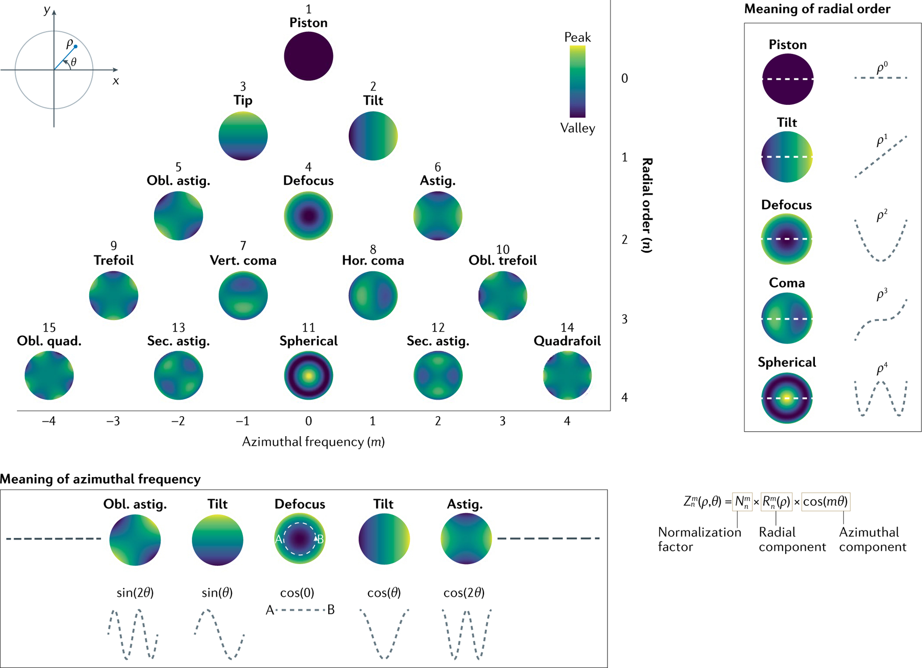
The polynomials are organized according to their radial order n and azimuthal frequency m. The radial component describes how the polynomial varies with the radius ρ. For example, a mode with a radial order of two means that the polynomial describing the mode has a mathematical term where the highest power is two, that is, it has a ρ2 term. The azimuthal frequency describes how the polynomial varies with angle θ. The positive numbers represent a cosinusoidal variation, with negative numbers representing sinusoidal variation. For example, a value of 2 means that the polynomial varies with cos(2θ). Astig., astigmatism; Hor., horizontal; Obl., oblique; Sec., secondary; Vert., vertical. Adapted with permission from REF.36, Zenodo. CC BY NC-ND 4.0.
Noll convention.
Mathematical description of aberrated wavefront shapes as proposed by Noll.
A summary of the properties of the aberrations for each field are shown in TABLE 1. In astronomy and vision science, there are statistical models of the aberrations38–40. These mathematical models generate the sort of aberrations that are likely to occur based on experimental parameters such as pupil diameter of the eye or the telescope41. In astronomy, the number of Zernike modes corrected varies from facility to facility and depends on the type of AO implementation, but can vary from the order of one hundred to several thousand, equivalent to radial orders from 15 to ~70. The higher the radial order, the lower the magnitude of the aberration35. The peak-to-valley wavefront amplitude is typically 1–3 μm root mean square (rms). The dominant source of temporal evolution is wind-driven motion of the atmosphere42. Depending on telescope diameter and wind speed, aberrations can vary with frequencies up to 100 Hz (REF.43). The variation in aberration magnitude with temporal frequency follows a power law with an exponent of −17/3 (REFS44,45). In vision science, the aberrations increase with pupil size and typically the higher the Zernike radial order, the lower the magnitude of the aberration46. The pupil of the eye is often dilated when imaging the retina to increase resolution. For a 7.5 mm pupil, achieving diffraction-limited imaging in 95% of the population requires correction of the Zernike radial orders from two to ten40. The peak-to-valley of the wavefront is around 11 μm, but is much higher if the individual requires a spectacle prescription (radial order two). These aberrations also temporally vary, most likely owing to dynamics in the optics of the eye caused by the heartbeat, tear film instabilities and movement of the eye. The power law exponent of these fluctuations is about −1.3 (REFS47,48). Today’s ophthalmic AO systems are generally designed to handle dynamic aberrations up to a couple of Hertz, but a recent study that included many more individuals suggests that correcting fluctuations varying at higher frequencies may be necessary to achieve diffraction-limited performance in most eyes49.
Table 1|.
Comparison of aberration characteristics and their correction across fields
| Field | Aberrations | Sensors | Correctors | Control |
|---|---|---|---|---|
|
| ||||
| Astronomy | Main source is wind-driven motion of the atmosphere Wavefront variance decays with Zernike radial order following a power law with exponent −11/3 Temporal PSD varies with f−17/3 Peak-to-valley wavefront is 1–3 μm rms Isoplanatic patch size is 1.5–2 arcsec at 500 nm Correcting between 15 and 70 Zernike radial orders is typical |
SH sensor most widely used SH lenslets to actuators ratio ~1:1 Pyramid sensors increasingly used |
Continuous surface DMs most widely used Typical number of DM actuators: 100s–1,000s |
Closed-loop systems by far the most common Closed-loop bandwidth of 50 Hz is typical Integral controller is most widely used |
|
| ||||
| Vision science | Main source is optical imperfections in the crystalline lens and cornea Wavefront variance decays exponentially with Zernike radial order in the range −1.1 to −1.8 Temporal PSD varies with f−1.3 – f−1.5 Peak-to-valley wavefront is 7–11 μm for a dilated pupil with no refractive error Isoplanatic patch size is about 300 μm Correcting 10 Zernike radial orders is typical for a dilated pupil |
SH sensor most widely used SH lenslets to actuators ratio 3:1–6:1 |
Continuous surface DMs most widely used Typical number of DM actuators <100 |
Closed-loop systems by far the most common Closed-loop bandwidth of <2 Hz is typical Integral controller is most widely used |
|
| ||||
| Microscopy | Main source is shape and refractive index inhomogeneity of cells and tissue Aberration magnitudes vary with sample Aberrations are mostly temporally static Peak-to-valley wavefront varies from submicrometre to several microns Isoplanatic patch size is several to 100s of microns Correcting between 7 and 11 Zernike radial orders is typical |
Indirect sensing and SH are both common SH lenslets to actuators ratio ~1:1 Indirect sensing employs both modal and zonal aberration representation |
Continuous DMs most widely used LCSLMs used in laser illumination paths Segmented DMs used for high-order scattering compensation Typical number of DM actuators <100 Typical number of SLM pixels 512 × 512 |
Open- and closed-loop systems are both common As aberrations are mostly static, closed-loop dynamics are determined by imaging speed |
DM, deformable mirror; f, frequency; LCSLM, liquid crystal spatial light modulator; PSD, power spectral density; rms, root mean square; SH, Shack–Hartmann.
Although the aberration characteristics of some microscopy samples have been shown to be similar to that of astronomy with regard to the decrease in magnitude of the Zernike aberrations with increasing radial order50, there are no comprehensive statistical models for microscopy owing to the vast range of specimen types for which AO might be used. Aberrations of samples with flat geometries and a homogeneous refractive index distribution are dominated by Zernike modes up to and including the fourth radial order, while samples with more complex shaped surfaces and/or heterogeneous refractive index distributions require correction of many aberration modes beyond these. Similarly, the magnitudes of aberrations in microscopy depend on the sample, and can vary from submicrometre to several microns. Even for microscopy of live specimens, sample-induced aberrations usually do not vary rapidly over time. Therefore, AO measurement and correction do not have to be carried out at high speed.
A useful descriptor to capture the severity of the aberrations in a system is the rms wavefront error. This is given by the square root of the sum of the squared coefficients. An aim of AO is to reduce this value to less than λ/14 to obtain diffraction-limited resolution. Although Zernike modes are commonly used, they are not the only — nor necessarily the best — representation for a particular application. Other analytically or empirically defined mode sets can also be used that represent a more efficient basis than Zernike modes. For example, for vision science see REFS40,51. Furthermore, when operating an AO system, it is often convenient to think of the wavefront as consisting of discrete non-overlapping zones, or segments, as opposed to a sum of superimposed modes. The choice of modes or zones often depends on the implementation of sensing and correction, which is discussed further in the relevant sections.
Aberration measurement
Aberrations can be measured most directly using a dedicated wavefront sensor, or they can be determined indirectly from the images. We refer to these two methods as direct sensing and indirect sensing, respectively. The indirect method is often referred to as sensorless AO as there is no dedicated wavefront sensor. Indirect methods are significantly slower than sensor-based methods at determining the magnitude of the aberrations present and the required correction. This is because they typically require collection of many images. Depending on the imaging speed, indirect methods can take seconds to minutes to determine the required correction in comparison with milliseconds for a dedicated wavefront sensor. As the aberrations in microscopy are mostly static, indirect methods are more suited to this field. Indirect methods have also been used to some extent in vision science — see for example, REF.52 — owing to the advantage of requiring no extra sensing hardware. However, for astronomy, in which the aberrations due to atmospheric turbulence evolve at high rates, the slow speed of indirect sensing would present a significant problem. A summary of the typical sensors used for each field and their properties is shown in TABLE 1.
Direct sensing.
The most widely used sensor to measure the aberrations across all fields in an AO system is the Shack–Hartmann (SH) sensor, as it can be quick, simple and effective16. The principle of operation is shown in FIG. 3a. It consists of an array of lenslets placed in a pupil conjugate plane and a camera at the focal plane of the lenslets53. For an aberration-free wavefront, a regular and evenly spaced array of spots is formed on the camera. For an aberrated wavefront, the location of each spot is shifted according to the local tilt (or slope) of the wavefront across that given lenslet as shown in FIG. 3b. Typically, a minimum of four camera pixels per spot is required to accurately determine the location of a spot. There are various algorithms for determining spot locations, with the centre of mass being one of the most frequently used54. Finding the centre of the spot using the centre of mass is often referred to as centroiding.
Fig. 3 |. Principles of the Shack–Hartmann wavefront sensor and pyramid wavefront sensor.
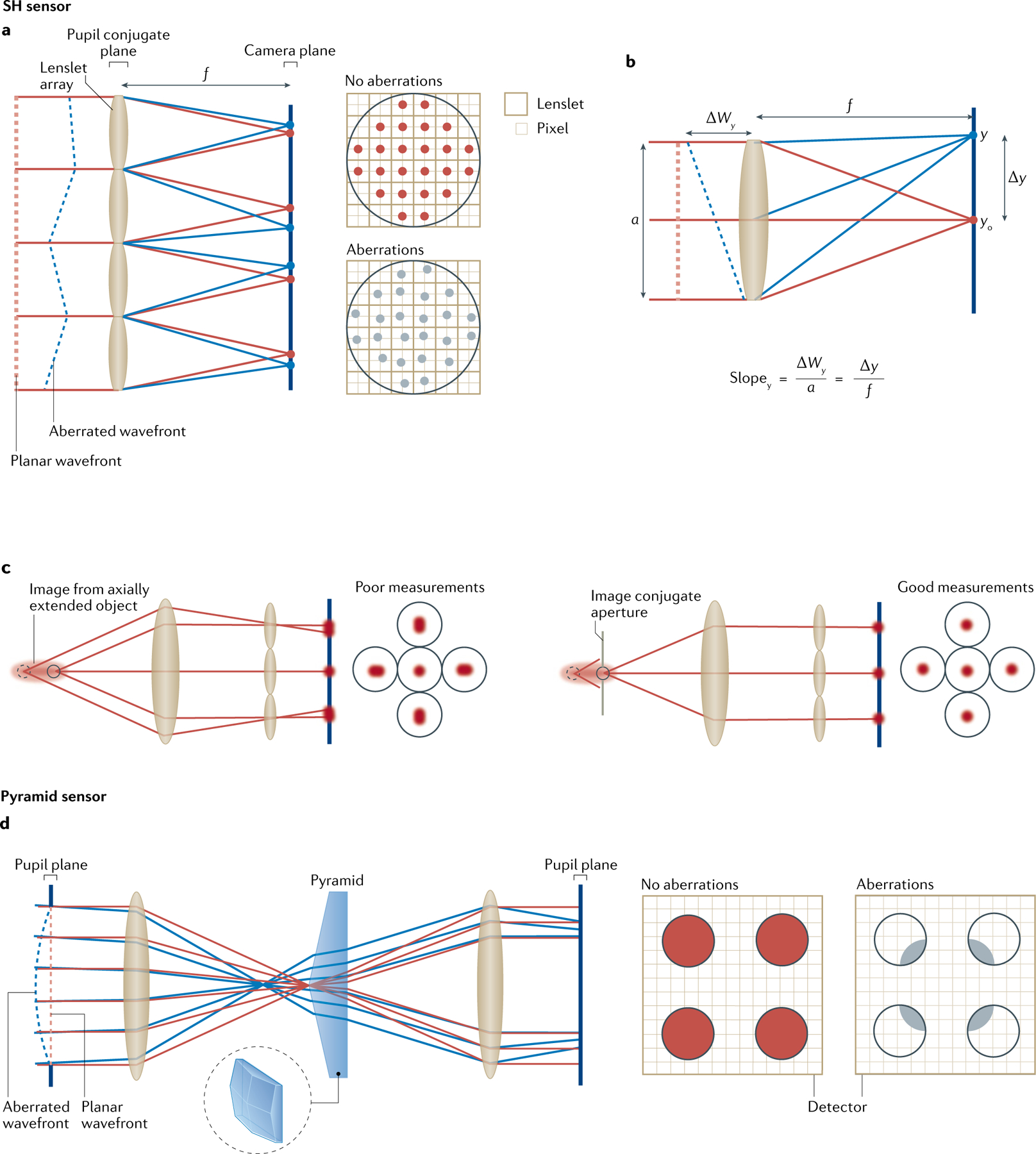
a | The Shack–Hartmann (SH) sensor consists of a lenslet array conjugate to the pupil plane and a camera placed at the focal plane of the array. For an aberration-free wavefront, a regularly spaced array of spots is formed on the camera. In the example shown there are four camera pixels behind each lenslet. b | Aberrations shift each spot according to the local wavefront slope, slopey (and slopex), across each lenslet. The magnitude of the wavefront, ΔWy (and ΔWx), across a lenslet of diameter a, is determined from the shift in the spot, Δy (and Δx), divided by the focal length, f. c | To obtain the slope using conventional SH algorithms, the light returning from the object must be point-like, that is, confined axially and laterally. Otherwise, the SH spots will be elongated, which can adversely affect the algorithm to determine their precise location. For light that is axially elongated, an image conjugate aperture can be used to alleviate these problems by reducing the amount of out-of-focus light reaching the sensor. d | Pyramid wavefront sensor. A four-faceted prism is placed at the focal plane and forms four images of the pupil. For an aberration-free or planar wavefront, four pupil images, with identical intensity distributions, are imaged on to the detector. Aberrations result in changes to the intensity distribution of each pupil image. An example for defocus is shown.
Lenslets.
Miniature lenses usually as part of an array.
Note that the traditional implementation of the SH sensor requires light returning from a point source to inform the sensor measurements. In microscopy, this could be light originating from a point object, for example, a fluorescent bead. In vision science the retina is typically illuminated with a point of light from an infrared (IR) light source. If the light informing the SH sensor is not confined axially and laterally the SH spots will become elongated. FIGURE 3c shows an example of spot elongation owing to an axially extended object where light is returning from multiple depths. This effect is more pronounced with higher numerical apertures and therefore occurs more in microscopy than in vision science55,56. When elongated spots are present, either an image conjugate aperture can be used (as shown in FIG. 3c57) or more advanced algorithms must be implemented. Spot elongation is inherent in astronomy when using laser guide stars (LGSs) to provide light to inform the wavefront sensing measurements. Some astronomical AO systems implement image-based SH wavefront sensing58, in which the image of the object of interest, such as the surface of the Sun, forms behind each lenslet, and the shift of each of these images determines the local slope of the wavefront. An advantage of this technique is that there is no need for an extra light source for the SH. This technique is starting to be adopted in microscopy59 but has yet to be used in vision science. In astronomy, multiple wavefront sensors can be used to reconstruct the turbulence based on measurements from multiple guide stars, even if a single corrector (SCAO) is to be used. Called tomographic AO60, this technique is used to calculate the shape of the corrector for aberration-free imaging of an object of interest within the field of view. Using the light of multiple guide stars is necessary because the light from a single guide star can take a very different path through the turbulence in comparison with the light from the object. Consequently, the aberration measurements from a single guide star may not be appropriate.
When using a deformable mirror as the corrector, astronomical and microscopy AO systems typically use a ratio of the total number of lenslets to the total number of actuators of around one, owing to limited light9,16. For vision science AO systems, where considerably more light is available for wavefront sensing, a minimum ratio of about two has been reported as optimal61, but a typical ratio in actual systems is between three and six. Once the ratio has been set, the focal length should be chosen to be the longest possible before the SH spots cross into regions behind neighbouring lenslets. This is to keep the highest sensitivity possible without exceeding the desired dynamic range. The longer the focal length the higher the sensitivity in detecting the movement of the spots, but if the focal length is too large, the spots will quickly cross into regions behind neighbouring lenslets and reduce the dynamic range. Consequently, there is a trade-off between sensitivity and dynamic range.
Actuators.
Elements that deform the mirror.
Dynamic range.
The range between the smallest and largest measurable values.
Although the SH is the most widely used sensor, there are several alternatives16. For instance, curvature and pyramid sensors are used in astronomy, with the curvature sensors being phased out and the pyramid sensors being increasingly used. FIGURE 3d shows the principle of operation of the pyramid wavefront sensor, which uses a different principle to encode phase variations into intensity measurements62. The tip of a four-faceted prism is placed at the image plane and the prism forms four images of the pupil. The aberrations present are determined from the relative intensity distributions of the pupil images. For a planar, that is, aberration-free wavefront, each pupil image is illuminated identically. When an aberration is present, for example, defocus, the light is refracted by the prism such that each pupil is illuminated differently. An advantage of this sensor in comparison with the SH is that the dynamic range and sensitivity can be adjusted independently63 and a wider range of aberration magnitudes, from low to high, can be measured accurately. The pyramid sensor has been demonstrated across fields63–65 but is not yet used as extensively as the SH sensor, perhaps owing to a later introduction in AO compared with the SH. In the future there may be other direct-sensing alternatives to the SH sensor such as diffusive plates, whereby the local wavefront slope is determined from the local shift in the resultant speckle pattern66. Another approach is to use machine learning to improve the sensor performance in heavy scattering, scintillation or when sensor spots are distorted or obscured66,67.
Indirect sensing.
Two main types of indirect sensing are modal and zonal. In the modal case, a continuous surface wavefront corrector is used, and the wavefront consists of the sum of aberration modes, as illustrated in FIG. 2. Individual aberration modes, such as Zernike modes, are applied sequentially to the wavefront corrector, and changes in the image are quantified using an image quality metric such as intensity or image sharpness1. FIGURE 4a shows a simple example in which coma is present. By applying different magnitudes of coma to the corrector and measuring the intensity in the image, a parabolic curve can be fitted to the data points to determine the optimum amount of coma that must be introduced to obtain a clear image. Other modes can be corrected in a similar way. Recent work has shown that wavelet decomposition of images provides a versatile way to define optimization metrics for indirect sensing68. There are several algorithms that have been used to determine the correction in modal schemes5,69.
Fig. 4 |. Indirect sensing schemes.
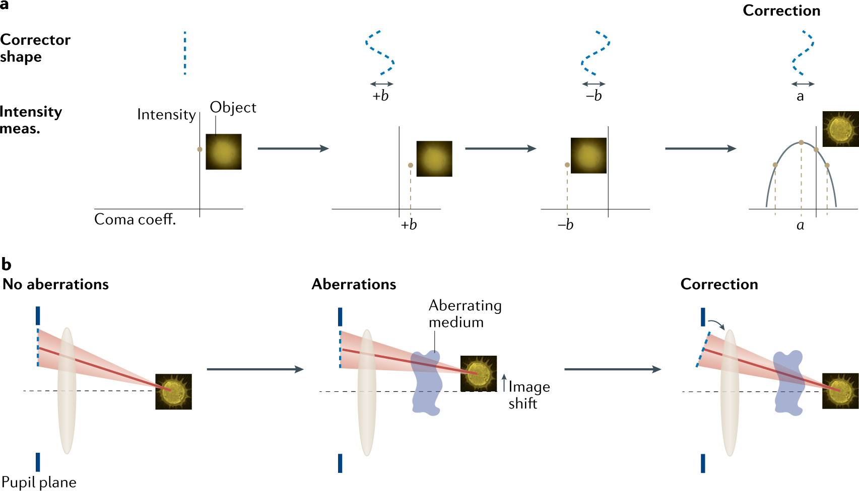
a | In modal adaptive optics (AO) schemes, different modes, which are equivalent to different shapes, are sequentially applied to the corrector. If an aberration is present such as the coma shown here, the maximum intensity will occur when the coma applied by the corrector has an equal but opposite magnitude to that introduced by the aberrating medium. Using three intensity measurements: one with the corrector introducing a plane wavefront, and one each with the corrector introducing coma with a chosen magnitude of −b or +b, the required correction can be determined using a parabolic fit to the data. b | In zonal schemes, each zone is modulated. An example of the zone-based pupil segmentation method is shown in which the required tip and tilt of each segment is determined from shifts in the image. The object is an image of a pollen grain. For simplicity only a single zone is shown but the blur in the image results from the image being shifted by different amounts by different zones owing to the aberrations. coeff., coefficient; meas., measurement.
Wavelet.
A mathematical function basis that is confined in both space and frequency.
In the zonal case, instead of considering the wavefront as consisting of aberration modes across the whole pupil, it is considered to consist of discrete non-overlapping zones. This method is often used with segmented correctors. FIGURE 4b shows an example of the pupil segmentation zonal method whereby the required tilt of each zone to correct the wavefront is determined from shifts in the image by ensuring rays meet at the focus. To ensure that the rays arriving at the focus are also in phase, the piston (equivalent to the forwards–backwards position) of each segment is determined from intensity measurements with differing amounts of piston applied70,71. Note that some wavefront correctors such as liquid crystal spatial light modulators (LCSLMs) can only perform piston modulation where the refractive index of their pixels is changed instead of mirrored segments that move back and forth. To determine the required piston introduced by each mirrored segment or pixel simultaneously, the piston for each can be modulated at a different frequency and power spectrum components can be used29. Note that indirect sensing has also been used in vision science using various different modal-based algorithms52.
Phase retrieval and phase diversity are other methods of indirect wavefront sensing72. Phase retrieval is an iterative algorithm that evaluates the local wavefront curvature from the difference in intensity between images of a point source. The simplest implementation of phase retrieval consists of acquiring two images of a fluorescent bead with different but known values of defocus and is commonly used in microscopy to correct for static aberrations introduced by the optical system30,73. Phase diversity operates on images of a spatially extended source and requires multiple phase masks at the pupil to calculate the local wavefront curvature from the difference in intensity between images. Phase diversity has been employed in astronomy to correct aberrations originating from the system, in this case the telescope itself74.
Aberration correctors
Correctors are devices that correct wavefront aberrations by changing the optical path length, which in turn modulates the wavefront. There are three main types of corrector as shown in FIG. 5. Deformable mirrors consist of a reflective surface that is either continuous (as shown in FIG. 5) or segmented. Continuous surface deformable mirrors are the most commonly employed corrector across fields. For a continuous surface mirror, when each area of its surface is pulled or pushed, a particular smooth shape known as an influence function is created. The surface shape is the sum of these influence functions. For a segmented corrector, each mirror facet can either change piston (move forwards or backwards) or change piston, tip and tilt16. Deformable mirrors flatten the wavefront using differences in physical distance travelled by the wave. LCSLMs use differences in refractive index to alter the optical path length; they can be constructed in reflective or transmissive designs75. Care must be taken when using LCSLMs as they require the use of (quasi-) monochromatic polarized light because the corrector affects wavelengths differently and is designed for use with linear polarized light. In cases where multiple wavelengths require correction, for example, in some fluorescence systems, a deformable mirror may be more appropriate as it does not suffer from chromatic effects. Deformable phase plates are fluidic devices that can change their shape based upon movement of the fluid owing to localized pressure76,77. Although current designs have far fewer actuators or pixels than deformable mirrors and LCSLMs, respectively, they are an attractive option because their size and transmissivity allow them to be easily integrated into existing imaging systems.
Fig. 5 |. Three main types of corrector.
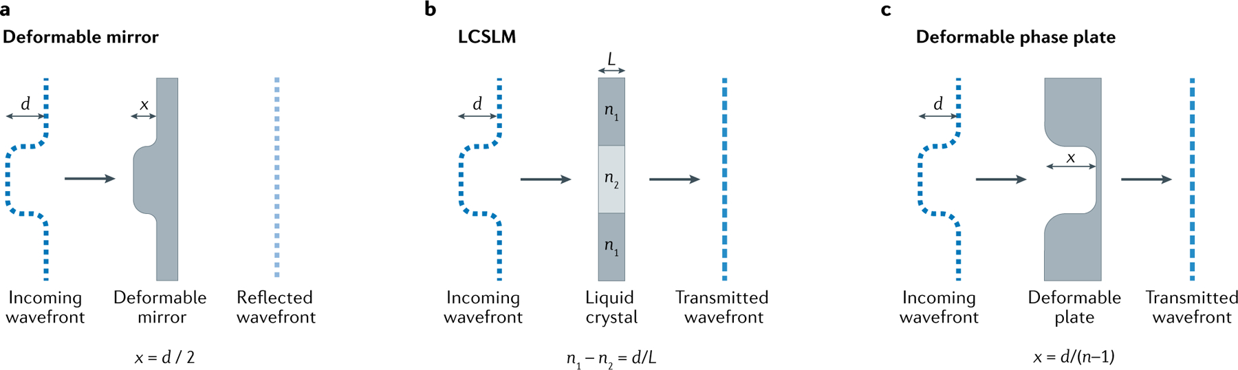
a | Deformable mirrors consist of a reflective surface that may be continuous or segmented. b | Liquid crystal spatial light modulators (LCSLMs) consist of pixels that are able to change their refractive index, n. They can be transmissive or reflective. c | Deformable phase plates are fluidic devices that are able to change their shape.
Influence function.
The shape of modulation produced by a device when a signal, such as voltage, is sent to one actuator or pixel.
Monochromatic polarized light.
Light of a single wavelength with a structured oscillation of the electric field.
TABLE 1 summarizes the typical correctors used for each field. Selecting the most suitable corrector for your application depends on the properties of the aberrations you will encounter. An important consideration is the maximum peak-to-valley of the wavefront that the device can correct. For a deformable mirror for example, this value is dictated by the stroke, which is the physical distance that an adaptive element surface can move. The maximum peak-to-valley of the wavefront that can be corrected by a deformable mirror is twice the stroke, as the additional path length is imparted to both the incident and reflected light. For example, for vision science, as discussed above, the required peak-to-valley correction is around 11 μm. Note that for segmented correctors such as LCSLMs, phase wrapping is typically used to increase the effective modulation range. Another consideration is the number of actuators (or pixels in the case of a LCSLM), which depends on the number of Zernike aberrations that will be corrected. In astronomy for example, where a significant number of Zernike aberrations are corrected, a deformable mirror with thousands of actuators may be required. Note that when considering segmented devices versus continuous surface devices, the number of required actuators can change significantly for the same aberrations78. This is related to how well a device can match the incoming wavefront. For example, for relatively smooth wavefronts, segmented devices require many more actuators. When correcting for aberrations that change rapidly with time, as is the case for ophthalmology and astronomy, the temporal response of a corrector is another factor to consider. Typically, for the aberrations of the eye, most correctors are faster than the fluctuations that need to be corrected49. By contrast, astronomical AO systems must run fast enough to keep up with the bulk flow of turbulence driven by wind above the observatory. System update rates of 1,000 Hz or faster may be required79 for best performance on bright stars, and deformable mirrors are therefore more suited as a corrector because they are generally faster than LCSLMs and deformable phase plates. There are also secondary factors that affect corrector suitability such as cost, physical size, transmissivity/reflectivity, stability and linearity. Several of the aforementioned factors relate not just to the corrector but to how the corrector interfaces with other parts of the AO system. This interfacing, termed control, is the topic of the next section.
Stroke.
Maximal physical distance that an adaptive element can move, which limits the optical path length of phase modulation that can be imparted.
Phase wrapping.
Representation of the phase information within the range [0,2π] or [−π, π] radians by adding or subtracting multiples of 2π.
Control
We discuss here some of the most important factors in calibration and control of an AO system. The main focus is on the control of continuous surface correctors using direct sensing. Note that zonal and modal wavefront control using indirect sensing is presented in FIG. 4 and so is not discussed in this section. A summary of the typical control schemes for each field can be found in TABLE 1.
Calibration.
Before operating a corrector, it is important to determine the relationship between the control signal applied to each actuator, such as the voltage, and the measured wavefront. This relationship is called the influence function. An example influence function for the central actuator of a 37-element transmissive phase plate24 is shown in FIG. 6a. The calibration procedure measures these influence functions. The corrector and sensor can be assumed to be a linear system, whereby the overall effect of the corrector on the wavefront is a linear superposition of these influence functions. It is also assumed that the sensor is linear in response.
Fig. 6 |. Influence functions and dynamic control.
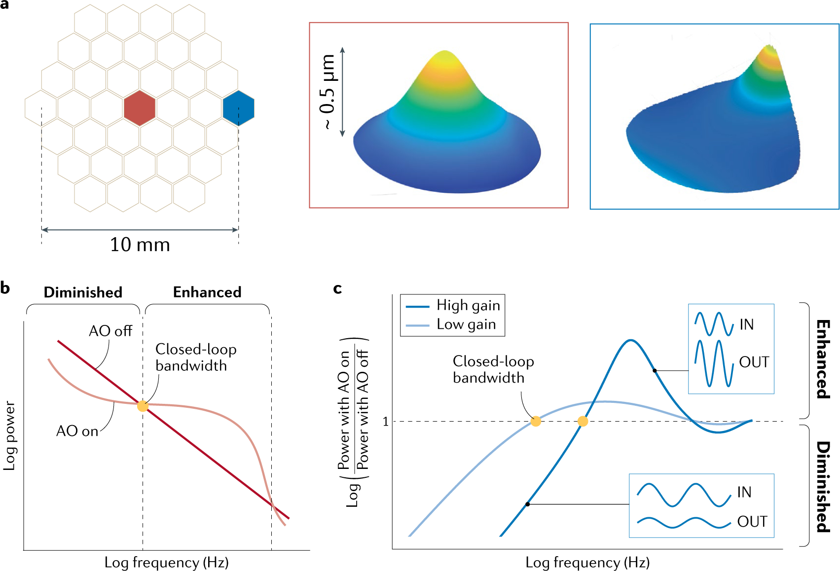
a | Actuator layout and two example influence functions for a 37-element transmissive phase plate24. b | Typical power spectrum of the fluctuations in the aberrations (root mean square (rms) wavefront error) of the eye or atmospheric turbulence with adaptive optics (AO) off, equivalent to no correction (aberrations only), and with AO on (aberrations + correction). c | The ratio of the power spectra for two gains. The closed-loop bandwidth is the maximum frequency at which the magnitude of the aberration fluctuations can be reduced (diminished). Beyond this frequency, the amplitude of the aberration fluctuations is magnified (enhanced). A higher gain results in a higher closed-loop bandwidth. Although the magnitude of a larger range of frequencies can be reduced, the higher temporal frequencies are enhanced more significantly. The curves are referred to as power rejection curves.
Implementation.
From the calibration procedure, we now have:
| (3) |
where AMeas represents a vector of aberration measurements, IF is the matrix containing the influence functions and C is a vector of control signals. AMeas can be slopes, modal coefficients, or any other measurement provided that IF is defined appropriately, that is, the influence functions are defined as slopes, modal coefficients or any other measurement. The control signals to be sent to the corrective device to generate a given wavefront can be found from:
| (4) |
where IF+ is the pseudo-inverse of the matrix containing the influence functions. IF+ is referred to as the control matrix and is often calculated using a mathematical technique for matrix inversion referred to as singular value decomposition (SVD)16. The control matrix is also referred to as the reconstructor because multiplication of this matrix by AMeas reconstructs the required control signal values. It is referred to as direct slope or modal reconstructor if the slopes or aberration coefficients are used, respectively. The advantage of SVD is that it optimizes the calculation of the inverse by removing components that can lead to instability of the system or other problems such as actuator saturation, although other methods are also available77. The required voltages to implement a given aberration mode, for an indirect sensing modal control scheme, can be calculated from Eq. 4.
Consider the general AO system shown in FIG. 1d. Before the light reaches the sensor, it first passes via the deformable mirror. Consequently, what the sensor sees is the sum of the wavefront owing to the aberrations present and the wavefront imparted by the corrector. This is referred to as a closed-loop system and is how the vast majority of AO systems are operated. If the location of the sensor is such that the light that reaches it does not pass via the corrector, it is referred to as an open-loop system. A major advantage of closed-loop systems is that the sensor checks that the wavefront imparted by the corrective device is correct. This is very important as assumptions of linearity between the signal sent to the corrector and the wavefront imparted by the corrector, as assumed during calibration, do not need to hold exactly true. Closed-loop sensor-based AO systems are typically controlled using an integral controller, although other controllers can be used16. The integral controller is implemented as:
| (5) |
where Ct are the control signals at a time t, At are the aberrations measured at a time t, and Ct0+Δt are the new control signals to be implemented. The control gain g is a value between 0 and 1 that controls the temporal response and the stability of the correction, and has an effect on which temporal frequencies can be mitigated. This is particularly important for astronomy and vision science in which the aberrations vary rapidly over short timescales, as the correction needs to keep up with the changes in the aberrations. As discussed above, the magnitude of the aberration dynamics of the eye and the atmosphere, which can be characterized by the variations in the rms wavefront error, typically follow an inverse frequency power law16,49 as shown schematically in FIG. 6b. Also shown is the residual power of the fluctuations with dynamic correction of the aberrations. The ratio of these two plots is shown in FIG. 6c and referred to as the power rejection curve.
AO systems measure and correct temporally fluctuating aberrations up to a maximum frequency, or cut-off, that defines their closed-loop bandwidth. This means that aberrations fluctuating at a frequency below the cut-off are reduced by the AO, resulting in improved image quality, while aberrations fluctuating at a frequency above the cut-off are amplified and degrade image quality. The closed-loop bandwidth is affected by many AO parameters. As an example, increasing the control gain g increases the closed-loop bandwidth but at the expense of increasingly amplifying aberration fluctuations at frequencies above this closed-loop bandwidth (FIG. 6c). Thus, an optimal trade-off is sought between the closed-loop bandwidth and gain, which is often determined using both empirical results and predictions from theory. Note that to correct for aberration fluctuations up to a given maximum defined by the closed-loop bandwidth, the aberrations must be measured and the corrector updated at significantly faster rates than the closed-loop bandwidth frequency limit. For example, to achieve good correction, astronomical AO systems require updates at around 1 kHz or more.
Closed-loop bandwidth.
The maximum frequency fluctuation that an adaptive optics system can fully or partially correct.
Results
The different applications of AO imaging have reached different levels of maturity. In astronomy, AO is routinely incorporated into new ground-based telescopes and upgrades. These are usually one-off systems that are dedicated to a particular telescope and given specific names. AO use in vision science and clinical applications continues to increase, driven by the need to elucidate structural and functional changes in the microscopic domain of the intact eye. Like astronomy applications, there is a good understanding of the nature of ophthalmic aberrations. AO in microscopy is somewhat newer and presents a different challenge with a vast range of microscope modalities and specimen types. In this section, we outline the AO optical instrumentation advances that have been made in each area. The focus of this section is on what AO can achieve in terms of image quality enhancement.
Astronomy
The original proposal for astronomical AO was made in 1953 (REF.15). After a period of development by the military, AO began to be used on astronomical telescopes and is now routinely used on large telescopes around the world. Here, we present just a few examples of such systems. For more on the history and development of AO in astronomy, see reviews by Beckers3, Davies and Kasper7, Rigaut and Neichel25, and the books by Hardy26 and Duffner80.
In astronomical AO, a star (typically called the guide star) is used as the reference for sensing the wavefront. The main source of aberrations to be corrected is atmospheric turbulence, which is blown across the telescope aperture by wind. The output of the wavefront sensor is compared with the signal expected for a flat wavefront (that is a wavefront with no turbulence) and the resultant correction is applied to a deformable mirror. The strength of the turbulence and speed of its evolution are not fixed, and AO systems are tuned to maximize correction in current conditions by adjusting the system gain (see FIG. 6c).
The Keck telescopes are among the best-known and productive general purpose astronomical AO systems, and are twin 10 m diameter segmented telescopes on the summit of Mauna Kea, Hawaii, USA. First light for AO on the Keck II telescope occurred on 4 February 1999 (REF.79) This natural guide star system was the first of a new generation of 8–10 m telescopes, delivering Strehl ratios of up to 0.37 in H band (1.6 μm) and demonstrating the dramatic improvements in image quality afforded by AO on large ground-based telescopes. The original Keck AO systems consisted of a separate tip–tilt corrector, a 349 actuator deformable mirror and a SH wavefront sensor80. The AO systems on the two telescopes were identical, and in addition to imaging and spectroscopy, AO was used to feed the Keck interferometer, which combined the light from the two telescopes. See FIG. 7a for a demonstration of Keck imaging with AO81.
Fig. 7 |. Image improvements from astronomical AO systems.
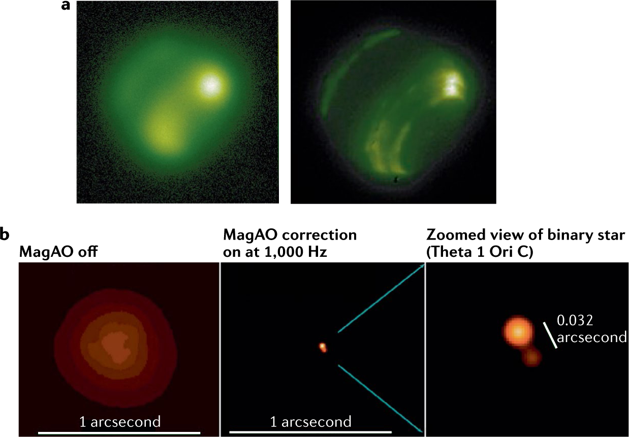
a | Early Keck adaptive optics (AO) system demonstrating the benefits of AO for astronomy. Here, Neptune is shown in a narrow filter at 1.17 μm showing methane absorption. The image on the left is uncorrected in very good 0.4 arcsec seeing. The image on the right is with AO correction81. b | Demonstration of high-resolution AO in visible light on a 6.5m telescope with Magellan AO (MagAO). The star Theta 1 Ori C is the brightest star in the Orion Trapezium cluster, a known tight binary. The left panel shows the seeing-limited image with AO off. The middle panel is the same star after closing the AO loop (AO on), with the same image field of view. Note the significant concentration of light once diffraction-limited performance is achieved. The right panel is zoomed in on the star, demonstrating the spatial resolution of AO on large telescopes92. Panel a reprinted with permission from REF.81, IOP. Panel b, image courtesy of Laird Close.
Keck AO and the Nasmyth AO System & CONICA instrument (NAOS-Conica)82,83 at the European Southern Observatory (ESO) Very Large Telescope (VLT) were instrumental in the study of the Milky Way galaxy’s supermassive black hole, which was the subject of the 2020 Nobel Prize in Physics. We further discuss the contributions of AO to this research in the Applications below.
The Keck AO systems were upgraded to use a sodium LGS, which was installed in 2001 and began science operations in 2004 on Keck II84. The LGS upgrade significantly improved sky coverage because a bright natural star was no longer required in the field. The systems received a wavefront sensor and control upgrade in 2008, which improved the sampling, frame rate and latency85. This upgrade delivered further improvements to Strehl ratio and faint star limits for natural guide star and LGS modes86.
The latest upgrades to Keck AO are currently in progress. The Keck Planet Imager and Characterizer (KPIC87) includes an IR pyramid wavefront sensor as well as a planned 1,000 actuator deformable mirror88. A key science goal for KPIC is the characterization of exoplanets orbiting late-type stars, for which the IR pyramid wavefront sensor will provide significant gains owing to the higher IR flux of such stars. As the pyramid wavefront sensor makes use of light interfered across the entire telescope pupil rather than smaller sub-apertures, it is more sensitive to low-order aberrations such as tip and tilt, focus and astigmatism than the SH sensor and takes full advantage of the diffraction limit of large telescopes89,90. Another advantage is that it provides for selectable sensitivity and dynamic range. With charge-coupled device (CCD) detectors, on-camera binning lowers the contribution of detector noise, thus allowing higher sensing speeds on fainter stars. As the dynamic range of the pyramid wavefront sensor can be adjusted by varying the modulation amplitude62, larger amplitudes provide a wider linear range while smaller amplitudes provide more sensitivity and precision. These advantages have led to the adoption of the pyramid wavefront sensor in many recent SCAO systems, including the large binocular telescope (LBT) AO systems, Subaru Coronagraphic Extreme Adaptive Optics (SCExAO), and it is under consideration for the upgrade of the Gemini Planet Imager (GPI). Furthermore, each of the coming generation of extremely large telescopes (ELTs) will be using pyramid wavefront sensors in their AO architectures.
A typical example of a more recently developed astronomical AO system is given by the Magellan AO system (MagAO). The corrector for MagAO is a 585-actuator adaptive secondary mirror (ASM), and the wavefront is sensed by a pyramid wavefront sensor (see FIG. 3d). ASMs minimize the need for compact optical relays to other deformable mirrors, thus minimizing both optical losses and the thermal background noise for IR imaging, and maximizing the field of view of the imaging system. MagAO is installed on the 6.5 m Magellan Clay telescope91 at Las Campanas Observatory in Chile. The high number of actuators in the ASM facilitates excellent correction down to visible wavelengths. As shown in FIG. 1, spatial resolution depends on wavelength, and working at visible wavelengths thus provides improved spatial resolution, which is demonstrated by MagAO in FIG. 7b (REF.92).
The above results are examples of correction derived from a single guide star in what is called SCAO. SCAO only works well for other objects near the guide star. The wavefronts from objects farther away, say 10–50 arcsec depending on wavelength, propagate through slightly different aberrations, and so will suffer from rapidly degrading correction with distance from the guide star. MCAO can significantly improve the corrected field of view. MCAO provides good correction over a wide field of view but imperfectly samples the turbulence above the telescope. Rigaut and Niechel25 provide an overview of the error sources inherent in MCAO that result in lower Strehl ratio on any single object compared with SCAO.
A wider field of view can be corrected using multiple guide stars, either natural or artificial stars created with lasers. The power of this technique is exemplified by the Multi-Conjugate Adaptive Optics Demonstrator (MAD) on the 8 m VLT in Chile. Another example of MCAO is the Gemini MCAO system (GEMS) on the Gemini South Telescope93. GEMS provides uniform sky coverage of a field as large as 85 arcsec by 85 arcsec, with sky coverage of 55%.
AO is also used for Solar astronomy94, most recently applied at the Daniel K. Inouye Solar Telescope (DKIST)95. The earliest use of AO was for observation and tracking of objects orbiting the Earth by the US military96,97.
Vision science
It has been known since at least the mid-nineteenth century that the eye contains many aberrations, but methods to effectively measure and correct them did not materialize until the end of the twentieth century. The first vision corrective methods borrowed heavily from the AO ground-based astronomical and military communities. In 1997, the first AO system was used for high-order aberration correction in the eye for both vision improvement and high-resolution retinal imaging98. Spurred by this success, AO has been integrated into various types of ophthalmoscope, principal ones being flood illumination, scanning laser ophthalmoscopy (SLO) and optical coherence tomography (OCT)10,11,99,100. Because AO is a highly scalable technology, it has been integrated into large laboratory-based ophthalmoscopes, small hand-held devices and systems designed for different species, especially human, monkey and mouse. AO is now routinely used in many scientific and clinical research laboratories around the world. For more on the history and development of AO for vision science and ophthalmology, see REFS4,101. Here, we present how AO is applied to the eye and what it can achieve.
Flood illumination.
A traditional ophthalmoscopy modality based on flash photography in which the image of the illuminated retina is captured by an area detector.
The eye’s imperfect optics and diffraction caused by the finite size of the eye’s pupil (1–8mm diameter) limit the lateral resolution at the retina to a size larger than most retinal cells and cell components and prevent their visualization. Diffraction can be minimized by dilating the pupil with mydriatic drops. However, this benefit comes at the cost of additional aberrations exposed by dilation40,46. AO increases lateral resolution by a factor of up to five over commercial ophthalmoscopes, permitting resolution of retinal details as small as 2–3 μm after pupil dilation, sufficient to resolve most major cell types in the retina including the densely packed cone photoreceptor cells in the fovea. AO also increases sensitivity as it allows a larger pupil to be used and more reflected light to be captured by the ophthalmoscope (up to a theoretical 20-fold improvement depending on pupil size and scattering properties of the retinal tissue type). This permits more-weakly reflecting retinal structures to be detected.
FIGURE 8 shows the performance of a representative AO system that was integrated into an OCT system at Indiana University21,102,103. As depicted in FIG. 8a, the AO reduces the wavefront variance of the first seven Zernike orders by two to three orders of magnitude, resulting in diffraction-limited resolution as measured by the wavefront sensor (less than λ/14 rms wavefront error). FIGURE 8b demonstrates that the AO can track and correct temporally fluctuating aberrations up to 4.5 Hz, fast enough for the vast majority of the aberrations in the eye (<2 Hz)47,48,104. Finally, FIG. 8c shows the benefit of AO for OCT retinal imaging — revealing thousands of individual cone photoreceptor cells spaced 4.5 μm apart that would otherwise not be seen. A powerful consequence of resolving cells is the ability to track them over time to observe their dynamic behaviour. It also allows images to be registered and averaged to increase signal to noise ratio over that of a single image, as illustrated in FIG. 8c and Supplementary Fig. 1.
Fig. 8 |. AO performance on a subject with high myopia.
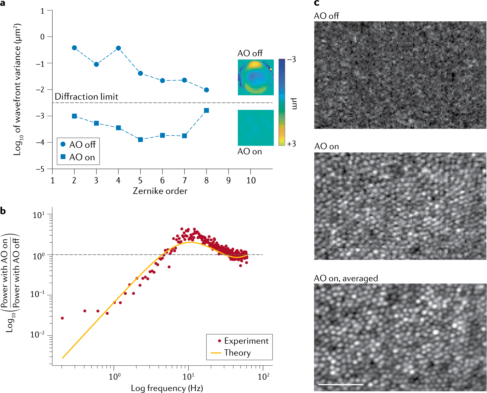
The adaptive optics (AO) system dynamically measured and corrected aberrations over a 6.7 mm pupil at the eye using a 300-lenslet Shack–Hartmann wavefront sensor, a 97-actuator deformable mirror and a direct-slope reconstructor running at a loop rate of 122 Hz REF.103. The measurement and imaging wavelength was 790 nm. The AO is part of the high-resolution AO-optical coherence tomography (OCT) imaging system developed at Indiana University21,102. A static pre-correction of −6.5 dioptres was applied to the deformable mirror to compensate for the subject’s spectacle prescription. For loop stability, control gain g was set to 0.2 and the 12 singular value decomposition (SVD) mirror modes of highest gain (most unstable) were removed from the control matrix. a | Spatial performance of the AO is quantified in terms of variance in wavefront height by Zernike order and wavefront aberration map across the eye’s pupil with AO off and on. b | Temporal performance of the AO is quantified in terms of the power rejection magnitude. Measurement and theoretical prediction are given. c | Single and averaged AO-OCT images allow visualization of cone photoreceptor cells at 1° from the fovea with AO on, but not off. By registering and averaging images acquired of the same retinal patch, the image signal to noise ratio increases and visualization of cellular structures in the image improves. Images are cropped from 1° by 1° acquired images and the scale bar is 50 μm. The associated Supplementary Video 1 shows the uncropped patch of cone photoreceptors during image acquisition with AO off and on, and Supplementary Fig. 1 shows the full extent of the registered and averaged image.
Over the past two decades, a large number of customized AO systems have been developed in the vision science community. A 2017 survey105 found that the most common AO platform in today’s ophthalmoscopes is a traditional SH wavefront sensor and a deformable mirror. This combination is used in FIG. 8. In these systems, the SH wavefront sensor typically samples a large 6.5–8 mm eye pupil with 300–600 lenslets and employs a near-IR beacon (up to a wavelength of 940 nm) to be less distracting to the individual. Although SH sensors dominate today’s ophthalmological AO systems, indirect sensing52 is garnering increased interest as it requires no hardware sensor, reducing both cost and system complexity. Numerous types of wavefront corrector (discrete-actuator deformable mirrors, LCSLMs, deformable phase plates, bimorph mirrors, magnetic membrane mirrors, microelectromechanical systems (MEMS) mirrors and combinations of these corrector types) have been tested on the eye, revealing the need for high-stroke, high-actuator-count correctors76,78. The most commonly used corrector today is a ±50 μm-stroke, 97-actuator voice-coil deformable mirror (DM97; ALPAO). The combination of a large actuator stroke and count is unique to this corrector. The ±50 μm stroke is nearly ideal, allowing correction of the refractive error in most individuals, thereby precluding the need for auxiliary lenses to correct for the individual’s spectacle prescription. The dense pattern of 97 actuators is well matched to the aberration content of the eye, delivering sharp images. However, AO does not perform well on all individuals. More challenging individuals include those with high refractive errors, unclear or highly aberrated optics owing to pathology or surgery (for example, dry eye, kerataconus, cataract, keratoplasty or refractive surgery), elevated eye motion (strabismus) and reduced fixation.
Unlike astronomical AO, the ratio of lenslets to actuators of AO systems for vision science is typically high (3:1 to 6:1). Oversampling with lenslets with a high lenslet to actuator ratio is beneficial in that it makes the measurements more robust to pupil edge effects, eye motion, system noise, drying of the tear film and other local inhomogeneities in the ocular media that can occur with ageing. Many ophthalmological AO systems use zonal control of the corrector via a direct-slope reconstructor, which has been shown to be more effective than modal control106. This is typically followed by a separate modal reconstructor for Zernike coefficients for real-time AO diagnostics during retinal image acquisition. Most laboratories develop their own AO control software or partner with laboratories that do. Open-source107 and commercial software108,109 are also available but limited.
Commercialization of AO instruments for the eye is ongoing110–112, but scientific and clinical discoveries being made with them continue to grow exponentially.
Microscopy
Adaptive optics was first extended to the field of microscopy around the year 2000. The first implementation of specimen-induced aberration compensation was in a laser scanning fluorescence confocal microscope using an indirect sensing method113. Since then, various AO schemes have been developed for a wide range of high-resolution microscopes1,2 and super-resolution fluorescence methods114 for applications ranging from neuroscience to cell biology. Although AO is becoming more widespread in the research environment, it has not yet been widely adopted in the commercial sphere.
Two types of optical field are typically involved in microscopy and can become aberrated during the imaging process — the illumination light and the emission light. Depending on the modality of the microscope, the aberrations on the wavefront of one or both optical fields need to be corrected (Supplementary Fig. 2). Most widefield microscopy, whereby emitted light propagates through the sample and forms an image on a camera (Supplementary Fig. 2a), requires aberrations to be removed from the detection path. By contrast, two-photon fluorescence microscopy, a point-scanning modality, focuses the excitation light field and collects (but does not image) emitted photons115 (Supplementary Fig. 2b). To ensure the tightest focus leading to the highest resolution, signal and contrast, aberrations of the excitation wavefront need to be removed.
The performance of some microscopy methods depends on both the excitation and emission PSFs. For example, a widefield microscopy method, lattice light sheet microscopy116, uses structured light to illuminate a single plane and image the fluorescence from this plane on a camera. Confocal microscopy scans a focused excitation laser spot across a sample and detects the emission light that passes through a pinhole, which blocks emission originating from outside the focus; its PSF is equivalent to the product of the excitation and detection PSFs. As a result, diffraction-limited focusing of both the excitation and emission light is required for optimal performance. For these methods, aberrations need to be removed from both the excitation and the emission wavefronts. In the case of lattice light sheet microscopy, because the excitation and emission wavefronts go through different objectives and experience distinct aberrations (Supplementary Fig. 2c), AO corrections have to be carried out for the two wavefronts separately.
Both the optics in the microscope itself and the samples it investigates can introduce aberrations. The optical system aberration originates from the components of the microscope and does not vary with time. Its presence can be detected from a distorted PSF, usually obtained from the image of a small fluorescent bead and derived from the PSF using phase retrieval approaches. Optical system aberration should be corrected before the imaging experiment so that only sample aberrations may degrade image quality. Sample aberrations arise from the mismatches of the sample refractive index from that of the immersion medium of the microscope objective and can severely degrade imaging performance, especially for high-resolution microscopy. Super-resolution microscopy, a collection of methods that can achieve resolution beyond the diffraction limit and reach spatial resolution of tens of nanometres, is even more sensitive to optical aberrations than the diffraction-limited methods, with biological samples a few microns thick capable of substantially reducing image quality.
Sample aberrations may vary spatially and sometimes evolve over time, for example, if imaging a developing embryo28,30,117, and must be measured and corrected in situ. AO has been extensively applied to optical microscopy to remove both system and sample aberrations. Both direct and indirect wavefront sensing methods are used for aberration measurement. For direct wavefront sensing, an SH sensor and a wavefront corrector measure and correct aberrations, respectively, and are applicable to transparent samples or to the shadow depths of opaque samples. For indirect wavefront sensing, the same corrector is typically employed for both measurement and correction of aberrations and can be applied to samples with no or substantial light scattering alike. Deformable mirrors, insensitive to polarization and having broadband high reflectivity, can efficiently remove aberrations from both illumination and emission wavefronts. For illumination that is monochromatic and polarized, LCSLMs can be applied for wavefront correction to take advantage of their large number of pixels.
By correcting both system and sample-induced aberrations, AO enables optical microscopy to achieve optimal performance in optically complex samples. Here, we list a few examples. In one example118 (FIG. 9a; Supplementary Fig. 2d), modal indirect sensing was used to measure the aberration encountered by the fluorescence emission of microtubule structures through a mammalian cell in a widefield super-resolution single-molecule localization microscope. A deformable mirror was used as the corrector to remove the cell-induced aberrations from the emitted fluorescence before image formation on a camera, which increased the number of detected fluorescent molecules and improved the measurement accuracy of their positions in 3D.
Fig. 9 |. AO in optical microscopy.
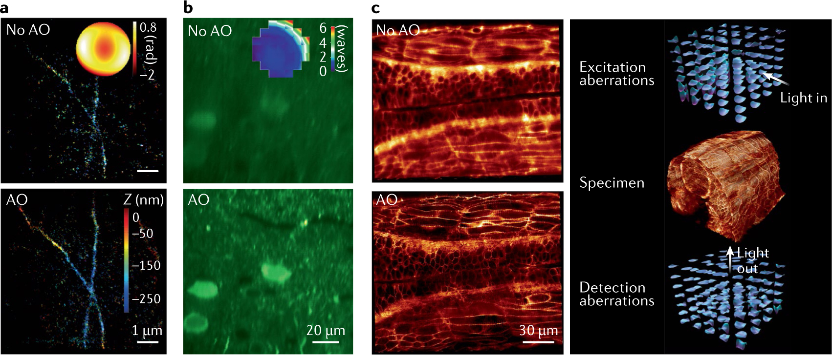
Adaptive optics (AO) correction on 3D super-resolution widefield microscopy118 (panel a), two-photon fluorescence microscopy29 (panel b) and lattice light sheet microscopy117 (panel c). Panel a reprinted with permission from REF.118 © The Optical Society. Panel b reprinted from REF.29, Springer Nature Limited. Panel c reprinted with permission from REF.117, AAAS.
In another example (FIG. 9b; Supplementary Fig. 2e), a zonal indirect sensing method was used to measure the tissue-induced aberrations when the excitation light of a two-photon fluorescence microscope travelled through a living mouse brain29. A corrective wavefront was then applied to a LCSLM to allow the formation of a diffraction-limited focus in vivo, which increased the fluorescence intensity and contrast of neurons in the brain.
Finally, AO was applied to a lattice light sheet microscope117 (FIG. 9c; Supplementary Fig. 2f) to image zebrafish embryos with a high curvature. A 1D lattice of light excited the fluorescence in a thin optical section of the sample through one objective and the emitted fluorescence was collected by another objective and imaged on a camera. Direct wavefront sensing with two SH sensors was used to measure the aberrations encountered by both the excitation and emission lights. A LCSLM was used to correct the excitation wavefront while a deformable mirror was used to correct the emission wavefront. The high speed of direct wavefront sensing measured the excitation and detection aberrations in 140 local volumes. These localized corrections were required to achieve diffraction-limited resolution throughout the image volume within the zebrafish embryo, the high curvature of which led to small isoplanatic patches.
Applications
We elaborate here on a range of applications in which the AO methods described above have been deployed to tackle imaging challenges and provide improved understanding in scientific areas ranging from the role of molecules in biological specimens to the nature of the cosmos.
Astronomy
Here, we review two of the major areas of astronomy and astrophysics affected by the use of AO, both related to night-time observations.
The Milky Way supermassive black hole.
AO has made a key contribution to the study of the supermassive black hole (SMBH) at the centre of the Milky Way galaxy. The centre of the Milky Way was long suspected to harbour a SMBH, expected to coincide with the compact radio source Sagittarius A* (see Melia and Falcke119 for a review). It was the use of AO, with the IR wavefront sensor on NACO at the VLT120 and with artificial LGSs at Keck121, that allowed the precise measurement of the mass and concentration at the centre of the Milky Way and confirmed its correspondence with Sagittarius A*. This research led to the 2020 Nobel Prize in Physics being awarded to Andrea Ghez and Reinhard Genzel for their discovery of the SMBH at the centre of our galaxy. Compared with speckle imaging techniques, AO significantly improved the image quality, dynamic range and astrometric precision of such observations122 (see FIG. 10a). Furthermore, AO has enabled spatially resolved spectroscopy123 with sufficient spectral resolution to measure the radial velocities of individual stars in the nuclear cluster of the Milky Way122,124. AO continues to make significant contributions to the study of the Milky Way SMBH — see for instance, the AO-fed GRAVITY interferometer125, which measured the gravitational redshift of a star at closest approach to the Milky Way SMBH126.
Fig. 10 |. AO in astronomy.
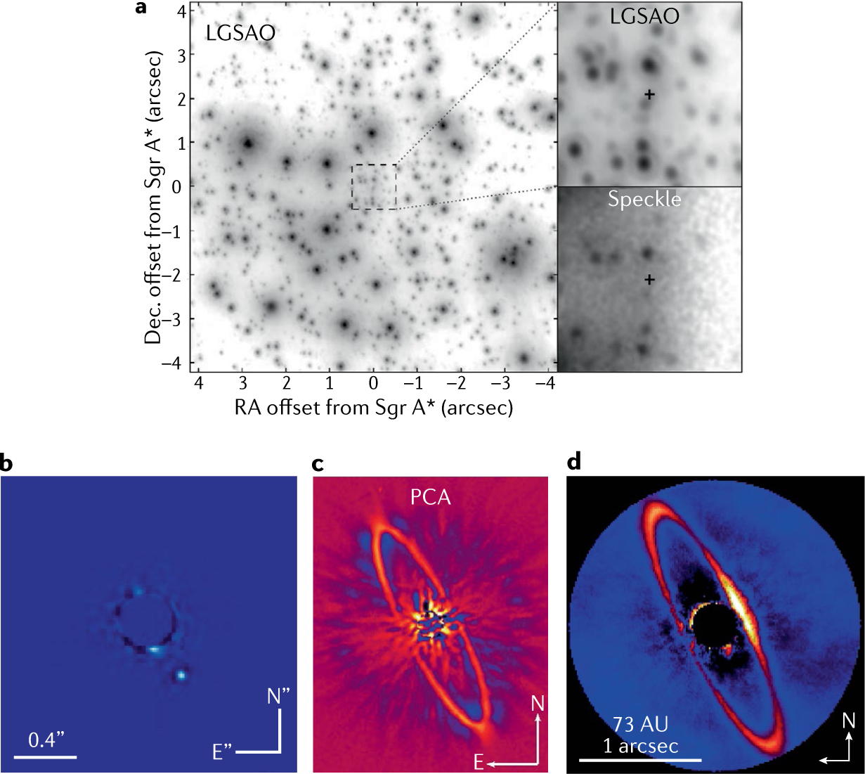
a | The centre of the Milky Way galaxy, as revealed by laser guide star adaptive optics (LGSAO) on the Keck 10 m telescopes. The right-hand panels compare speckle imaging (bottom) with the remarkable improvement in image quality and sensitivity afforded by LGSAO (top). The cross marks the location of the supermassive black hole (SMBH) at the galactic centre. AO-enabled observations such as this have been used to confirm the SMBH, measure its mass and test general relativity122. b–d | The extrasolar planet beta Pictoris b, as imaged by the Gemini Planet Imager (GPI)130. The HR 4796A debris disc as seen by the SPHERE instrument on VLT129 (panel c) and the GPI instrument on Gemini South (panel d)155. These instruments are optimized for high-contrast imaging close to bright stars to study exoplanets and circumstellar discs. The well-defined ring of the HR 4796A disc strongly suggests the presence of a planet, although none has yet been detected. Panel a reprinted with permission from REF.122, IOP. Panel b reprinted with permission from REF.130, PNAS. Panel c reprinted with permission from REF.129, EDP Science. Panel d reprinted with permission from REF.155, IOP.
Extreme AO for exoplanets and discs.
One key driver of AO performance has been the study of extrasolar planets and their environments. The first confirmed exoplanet orbiting a main sequence star, detected in the orbital reflex motion of its host star, was announced in 1995 (REF.127). This radial velocity technique and the similarly indirect transit method have accounted for most exoplanet discoveries. By their nature, the radial velocity and transit methods are biased towards close-in planets. The study of more widely separated planets can be accomplished with direct imaging, which requires AO on ground-based telescopes128.
This has led to ‘extreme’ AO (ExAO) instruments with a large number of actuators (up to 2,000 or more) and the high speed (up to 3.6 kHz) needed to image faint objects and structures next to bright stars. Two examples of such systems are the Spectro-Polarimetric High-contrast Imager for Exoplanets Research (SPHERE)129 and the GPI130.
The planetary mass object 2M1207b was imaged orbiting a brown dwarf by Chauvin et al.131. The first images of exoplanets orbiting a main sequence star were obtained by Marois et al.132 observing the star HR 8799. This star is now known to host four giant planets133, with masses of 5–7 Mjup (Mass of Jupiter). Lagrange et al.134,135 imaged a 12.7 Mjup planet orbiting beta Pictoris130 (FIG. 10b), which has been extensively studied with multiple telescopes and AO systems at wavelengths from 0.9 μm to 5 μm (REFS136–141). Likewise, the HR 8799 system has been extensively studied142–147. These many observations have allowed detailed studies of planetary atmospheres, and both the HR 8799 planets and beta Pictoris show clear orbital motion. Additional examples of well-studied directly imaged planets include HD 95086 b148, HD 106906 b149, 51 Eri b150 and PDS 70b151 and c152. For results of recent surveys, see for example REFS153,154 and Bowler128 for a broad review of the field. The study of circumstellar discs has also benefited from ExAO. Images of the HR 4796A debris disc obtained with SPHERE and GPI are shown in FIG. 10c,d129,155.
Development of ExAO systems continues. The latest generation of such high-performance exoplanet imaging AO systems include: the Subaru Coronagraphic Extreme AO system (SCExAO)156, the Magellan Extreme AO system (MagAO-X)157 and the Keck Planet Imager and Characterizer (KPIC)87. Finally, it should be noted that although ExAO seeks to deliver the highest possible Strehl ratio, it has several limitations. The highest performance is only obtainable on bright natural stars, roughly tenth magnitude and brighter. Such performance cannot be achieved with laser beacons owing to the cone effect. Very high actuator count deformable mirrors by necessity tend to be small, which limits the field of view of the imaging system. Thus, although ExAO systems are optimized for science cases such as exoplanet imaging and circumstellar disc imaging, general purpose facility AO systems do not need the same capabilities.
Vision science
The use of AO makes it possible to study thousands of cells simultaneously in the living retina and to track them longitudinally over days, months and even years. This unprecedented capability to conduct ‘living histology’ in humans is leading to new discoveries into how the retina and vision function in both healthy and diseased eyes. Furthermore, AO has an increasingly important role in how vision science is conducted and how clinicians view and interpret disease in the retina and fundus.
FIGURE 11 illustrates the breadth of AO use, showing representative images by ophthalmoscope type (AO flood illumination100,158,159, AO-scanning laser ophthalmoscopy (SLO)160–164 and AO-optical coherence tomography (OCT)10,165) and specialized sub-methods in healthy and diseased retina. How these images have been used to advance our understanding is summarized below and organized by AO ophthalmoscope type.
Fig. 11 |. Cellular-level imaging in the living human retina using different AO imaging methods.
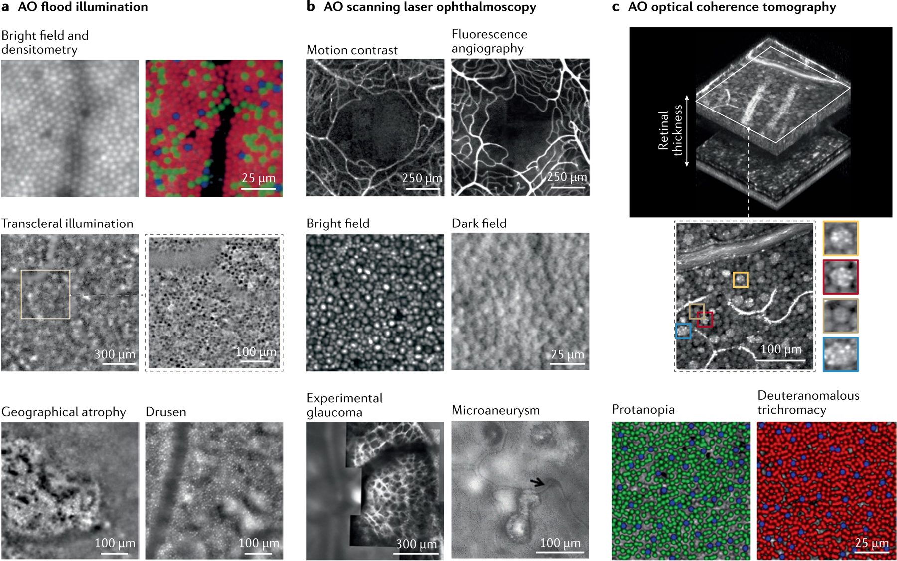
Examples shown are categorized by ophthalmoscope type: adaptive optics (AO) flood illumination100,158,159 (panel a), AO-scanning laser ophthalmoscopy (SLO)160–164 (panel b) and AO-optical coherence tomography (OCT)10,165 (panel c). Specialized methods (rows 1 and 2) and disease and colour blindness examples (row 3) are labelled under each ophthalmoscope type. Panel a (top) reprinted from REF.158, Springer Nature Limited. Panel a (middle) reprinted from REF.159, Springer Nature Limited. Panel a (bottom) reprinted with permission from REF.100, Elsevier. Panel b (top left) reprinted with permission from REF.160 © The Optical Society. Panel b (top right) reprinted with permission from REF.161, ARVO. Panel b (middle) reprinted with permission from REF.162 © The Optical Society. Panel b (bottom left) adapted from REF.163, CC BY 4.0 (https://creativecommons.org/licenses/by/4.0/). Panel b (bottom right) reprinted with permission from REF.164 © The Optical Society. Panel c (top and middle) reprinted with permission from REF.10, Annual Reviews. Panel c (bottom) reprinted with permission from REF.165, ARVO.
Flood illumination.
AO flood illumination — an extension of digital flash photography — was the first ophthalmoscope to use AO98 and the first to be commercialized with it for the clinic (rtx1; Imagine Eyes). These systems have been used extensively to image cone photoreceptors: uncovering fundamental optical properties of these cells, classifying for the first time the three cone types in human retina and revealing how disease alters the packing arrangement and other morphological properties of these cells100,158,159,166,167. The systems have also been extensively used for vascular imaging100,168,169. The recent development of trans-scleral illumination159, complementing transpupillary illumination, is expanding the use of AO flood-illumination systems to other cellular structures of the retina.
Scanning laser ophthalmoscopy.
AO-SLO — based on raster scanning a focused spot of light across the retina — has been the most extensively used ophthalmoscope for cellular-level scientific and clinical studies of the retina. Integration of multiply scattered light detection164,170–173 and single- and multiphoton fluorescence99,161,174–182 of intrinsic and extrinsic fluorophores has greatly expanded the structural and functional properties of cells that the AO-SLO can reach. AO-SLO has been used in a large number of studies99,160–164,170–185 covering fundamental cell morphology and cell populations, clinical studies of retinal disease, vision restoration, therapeutics, phototoxicity, visual function of cell types, developmental processes, and neurovascular coupling and microvascular perfusion. AO-SLO provides exceptionally detailed images of the retina in both human and animal models.
Optical coherence tomography.
Historically, AO-OCT — based on low-coherence interferometry and typically raster scanning a focused spot of light across the retina — has been a less mature technology than AO flood illumination and AO-SLO. However, it has recently undergone substantial advances, enabling it to fully use its exquisite 3D resolution and sensitivity to study the retina10,186,187. State-of-the-art AO-OCT is able to visualize label-free, highly transparent cells and cell components across the entire retinal thickness, permitting reconstruction of a 3D view of the living microscopic retina. Visualization of cells in this way is being used to track structural changes in cells on the scale of nanometres, allowing physiological processes actively occurring in the retina to be reconstructed. Numerous clinical AO-OCT studies are underway to track some of the earliest cellular changes that occur in disease, such as photoreceptors in age-related macular degeneration and retinitis pigmentosa and retinal ganglion cells in glaucoma.
Microscopy
Without the implementation of AO in microscopy, high-resolution imaging is only practically achievable in thin samples or in samples with optical properties identical to those of the immersion medium of the microscope objective such as air, water or immersion oil. This limits investigation of live biological processes to thin cultured cells or confines structural imaging of fixed samples to those with homogenized refractive index or ultrathin tissue sections. By correcting sample-induced aberrations, AO enables optical microscopy to study biological processes and structures in complex samples at high spatial resolution. Although to date the applications of AO to microscopy remain mostly proof-of-principle demonstrations, new biological discoveries have started to emerge.
When applied to cell biology, AO has made it possible to study subcellular processes in three dimensions over a broad range of length scales in live tissues. Examples include the nanoscale diffusion of clathrin-coated pits in larval zebrafish117 (FIG. 12a) as well as organelle morphology and dynamics during the development of zebrafish embryos117 (FIG. 12b). The improved spatial resolution by AO enabled the observation of growth cone dynamics in developing spinal cord, immune cell migration in a fish ear (FIG. 12c) and circulating tumour cells escaping from blood vessels in fish embryos117. For super-resolution microscopy, AO has enabled ultra-high-resolution structural imaging of subcellular structures throughout entire mammalian cells188 (FIG. 12d) and complex tissues189,190. It has also allowed dynamic super-resolution imaging of subcellular structures in live mouse and zebrafish brains73 (FIG. 12e).
Fig. 12 |. High-resolution optical microscopy with AO.
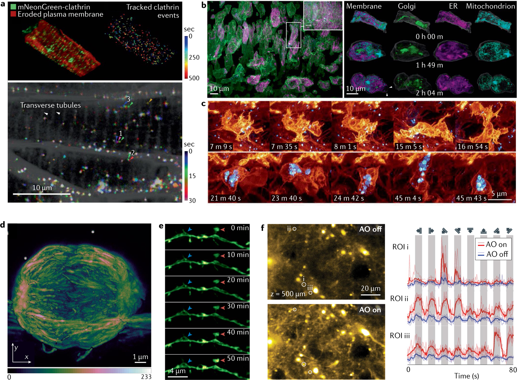
a–c | Lattice light sheet microscopy of clathrin dynamics117 (panel a), organelles morphologies and dynamics117 (panel b) and immune cell dynamics117 (panel c) in zebrafish embryos. d | 3D stimulated emission depletion microscopy of mitotic spindle (projection) in a live cell188. e | In vivo structured illumination microscopy images showing structural dynamics of a dendrite at a depth of 25 μm in the brain of a Thy1-GFP line M mouse73. f | Left: in vivo two-photon fluorescence microscopy to assess the functional calcium response of neurons to visual stimulation (500 μm inside the cortex of a living mouse). Images map the standard deviation of several hundred frames. Right: calcium transients for the regions of interest (ROIs) i–iii as a function of the direction of the grating stimuli (time)28. ER, endoplasmic reticulum. Panels a, b and c reprinted with permission from REF.117, AAAS. Panel d reprinted with permission from REF.188 © The Optical Society. Panel e reprinted from REF.73, CC BY 4.0 (https://creativecommons.org/licenses/by/4.0/). Panel f reprinted from REF.28, CC BY 4.0 (https://creativecommons.org/licenses/by/4.0/).
Clathrin.
100 nm-sized vesicles that are used to bring substances inside the cell.
Organelle.
Specialized subunit within a cell with a specific function such as the Golgi complex, the endoplasmic reticulum or the mitochondrion.
Growth cone.
Subcellular machinery used for cell migration.
The ability of AO to recover diffraction-limited PSFs in vivo is essential for the accurate characterization of functional responses of neurons in the living brain191. In these applications, microscopy is used in combination with fluorescent sensors that report neuronal activity to determine the external stimuli that neurons and their synapses selectively respond to. When imaging synapses that are hundreds of microns within the mouse brain, a dim, enlarged excitation focus caused by brain-induced aberrations leads to reduced fluorescence signal. By exciting structures outside the diffraction-limited focus, an aberrated focus also introduces contamination to the measured functional signal. By increasing the focal electric field strength, AO increases the number of detectable responsive synapses. Furthermore, it reduces the excitation focal volume and effectively removes the contamination28 (FIG. 12f). As a result, it has enabled the discovery of visual orientation-selective inputs from the thalamus to the primary visual cortex in the mouse brain192.
Synapses.
Junctions between neurons through which information flows.
Reproducibility and data deposition
To reproduce AO systems and their data, it is vital that information is shared. This section discusses the sharing of information in each field.
Astronomy
Most large observatories maintain publicly accessible data archives. The astronomers who proposed and were awarded telescope time are typically granted a proprietary period after observations, for example, 18 months, during which they have exclusive access for analysis and publication. After this period, the data become public and anyone in the world may download them. Such archives include the Gemini Science Archive, the Keck Observatory Archive, the Subaru Telescope Archive System and the ESO Science Archive Facility.
AO instruments often provide data reduction tutorials, guides and software to facilitate user processing of data. Examples include the Keck NIRC2 imager, SPHERE and GPI.
Vision science
Early in the development of AO systems for the eye, it was recognized that a common language was needed to report system performance to facilitate reproducibility. In 2002, the vision science community established a universally accepted naming convention for reporting Zernike coefficients as defined by the OSA ANSI standard37. More recently, many laboratories have converged on a common AO design and integration into the ophthalmoscope. Much of the information about these designs is shared: specific hardware, flowcharts and performance specifications of the control software, and schematics of the system optical layout. To reproduce a system requires additional information, namely the actual control software developed and the commercial optical ray tracing design.
The use of a common language and standardized designs has greatly improved the reporting and comparing of performance results. There has been extensive reproducibility of ocular aberration measurements and retinal imaging results across different AO ophthalmoscopes and laboratories. Population studies involving thousands of individuals using SH aberrometry have been compared and have demonstrated good agreement46. Practically every AO ophthalmoscope built has been used to image cone photoreceptors at different locations in the retina, the density and spacing of which are routinely compared with widely accepted measurements obtained in in vivo imaging193–195 and histological196 studies.
Data deposition of AO technology for vision science continues to be in the peer-reviewed literature. This includes an entire textbook devoted to the topic4 and a recent survey of experts on the state of the field, covering system design, use and future directions105. Data deposition of results with AO instruments is increasing, driven in part by US federal agency data management and sharing policies. These depositions are more challenging than in astronomy and microscopy as they must follow strict institutional review board rules to protect individual confidentiality.
Microscopy
The diverse and often live samples investigated by in-house microscopy systems make it difficult to have quantitative comparisons of different AO and microscope modalities. However, the underlying biological principles remain the same. With the increasing application of AO to microscopy, the new biological insights that AO enables will be tested and validated by multiple laboratories. The increasingly widespread requirement of making raw data and custom codes available at online repositories also provides public access to materials beyond those discussed in research papers, which would enable more in-depth analysis and understanding of the published results by general practitioners of optical microscopy. Although raw data are often made publicly available through university-specific platforms and custom codes through GitHub, reproducibility in AO microscopy would be improved by a more systematic sharing of control and analysis software. Effective dissemination of know-how is also essential to help make AO more accessible to non-experts who wish to use it in their microscopy applications. Websites collating tutorials and experimental protocols, such as AOmicroscopy, help by making available a broad range of information at different levels of complexity and detail, again not customarily provided by research papers.
Limitations and optimizations
Current AO systems share common limitations, in particular anisoplanatism. In this section, we present how these limitations vary and are optimized across fields.
Astronomy
There are three main limitations for astronomical AO. The first limitation is the number of controlled degrees of freedom, nominally set by the number of actuators on the corrector, but also the architecture of the wavefront sensor and control system. This ‘fitting error’ describes how much turbulence is not corrected.
The second limitation is set by the balance of noise and time lag. The AO system must run at finite speed owing to photon and detector noise. Different wavefront sensor architectures have different spatial frequency-dependent responses to noise, and wavefront sensor detector choice is important to balance speed versus readout noise. Additionally, readout, computation and application of correction require finite times. Since turbulence is constantly evolving, the delay between measurement and application causes a correction error. Speed and gain optimization balance the contributions of noise and lag. Further trade-offs can be made with fitting error, both in design and during operation.
The third limitation is the volume of the atmosphere sampled by a given reference. The wavefront from a nearby object propagates through slightly different turbulence, causing a relative error in correction. This angular anisoplanatism error limits the well-corrected field of view to, depending on wavelength and conditions, on the order of 1–30 arcsec. This limits the sky coverage of AO systems owing to the relative rarity of stars bright enough for good correction and limits the number of targets and science cases for which AO can be used. Anisoplanatism can be mitigated through the use of artificial LGSs84 and using MCAO techniques25. Other forms of anisoplanatism include focal anisoplanatism or ‘the cone effect’, from the finite height of a LGS beacon causing only a cone-shaped region of the atmosphere to be sampled; and tilt anisoplanatism, due to an offset tip–tilt reference being used during LGS operations, which suffers a different tip and tilt from the target object.
Detailed discussions of these limits can be found in REFS3,26.
Vision science
The ability of AO to work in a clinical setting remains the most pressing need. Alignment of the eye and AO operation must occur within seconds of the individual being placed in front of the instrument, and AO must work effectively and robustly regardless of individual. Unfortunately, the large variation in eyes and visual performance between individuals makes good AO performance challenging. In particular, older eyes and diseased eyes are generally more difficult to image — they have smaller pupils, more frequent drying of the tear film, increased aberrations, eye motion and ocular obstructions (for example, cataracts), and often have intraocular lenses. The optical properties of the retina also vary, even in healthy individuals, complicating the beacon that scatters back from the retina and is sensed by AO. Addressing these variations with smarter AO control algorithms that operate more efficiently and reliably will go a long way towards improving clinical use, but these remain a work in progress. Furthermore, best practices of AO control have yet to be established, even at the level of optimal centroiding and handling of SH wavefront sensor spots.
AO is also limited to the eye’s isoplanatic patch size (~1°), which is much smaller than images acquired with clinical ophthalmoscopes (>20°)27. MCAO can increase this size197,198 but adds significant complexity. AO also produces a narrow depth of focus, which extends over a relatively small fraction of the total retinal thickness. This requires the same retinal patch to be reimaged multiple times with different focus, thus imposing serious restrictions on imaging studies; no effective solution has been found. Ocular chromatic aberrations199, light safety200 and the high cost and complexity of AO technology pose additional challenges to AO ophthalmoscopes. Finally, the benefit of AO is ultimately limited by the diffraction caused by the finite size of the eye pupil. Incremental improvements in resolution have been shown using, for example, sub-Airy disc confocal pinhole detection201, but substantive improvements will require super-resolution methods202,203.
Microscopy
The heterogeneity in refractive index as well as the sometimes high surface curvature of biological samples can lead to small isoplanatic patch size. Direct wavefront sensing can be achieved at high speed and thus allows region-specific AO corrections to be applied throughout 3D volumes for maximal resolution recovery30,117. An alternative approach is MCAO, whereby correctors conjugate to different aberrating layers are used to increase the size of the isoplanatic patch in a similar way to astronomy. Methods based on comparable principles have been applied to microscopy, where enlargement of the isoplanatic patch has been demonstrated in samples with a well-defined, dominant aberrating layer32,204. However, because most biological samples introduce aberrations continuously throughout the specimen volume, it remains to be seen whether MCAO leads to much reduced anisoplanatism. For these samples, continued developments in both methodology and wavefront corrector technology are needed, with the ideal correctors having pixels distributed in 3D to match the aberration profile of the sample. Finally, AO methods discussed in this Primer aim to correct aberrations but not scattering. Wavefront shaping has been applied to scattering control in opaque samples — an active research area that has been reviewed recently205–207.
Outlook
The future of astronomical AO is apparent in plans for the coming generation of the 25–39 m extremely large telescopes (ELTs). These are the 25 m Giant Magellan Telescope (GMT)208, the Thirty Meter Telescope (TMT)209 and the European Extremely Large Telescope (E-ELT)210. Compared with existing 5–10 m AO equipped observatories, these telescopes will offer ground-breaking improvements in diffraction-limited resolution and sensitivity. The ELTs are each planned to have integrated AO systems, both for high Strehl ratio natural guide star operations and with multiple lasers for wider field corrections and higher sky coverage211–213.
The widespread adoption of AO for biological imaging (in terms of both microscopy and vision science) relies on making systems more compact, less expensive and easier to use. For aberration sensing, compactness is achieved with indirect sensing approaches as they circumvent the need for additional hardware but at the cost of increased interfacing with the image acquisition system. With respect to aberration correction, the most widely used correctors are reflective. Integrating these reflective devices into an existing system, bespoke or commercial, is not trivial and cannot necessarily be achieved compactly if an additional conjugated plane has to be appended to the original system and if the optical incidence angle on the device has to be optimized to achieve maximal performance. The development of transmissive wavefront shaping devices should enable AO systems to be fully integrated as they can be more simply slotted into imaging systems without any increase in footprint77. Transmissive wavefront shaping devices would make a significant difference in MCAO because such devices could potentially be stacked up and substantially simplify experimental systems. For now, reflective devices are still preferred because they are better able to shape light for optimal aberration corrections with a higher number of controllable elements and a larger phase-shift compared with transmissive devices.
In addition to developments in hardware, numerical methods will also have an important role in the future of AO technology. The rapidly growing field of artificial intelligence is of particular interest to AO. Substantial effort has recently been dedicated to devising machine learning algorithms capable of evaluating wavefront aberrations. It is anticipated that machine learning will help to minimize the number of measurements required for indirect sensing methods without additional instrumentation, thus allowing simplification of the overall system while simultaneously widening its scope of applications. Machine learning for wavefront sensing has been successfully demonstrated in several AO fields using point objects and for retinal imaging214–217 or for aberration prediction in astronomy218. However, significant work remains to be done before machine learning can be applied to more complex specimens and implemented in distributable packages for universal usage. One of the main challenges to overcome is the need for large data in the learning step combined with the sensitivity of the outcome depending on system-specific experimental conditions. Although these recent advances are exciting, numerical AO methods are not novel. Indeed, computational AO was proposed more than 20 years ago for correcting aberrations by mapping the refractive index distribution, modelling the aberrations through ray tracing and then correcting the effects of the aberrations using deconvolution219. Although determining the refractive index distribution is not practically possible for most systems, it has been demonstrated for OCT and the results used to tomographically reconstruct the aberrated wavefront and apply correction using a standard wavefront shaping device or through image post-processing220. Phase diversity approaches can also be used computationally to remove aberrations in fluorescence images221. Physical correction is preferred over deconvolution because the additional measurement of the corrected image yields additional photons, substantially increasing the signal to noise ratio and also validating the quality of the corrective process; this fact applies to AO in general and should not be understated.
In this Primer, we primarily discussed AO in the context of high-resolution imaging but there are numerous non-imaging applications in which implementing AO has or will yield substantial benefits. Free-space communications is one of them222. Similar challenges to astronomical imaging are encountered in satellite–Earth communications because the signal has to traverse the atmosphere to reach the Earth’s surface. However, the two areas differ in that the source signal can be controlled in space communications and a beacon embedded to facilitate sensing. Beyond the atmosphere, other turbulent gas and liquid mixtures will have dynamic variations in pressure similar to those in the atmosphere, and that includes oceans. AO can therefore be deployed for exploration and communications through oceanic turbulence in a manner analogous to astronomy and space communications223. Another non-imaging area of application for AO is laser processing of materials224. Laser processing by focusing ultrafast pulses using a high numerical aperture lens is highly susceptible to optical aberrations owing to the nonlinearity of the mechanisms at play, for example, in ablation/writing and multiphoton polymerization. AO is thus key to large-scale industrial deployment of the technology. Although the implementation of AO for processing has similarities to that in microscopy, the relatively better-known geometry and optical properties of samples in laser processing simplify the sensing step and allow wavefront control technology for more advanced applications such as parallel and extend-depth-of-field writing224. Another non-imaging field in which AO has been employed is for the optimization of high-power laser beam control225. Finally, a link must be drawn between AO and wavefront control in complex media. The latter aims at compensating the effect of multiple scattering events and therefore will involve the correction of aberrations containing high spatial frequency207. By contrast, AO has primarily been concerned with low spatial frequency aberrations. It will be important for future AO and scattering correction technology to bridge this gap and operate across spatial frequency length scales.
Supplementary Material
Acknowledgements
D.T.M. and K.K. acknowledge support from the NIH grants R01 EY018339 and R01 EY029808. N.J. acknowledges support from the NIH grant U01NS103489. M.J.B., K.M.H. and R.T. acknowledge support from the European Research Council 695140.
Footnotes
Competing interests
D.T.M. and K.K. have a patent on AO-OCT technology. Both authors stand to benefit financially from any commercialization of the technology. N.J. has two patents on AO microscopy technology. M.J.B. holds patents on adaptive optics technology and has significant interests in the companies Opsydia Ltd and Aurox Ltd. Otherwise, the authors are not aware of any affiliations, memberships, funding or financial holdings that might be perceived as affecting the objectivity of this publication. K.M.H., R.T. and J.R.M. declare no competing interests.
Peer review information
Nature Reviews Methods Primers thanks V. Chambouleyron, B. Neichel and the other, anonymous, reviewer(s) for their contribution to the peer review of this work.
Supplementary information
The online version contains supplementary material available at https://doi.org/10.1038/s43586-021-00066-7.
Related links
AOmicroscopy: https://aomicroscopy.org/
GPI: http://docs.planetimager.org/pipeline/
Keck NIRC2 imager: https://www2.keck.hawaii.edu/inst/nirc2/post_observing.html
SPHERE: http://www.eso.org/sci/software/pipelines/
The Gemini Science Archive: https://archive.gemini.edu/searchform
The Keck Observatory Archive: https://www2.keck.hawaii.edu/koa/public/koa.php
The Subaru Telescope Archive System: https://stars2.naoj.hawaii.edu/stars1min.html
The ESO Science Archive Facility: http://archive.eso.org/cms.html
References
- 1.Booth MJ Adaptive optical microscopy: the ongoing quest for a perfect image. Light. Sci. Appl. 3, e165 (2014). [Google Scholar]
- 2.Ji N Adaptive optical fluorescence microscopy. Nat. Methods 14, 374–380 (2017). [DOI] [PubMed] [Google Scholar]
- 3.Beckers JM Adaptive optics for astronomy: principles, performance, and applications. Annu. Rev. Astron. Astr. 31, 13–62 (1993). [Google Scholar]
- 4.Porter J, Queener HM, Lin JE, Thorn K & Awwal A Adaptive Optics for Vision Science: Principles, Practices, Design and Applications (Wiley, 2006). [Google Scholar]
- 5.Kubby J, Gigan S & Cui M Adaptive Optical Microscopy for Biological Imaging (Cambridge Univ. Press, 2019). [Google Scholar]
- 6.Roddier F Adaptive Optics in Astronomy (Cambridge Univ. Press, 1999). [Google Scholar]
- 7.Davies R & Kasper M Adaptive optics for astronomy. Annu. Rev. Astron. Astr. 50, 305–351 (2012). [Google Scholar]
- 8.Ji N, Sato TR & Betzig E Characterization and adaptive optical correction of aberrations during in vivo imaging in the mouse cortex. Proc. Natl Acad. Sci. USA 109, 22–27 (2012). [DOI] [PMC free article] [PubMed] [Google Scholar]
- 9.Liu R, Li Z, Marvin JS & Kleinfeld D Direct wavefront sensing enables functional imaging of infragranular axons and spines. Nat. Methods 16, 615–618 (2019). [DOI] [PMC free article] [PubMed] [Google Scholar]
- 10.Miller DT & Kurokawa K Cellular scale imaging of transparent retinal structures and processes using adaptive optics optical coherence tomography. Annu. Rev. Vis. Sci. 6, 115–148 (2020). [DOI] [PMC free article] [PubMed] [Google Scholar]
- 11.Burns SA, Elsner AE, Sapoznik KA, Warner RL & Gast TJ Adaptive optics imaging of the human retina. Prog. Retin. Eye Res. 68, 1–30 (2019). [DOI] [PMC free article] [PubMed] [Google Scholar]
- 12.Georgiou M et al. Adaptive optics imaging of inherited retinal diseases. Brit. J. Ophthalmol. 102, 1028 (2018). [DOI] [PMC free article] [PubMed] [Google Scholar]
- 13.Roorda A & Duncan JL Adaptive optics ophthalmoscopy. Annu. Rev. Vis. Sci. 1, 1–32 (2014). [DOI] [PMC free article] [PubMed] [Google Scholar]
- 14.Gill JS, Moosajee M & Dubis AM Cellular imaging of inherited retinal diseases using adaptive optics. Eye 33, 1683–1698 (2019). [DOI] [PMC free article] [PubMed] [Google Scholar]
- 15.Babcock HW The possibility of compensating astronomical seeing. Publ. Astron. Soc. Pac. 65, 229 (1953). [Google Scholar]
- 16.Tyson RK Principles of Adaptive Optics (CRC Press, 2015). [Google Scholar]
- 17.Vangindertael J et al. An introduction to optical super-resolution microscopy for the adventurous biologist. Methods Appl. Fluores. 6, 022003 (2018). [DOI] [PubMed] [Google Scholar]
- 18.Dai Y et al. Active compensation of extrinsic polarization errors using adaptive optics. Opt. Express 27, 35797–35810 (2019). [DOI] [PubMed] [Google Scholar]
- 19.He C, Hu Q, Dai Y & Booth MJ Vectorial adaptive optics - correction of polarization and phase. in Adaptive Optics and Wavefront Control for Biological Systems VI Vol. 11248 1124808 (OSA Publishing, 2020). [Google Scholar]
- 20.Felberer F, Kroisamer J-S, Hitzenberger CK & Pircher M Lens based adaptive optics scanning laser ophthalmoscope. Opt. Express 20, 17297–17310 (2012). [DOI] [PubMed] [Google Scholar]
- 21.Liu Z, Kocaoglu OP & Miller DT In-the-plane design of an off-axis ophthalmic adaptive optics system using toroidal mirrors. Biomed. Opt. Express 4, 3007–3029 (2013). [DOI] [PMC free article] [PubMed] [Google Scholar]
- 22.Young LK, Morris TJ, Saunter CD & Smithson HE Compact, modular and in-plane AOSLO for high-resolution retinal imaging. Biomed. Opt. Express 9, 4275–4293 (2018). [DOI] [PMC free article] [PubMed] [Google Scholar]
- 23.Thaung J, Knutsson P, Popovic Z & Owner-Petersen M Dual-conjugate adaptive optics for wide-field high-resolution retinal imaging. Opt. Express 17, 4454–4467 (2009). [DOI] [PubMed] [Google Scholar]
- 24.Hampson KM et al. Closed-loop multiconjugate adaptive optics for microscopy. in Adaptive Optics and Wavefront Control for Biological Systems VI Vol. 11248 1124809 (OSA Publishing, 2020). [Google Scholar]
- 25.Rigaut F & Neichel B Multiconjugate adaptive optics for astronomy. Annu. Rev. Astron. Astr. 56, 277–314 (2018). [Google Scholar]
- 26.Hardy JW Adaptive Optics for Astronomical Telescopes (Oxford Univ. Press, 1998). [Google Scholar]
- 27.Bedggood P, Daaboul M, Ashman R, Smith G & Metha A Characteristics of the human isoplanatic patch and implications for adaptive optics retinal imaging. J. Biomed. Opt. 13, 024008 (2008). [DOI] [PubMed] [Google Scholar]
- 28.Wang K et al. Direct wavefront sensing for high-resolution in vivo imaging in scattering tissue. Nat. Commun. 6, 7276 (2015). [DOI] [PMC free article] [PubMed] [Google Scholar]
- 29.Wang C et al. Multiplexed aberration measurement for deep tissue imaging in vivo. Nat. Methods 11, 1037–1040 (2014). [DOI] [PMC free article] [PubMed] [Google Scholar]
- 30.Wang K et al. Rapid adaptive optical recovery of optimal resolution over large volumes. Nat. Methods 11, 625–628 (2014). [DOI] [PMC free article] [PubMed] [Google Scholar]
- 31.Lin R, Kipreos ET, Zhu J, Khang CH & Kner P Subcellular three-dimensional imaging deep through multicellular thick samples by structured illumination microscopy and adaptive optics. Nat. Comm. 12, 3148 (2021). [DOI] [PMC free article] [PubMed] [Google Scholar]
- 32.Mertz J, Paudel H & Bifano TG Field of view advantage of conjugate adaptive optics in microscopy applications. Appl. Opt. 54, 3498–3506 (2015). [DOI] [PMC free article] [PubMed] [Google Scholar]
- 33.Wilson RN, Franza F & Noethe L Adaptive optics: I. A system for optimizing the optical quality and reducing the costs of large telescopes. J. Mod. Opt. 34, 485–509 (1987). [Google Scholar]
- 34.Lakshminarayanan V & Fleck A Zernike polynomials: a guide. J. Mod. Optic. 58, 1678–1678 (2011). [Google Scholar]
- 35.Noll RJ Zernike polynomials and atmospheric turbulence. J. Opt. Soc. Am. 66, 207–210 (1976). [Google Scholar]
- 36.Hampson K, Antonello J, Lane R & Booth M Sensorless adaptive optics. Zenodo; 10.5281/zenodo.4066425 (2020). [DOI] [Google Scholar]
- 37.Thibos LN et al. Standards for reporting the optical aberrations of eyes. J. Refract. Surg. 18, S652–S660 (2002). [DOI] [PubMed] [Google Scholar]
- 38.Kolmogorov AN Dissipation of energy in the locally isotropic turbulence. Proc. R. Soc. Lond. Math. Phys. Sci 434, 15–17 (1991). [Google Scholar]
- 39.Kolmogorov AN The local structure of turbulence in incompressible viscous fluid for very large Reynolds numbers. Proc. R. Soc. Lond. Math. Phys. Sci 434, 9–13 (1991). [Google Scholar]
- 40.Thibos LN, Hong X, Bradley A & Cheng X Statistical variation of aberration structure and image quality in a normal population of healthy eyes. J. Opt. Soc. Am. A 19, 2329 (2002). [DOI] [PubMed] [Google Scholar]
- 41.Devaney N et al. Correction of ocular and atmospheric wavefronts: a comparison of the performance of various deformable mirrors. Appl. Opt. 47, 6550 (2008). [DOI] [PubMed] [Google Scholar]
- 42.Cantalloube F et al. Wind-driven halo in high-contrast images. Astron. Astrophys. 638, A98 (2020). [Google Scholar]
- 43.Males JR & Guyon O Ground-based adaptive optics coronagraphic performance under closed-loop predictive control. J. Astron. Telesc. Instrum. Syst. 4, 019001 (2018). [Google Scholar]
- 44.Conan J-M, Rousset G & Madec P-Y Wave-front temporal spectra in high-resolution imaging through turbulence. J. Opt. Soc. Am. A 12, 1559–1570 (1995). [Google Scholar]
- 45.Roddier F, Roddier D, Northcott MJ, Graves JE & McKenna DL One-dimensional spectra of turbulence-induced Zernike aberrations: time-delay and isoplanicity error in partial adaptive compensation. J. Opt. Soc. Am. A 10, 957–965 (1993). [Google Scholar]
- 46.Salmon TO & van de Pol C Normal-eye Zernike coefficients and root-mean-square wavefront errors. J. Cataract. Refract. Surg. 32, 2064–2074 (2006). [DOI] [PubMed] [Google Scholar]
- 47.Hofer H, Artal P, Singer B, Aragón JL & Williams DR Dynamics of the eye’s wave aberration. J. Opt. Soc. Am. A 18, 497 (2001). [DOI] [PubMed] [Google Scholar]
- 48.Diaz-Santana L, Torti C, Munro I, Gasson P & Dainty C Benefit of higher closed-loop bandwidths in ocular adaptive optics. Opt. Express 11, 2597–2605 (2003). [DOI] [PubMed] [Google Scholar]
- 49.Jarosz J et al. High temporal resolution aberrometry in a 50-eye population and implications for adaptive optics error budget. Biomed. Opt. Express 8, 2088–2105 (2017). [DOI] [PMC free article] [PubMed] [Google Scholar]
- 50.Schmitt JM & Kumar G Turbulent nature of refractive-index variations in biological tissue. Opt. Lett. 21, 1310–1312 (1996). [DOI] [PubMed] [Google Scholar]
- 51.Porter J, Guirao A, Cox IG & Williams DR Monochromatic aberrations of the human eye in a large population. J. Opt. Soc. Am. A 18, 1793–1803 (2001). [DOI] [PubMed] [Google Scholar]
- 52.Verstraete HRGW et al. Wavefront sensorless adaptive optics OCT with the DONE algorithm for in vivo human retinal imaging [Invited]. Biomed. Opt. Express 8, 2261–2275 (2017). [DOI] [PMC free article] [PubMed] [Google Scholar]
- 53.Shack RV & Platt BC Production and use of a lenticular Hartmann screen. J. Opt. Soc. Am. 61, 656–660 (1971). [Google Scholar]
- 54.Thomas S et al. Comparison of centroid computation algorithms in a Shack–Hartmann sensor. Mon. Not. R. Astron. Soc. 371, 323–336 (2006). [Google Scholar]
- 55.Geng Y et al. Optical properties of the mouse eye. Biomed. Opt. Express 2, 717–738 (2011). [DOI] [PMC free article] [PubMed] [Google Scholar]
- 56.Akondi V & Dubra A Multi-layer Shack-Hartmann wavefront sensing in the point source regime. Biomed. Opt. Express 12, 409–432 (2021). [DOI] [PMC free article] [PubMed] [Google Scholar]
- 57.Rahman SA & Booth MJ Direct wavefront sensing in adaptive optical microscopy using backscattered light. Appl. Opt. 52, 5523–5532 (2013). [DOI] [PubMed] [Google Scholar]
- 58.Poyneer LA Scene-based Shack-Hartmann wavefront sensing: analysis and simulation. Appl. Opt. 42, 5807–5815 (2003). [DOI] [PubMed] [Google Scholar]
- 59.Ashida Y et al. Imaging performance of microscopy adaptive-optics system using scene-based wavefront sensing. J. Biomed. Opt. 25, 123707 (2020). [DOI] [PMC free article] [PubMed] [Google Scholar]
- 60.Tatulli E & Ramaprakash AN Laser tomography adaptive optics: a performance study. J. Opt. Soc. Am. A 30, 2482 (2013). [DOI] [PubMed] [Google Scholar]
- 61.Laslandes M, Salas M, Hitzenberger CK & Pircher M Influence of wave-front sampling in adaptive optics retinal imaging. Biomed. Opt. Express 8, 1183–1200 (2017). [DOI] [PMC free article] [PubMed] [Google Scholar]
- 62.Ragazzoni R Pupil plane wavefront sensing with an oscillating prism. J. Mod. Opt. 43, 289–293 (1996). [Google Scholar]
- 63.Engler B, Weddell S & Clare R Wavefront sensing with prisms for astronomical imaging with adaptive optics. in 2017 International Conference on Image and Vision Computing New Zealand 1–7 (IEEE, 2017). [Google Scholar]
- 64.Chamot SR, Dainty C & Esposito S Adaptive optics for ophthalmic applications using a pyramid wavefront sensor. Opt. Express 14, 518–526 (2006). [DOI] [PubMed] [Google Scholar]
- 65.Iglesias I Pyramid phase microscopy. Opt. Lett. 36, 3636–3638 (2011). [DOI] [PubMed] [Google Scholar]
- 66.Berto P, Rigneault H & Guillon M Wavefront sensing with a thin diffuser. Opt. Lett. 42, 5117–5120 (2017). [DOI] [PubMed] [Google Scholar]
- 67.Nishizaki Y et al. Deep learning wavefront sensing. Opt. Express 27, 240–251 (2019). [DOI] [PubMed] [Google Scholar]
- 68.Antonello J, Barbotin A, Chong EZ, Rittscher J & Booth MJ Multi-scale sensorless adaptive optics: application to stimulated emission depletion microscopy. Opt. Express 28, 16749–16763 (2020). [DOI] [PMC free article] [PubMed] [Google Scholar]
- 69.Facomprez A, Beaurepaire E & Débarre D Accuracy of correction in modal sensorless adaptive optics. Opt. Express 20, 2598–2612 (2012). [DOI] [PubMed] [Google Scholar]
- 70.Ji N, Milkie DE & Betzig E Adaptive optics via pupil segmentation for high-resolution imaging in biological tissues. Nat. Methods 7, 141–147 (2009). [DOI] [PubMed] [Google Scholar]
- 71.Milkie DE, Betzig E & Ji N Pupil-segmentation-based adaptive optical microscopy with full-pupil illumination. Opt. Lett. 36, 4206–4208 (2011). [DOI] [PubMed] [Google Scholar]
- 72.Gonsalves RA Phase retrieval and diversity in adaptive optics. Opt. Eng. 21, 215829 (1982). [Google Scholar]
- 73.Turcotte R et al. Dynamic super-resolution structured illumination imaging in the living brain. Proc. Natl Acad. Sci. USA 116, 9586–9591 (2019). [DOI] [PMC free article] [PubMed] [Google Scholar]
- 74.Sauvage J-F, Fusco T, Rousset G & Petit C Calibration and precompensation of noncommon path aberrations for extreme adaptive optics. J. Opt. Soc. Am. A 24, 2334–2346 (2007). [DOI] [PubMed] [Google Scholar]
- 75.Maurer C, Jesacher A, Bernet S & Ritsch-Marte M What spatial light modulators can do for optical microscopy. Laser Photonics Rev. 5, 81–101 (2011). [Google Scholar]
- 76.Bonora S et al. Wavefront correction and high-resolution in vivo OCT imaging with an objective integrated multi-actuator adaptive lens. Opt. Express 23, 21931–21941 (2015). [DOI] [PMC free article] [PubMed] [Google Scholar]
- 77.Banerjee K, Rajaeipour P, Ataman Ç & Zappe H Optofluidic adaptive optics. Appl. Opt. 57, 6338–6344 (2018). [DOI] [PubMed] [Google Scholar]
- 78.Doble N, Miller DT, Yoon G & Williams DR Requirements for discrete actuator and segmented wavefront correctors for aberration compensation in two large populations of human eyes. Appl. Opt. 46, 4501–4514 (2007). [DOI] [PMC free article] [PubMed] [Google Scholar]
- 79.Guyon O Extreme adaptive optics. Annu. Rev. Astron. Astr. 56, 315–355 (2018). [Google Scholar]
- 80.Duffner RW The Adaptive Optics Revolution: A History (Univ. New Mexico Press, 2009). [Google Scholar]
- 81.Wizinowich P et al. First light adaptive optics images from the Keck II telescope: a new era of high angular resolution imagery. Publ. Astron. Soc. Pac. 112, 315–319 (2000). [Google Scholar]
- 82.Lenzen R et al. NAOS-CONICA first on sky results in a variety of observing modes. in Instrument Design and Performance for Optical/Infrared Ground-based Telescopes Vol. 4841 944–952 (SPIE, 2003). [Google Scholar]
- 83.Rousset G et al. NAOS, the first AO system of the VLT: on-sky performance. Adaptive Optics Systems Technology II 4839, 140–149 (2003). [Google Scholar]
- 84.Wizinowich PL et al. The W. M. Keck observatory laser guide star adaptive optics system: overview. Publ. Astron. Soc. Pac 118, 297–309 (2006). [Google Scholar]
- 85.Johansson EM et al. Upgrading the Keck AO wavefront controllers. in Adaptive Optics Systems Vol. 7015 70153E (SPIE, 2008). [Google Scholar]
- 86.van Dam MA et al. The W. M. Keck observatory laser guide star adaptive optics system: performance characterization. Publ. Astron. Soc. Pac 118, 310–318 (2006). [Google Scholar]
- 87.Mawet D et al. Keck Planet Imager and Characterizer: concept and phased implementation. in Adaptive Optics Systems V Vol. 9909 99090D (SPIE, 2016). [Google Scholar]
- 88.Plantet C et al. Adaptive optics with an infrared pyramid wavefront sensor at Keck. J. Astron. Telesc. Instruments Syst. 6, 039003 (2020). [Google Scholar]
- 89.Ragazzoni R & Farinato J Sensitivity of a pyramidic wave front sensor in closed loop adaptive optics. Astron. Astrophys. 350, L23–L26 (1999). [Google Scholar]
- 90.Vérinaud C On the nature of the measurements provided by a pyramid wave-front sensor. Opt. Commun. 233, 27–38 (2004). [Google Scholar]
- 91.Close LM et al. Diffraction-limited visible light images of orion trapezium cluster with the magellan adaptive secondary AO system (MagAO). Astrophys. J. 774, 94 (2013). [Google Scholar]
- 92.Wall M New telescope tech takes sharpest night sky photos ever. Space; https://www.space.com/22467-telescope-takes-sharpest-night-sky-images.html (2021). [Google Scholar]
- 93.d’Orgeville C et al. Gemini South multi-conjugate adaptive optics (GeMS) laser guide star facility on-sky performance results. in Adaptive Optics Systems III Vol. 8447 84471Q (SPIE, 2012). [Google Scholar]
- 94.Schmidt D, Rimmele T, Marino J & Wöger F A review of solar adaptive optics. in Adaptive Optics Systems V Vol. 9909 99090X (SPIE, 2016). [Google Scholar]
- 95.Johnson LC et al. First light with adaptive optics: the performance of the DKIST high-order adaptive optics. in Adaptive Optics Systems VII Vol. 11448 114480T (SPIE, 2020). [Google Scholar]
- 96.Collins GP Making stars to see stars: DOD adaptive optics work is declassified. Phys. Today 45, 17–21 (1992). [Google Scholar]
- 97.Fugate RQ The Starfire Optical Range 3.5-m adaptive optical telescope. in Large Ground-based Telescopes Vol. 4837 934–943 (SPIE, 2003). [Google Scholar]
- 98.Liang J, Williams DR & Miller DT Supernormal vision and high-resolution retinal imaging through adaptive optics. J. Opt. Soc. Am. 14, 2884–2892 (1997). [DOI] [PubMed] [Google Scholar]
- 99.Hunter JJ, Merigan WH & Schallek JB Imaging retinal activity in the living eye. Annu. Rev. Vis. Sci. 5, 15–45 (2019). [DOI] [PMC free article] [PubMed] [Google Scholar]
- 100.Paques M et al. Adaptive optics ophthalmoscopy: Application to age-related macular degeneration and vascular diseases. Prog. Retin. Eye Res. 66, 1–16 (2018). [DOI] [PubMed] [Google Scholar]
- 101.Hampson KM Introduction to Adaptive Optics for Vision Science (CRC Press, in the press). [Google Scholar]
- 102.Kocaoglu OP, Turner TL, Liu Z & Miller DT Adaptive optics optical coherence tomography at 1 MHz. Biomed. Opt. Express 5, 4186–4200 (2014). [DOI] [PMC free article] [PubMed] [Google Scholar]
- 103.Liu Y et al. High-speed adaptive optics for imaging the living human eye with optical coherence tomography. Invest. Ophthalmol. Vis. Sci. 61, 222 (2020). [Google Scholar]
- 104.Gofas-Salas E et al. High loop rate adaptive optics flood illumination ophthalmoscope with structured illumination capability. Appl. Opt. 57, 5635–5642 (2018). [DOI] [PubMed] [Google Scholar]
- 105.Marcos S et al. Vision science and adaptive optics, the state of the field. Vis. Res 132, 3–33 (2017). [DOI] [PMC free article] [PubMed] [Google Scholar]
- 106.Li KY, Mishra S, Tiruveedhula P & Roorda A Comparison of control algorithms for a MEMS-based adaptive optics scanning laser ophthalmoscope. Proc. Am. Control. Conf. 10.1109/ACC.2009.5159832 (2009). [DOI] [PMC free article] [PubMed] [Google Scholar]
- 107.Jonnal RS CIAO: community inspired adaptive optics. Zenodo; 10.5281/zenodo.3903941 (2020). [DOI] [Google Scholar]
- 108.ALPAO. ALPAO Core Engine. ALPAO; https://www.alpao.com/adaptive-optics/ao-softwares.html (2020). [Google Scholar]
- 109.Imagine Eyes. WaveTuneTM. Imagine Eyes; https://www.imagine-eyes.com/products/aokit/ (2020). [Google Scholar]
- 110.Imagine Eyes. RTX1 Adaptive Optics Retinal Camera. Imagine Eyes; https://www.imagine-eyes.com/products/rtx1/ (2020). [Google Scholar]
- 111.Boston Micromachines Corporation. The Apaeros™ AOSLO. Boston Micromachines Corporation; https://bostonmicromachines.com/retinal-imaging/ (2020). [Google Scholar]
- 112.Physical Sciences Inc. Compact Adaptive Optics Retinal Imager. Physical Sciences Inc. http://www.psicorp.com/products/laser-based-sensors/compact-adaptive-optics-retinal-imager-caori (2020). [Google Scholar]
- 113.Booth MJ, Neil MAA, Juškaitis R & Wilson T Adaptive aberration correction in a confocal microscope. Proc. Natl Acad. Sci. USA 99, 5788–5792 (2002). [DOI] [PMC free article] [PubMed] [Google Scholar]
- 114.Booth M, Andrade D, Burke D, Patton B & Zurauskas M Aberrations and adaptive optics in super-resolution microscopy. Microscopy 64, 251–261 (2015). [DOI] [PMC free article] [PubMed] [Google Scholar]
- 115.Denk W, Strickler J & Webb W Two-photon laser scanning fluorescence microscopy. Science 248, 73–76 (1990). [DOI] [PubMed] [Google Scholar]
- 116.Chen B-C et al. Lattice light-sheet microscopy: imaging molecules to embryos at high spatiotemporal resolution. Science 346, 1257998 (2014). [DOI] [PMC free article] [PubMed] [Google Scholar]
- 117.Liu T-L et al. Observing the cell in its native state: Imaging subcellular dynamics in multicellular organisms. Science 360, eaaq1392 (2018). [DOI] [PMC free article] [PubMed] [Google Scholar]
- 118.Burke D, Patton B, Huang F, Bewersdorf J & Booth MJ Adaptive optics correction of specimen-induced aberrations in single-molecule switching microscopy. Optica 2, 177–185 (2015). [Google Scholar]
- 119.Melia F & Falcke H The supermassive black hole at the galactic center. Annu. Rev. Astron. Astr. 39, 309–352 (2001). [Google Scholar]
- 120.Genzel R et al. The stellar cusp around the supermassive black hole in the galactic center. Astrophys. J. 594, 812–832 (2003). [Google Scholar]
- 121.Ghez AM et al. The first laser guide star adaptive optics observations of the Galactic Center: Sgr A*’s infrared color and the extended red emission in its vicinity. Astrophys. J. 635, 1087–1094 (2005). [Google Scholar]
- 122.Ghez AM et al. Measuring distance and properties of the milky way’s central supermassive black hole with stellar orbits. Astrophys. J. 689, 1044–1062 (2008). [Google Scholar]
- 123.Gezari S et al. Adaptive optics near-infrared spectroscopy of the sagittarius A* cluster. Astrophys. J. 576, 790–797 (2002). [Google Scholar]
- 124.Eisenhauer F et al. SINFONI in the galactic center: young stars and infrared flares in the central light-month. Astron. J. 628, 246–259 (2005). [Google Scholar]
- 125.Collaboration G et al. First light for GRAVITY: phase referencing optical interferometry for the very large telescope interferometer. Astron. Astrophys. 602, A94 (2017). [Google Scholar]
- 126.Collaboration G et al. Detection of the gravitational redshift in the orbit of the star S2 near the Galactic centre massive black hole. Astron. Astrophys. 615, L15 (2018). [Google Scholar]
- 127.Mayor M & Queloz D A Jupiter-mass companion to a solar-type star. Nature 378, 355–359 (1995). [Google Scholar]
- 128.Bowler BP Imaging extrasolar giant planets. Publ. Astron. Soc. Pac. 128, 102001 (2016). [Google Scholar]
- 129.Milli J et al. Near-infrared scattered light properties of the HR 4796 A dust ring. A measured scattering phase function from 13.6° to 166.6°. Astron. Astrophys. 599, A108 (2017). [Google Scholar]
- 130.Macintosh B et al. First light of the gemini planet imager. Proc. Natl Acad. Sci. USA 111, 12661–12666 (2014). [DOI] [PMC free article] [PubMed] [Google Scholar]
- 131.Chauvin G et al. A giant planet candidate near a young brown dwarf: direct VLT/NACO observations using IR wavefront sensing. Astron. Astrophys. 425, L29–L32 (2004). [Google Scholar]
- 132.Marois C et al. Direct Imaging of multiple planets orbiting the star HR 8799. Science 322, 1348–1352 (2008). [DOI] [PubMed] [Google Scholar]
- 133.Marois C, Zuckerman B, Konopacky QM, Macintosh B & Barman T Images of a fourth planet orbiting HR 8799. Nature 468, 1080–1083 (2010). [DOI] [PubMed] [Google Scholar]
- 134.Lagrange A-M et al. A probable giant planet imaged in the β Pictoris disk: VLT/NaCo deep L’-band imaging. Astron. Astrophys. 493, L21–L25 (2008). [Google Scholar]
- 135.Lagrange A-M et al. A giant planet imaged in the disk of the young star beta Pictoris. Science 329, 57–59 (2010). [DOI] [PubMed] [Google Scholar]
- 136.Bonnefoy M et al. High angular resolution detection of β Pictoris b at 2.18 μm. Astron. Astrophys. 528, L15 (2011). [Google Scholar]
- 137.Males JR et al. Magellan adaptive optics first-light observations of the exoplanet β pic b. I. direct imaging in the far-red optical with MagAO + VisAO and in the near-ir with nici. Astrophys. J. 786, 32 (2014). [Google Scholar]
- 138.Baudino J-L et al. Interpreting the photometry and spectroscopy of directly imaged planets: a new atmospheric model applied to β Pictoris b and SPHERE observations. Astron. Astrophys. 582, A83 (2015). [Google Scholar]
- 139.Morzinski KM et al. Magellan Adaptive Optics first-light observations of the exoplanet beta Pic b. II. 3–5 micron direct imaging with MagAO + Clio, and the empirical bolometric luminosity of a self-luminous giant planet. Astrophys. J. 815, 108 (2015). [Google Scholar]
- 140.Chilcote J et al. 1–2.4 μm Near-IR spectrum of the giant planet β pictoris b obtained with the gemini planet imager. Astrophys. J. 153, 182 (2017). [Google Scholar]
- 141.Nielsen EL et al. The gemini planet imager exoplanet survey: dynamical mass of the exoplanet β pictoris b from combined direct imaging and astrometry. Astrophys. J. 159, 71 (2020). [Google Scholar]
- 142.Bowler BP, Liu MC, Dupuy TJ & Cushing MC Near-infrared spectroscopy of the extrasolar planet HR 8799 b. Astrophys. J. 723, 850 (2010). [Google Scholar]
- 143.Currie T et al. A combined Subaru/VLT/MMT 1–5 μm study of planets orbiting HR 8799: Implications for atmospheric properties, masses, and formation. Astrophys. J. 729, 128 (2011). [Google Scholar]
- 144.Ingraham P et al. Gemini planet imager spectroscopy of the HR 8799 planets c and d. Astrophys. J. 794, L15 (2014). [Google Scholar]
- 145.Skemer AJ et al. Directly imaged LT transition exoplanets in the mid-infrared. Astrophys. J. 792, 17 (2014). [Google Scholar]
- 146.Barman TS, Konopacky QM, Macintosh B & Marois C Simultaneous detection of water, methane, and carbon monoxide in the atmosphere of exoplanet hr 8799 b. Astrophys. J. 804, 61 (2015). [Google Scholar]
- 147.Wang JJ et al. Dynamical constraints on the HR 8799 planets with GPI. Astrophys. J. 156, 192 (2018). [Google Scholar]
- 148.Rameau J et al. Discovery of a probable 4–5 Jupiter-mass exoplanet to HD 95086 by direct-imaging. Astrophys. J. Lett. 772, L15 (2013). [Google Scholar]
- 149.Bailey V et al. HD 106906 b: A planetary-mass companion outside a massive debris disk. Astrophys. J. 780, L4 (2013). [Google Scholar]
- 150.Macintosh B et al. Discovery and spectroscopy of the young jovian planet 51 Eri b with the gemini planet imager. Science 350, 64–67 (2015). [DOI] [PubMed] [Google Scholar]
- 151.Keppler M et al. Discovery of a planetary-mass companion within the gap of the transition disk around PDS 70. Astron. Astrophys. 617, A44 (2018). [Google Scholar]
- 152.Haffert SY et al. Two accreting protoplanets around the young star PDS 70. Nat. Astron. 3, 749–754 (2019). [Google Scholar]
- 153.Stone JM et al. The LEECH exoplanet imaging survey: limits on planet occurrence rates under conservative assumptions. Astrophys. J. 156, 286 (2018). [Google Scholar]
- 154.Nielsen EL et al. The gemini planet imager exoplanet survey: giant planet and brown dwarf demographics from 10 to 100 au. Astrophys. J. 158, 13 (2019). [Google Scholar]
- 155.Chen C et al. Multiband GPI imaging of the HR 4796A debris disk. Astrophys. J. 898, 55 (2020). [Google Scholar]
- 156.Jovanovic N et al. The subaru coronagraphic extreme adaptive optics system: enabling high-contrast imaging on solar-system scales. Publ. Astron. Soc. Pac. 127, 890–910 (2015). [Google Scholar]
- 157.Males JR et al. MagAO-X: project status and first laboratory results. in Adaptive Optics Systems VI Vol. 10703 1070309 (SPIE, 2018). [Google Scholar]
- 158.Roorda A & Williams DR The arrangement of the three cone classes in the living human eye. Nature 397, 520–522 (1999). [DOI] [PubMed] [Google Scholar]
- 159.Laforest T et al. Transscleral optical phase imaging of the human retina. Nat. Photonics 14, 439–445 (2020). [DOI] [PMC free article] [PubMed] [Google Scholar]
- 160.Tam J, Tiruveedhula P & Roorda A Characterization of single-file flow through human retinal parafoveal capillaries using an adaptive optics scanning laser ophthalmoscope. Biomed. Opt. Express 2, 781–793 (2011). [DOI] [PMC free article] [PubMed] [Google Scholar]
- 161.Mo S et al. Imaging foveal microvasculature: optical coherence tomography angiography versus adaptive optics scanning light ophthalmoscope fluorescein angiography. Invest. Ophth. Vis. Sci 57, OCT130–OCT40 (2016). [DOI] [PMC free article] [PubMed] [Google Scholar]
- 162.Cunefare D et al. RAC-CNN: multimodal deep learning based automatic detection and classification of rod and cone photoreceptors in adaptive optics scanning light ophthalmoscope images. Biomed. Opt. Express 10, 3815–3832 (2019). [DOI] [PMC free article] [PubMed] [Google Scholar]
- 163.Ivers KM et al. In vivo changes in lamina cribrosa microarchitecture and optic nerve head structure in early experimental glaucoma. PLoS ONE 10, e0134223 (2015). [DOI] [PMC free article] [PubMed] [Google Scholar]
- 164.Burns SA et al. In vivo adaptive optics microvascular imaging in diabetic patients without clinically severe diabetic retinopathy. Biomed. Opt. Express 5, 961–974 (2014). [DOI] [PMC free article] [PubMed] [Google Scholar]
- 165.Zhang F et al. Revealing how color vision phenotype and genotype manifest in individual cone cells. Investig. Ophthalmol. Vis. Sci. 62, 8 (2021). [DOI] [PMC free article] [PubMed] [Google Scholar]
- 166.Bedggood P & Metha A Mapping flow velocity in the human retinal capillary network with pixel intensity cross correlation. PLoS ONE 14, e0218918 (2019). [DOI] [PMC free article] [PubMed] [Google Scholar]
- 167.Bek T Fine structure in diabetic retinopathy lesions as observed by adaptive optics imaging. A qualitative study. Acta Ophthalmol. 92, 753–758 (2014). [DOI] [PubMed] [Google Scholar]
- 168.Bedggood P & Metha A Direct visualization and characterization of erythrocyte flow in human retinal capillaries. Biomed. Opt. Express 3, 3264–3277 (2012). [DOI] [PMC free article] [PubMed] [Google Scholar]
- 169.Rha J et al. Adaptive optics flood-illumination camera for high speed retinal imaging. Opt. Express 14, 4552–4569 (2006). [DOI] [PubMed] [Google Scholar]
- 170.Rossi EA et al. Imaging individual neurons in the retinal ganglion cell layer of the living eye. Proc. Natl Acad. Sci. USA 114, 586–591 (2017). [DOI] [PMC free article] [PubMed] [Google Scholar]
- 171.Guevara-Torres A, Joseph A & Schallek JB Label free measurement of retinal blood cell flux, velocity, hematocrit and capillary width in the living mouse eye. Biomed. Opt. Express 7, 4228–4249 (2016). [DOI] [PMC free article] [PubMed] [Google Scholar]
- 172.Guevara-Torres A, Williams DR & Schallek JB Imaging translucent cell bodies in the living mouse retina without contrast agents. Biomed. Opt. Express 6, 2106–2119 (2015). [DOI] [PMC free article] [PubMed] [Google Scholar]
- 173.Scoles D, Sulai YN & Dubra A In vivo dark-field imaging of the retinal pigment epithelium cell mosaic. Biomed. Opt. Express 4, 1710–23 (2013). [DOI] [PMC free article] [PubMed] [Google Scholar]
- 174.Qin Z et al. Adaptive optics two-photon microscopy enables near-diffraction-limited and functional retinal imaging in vivo. Light Sci. Appl. 9, 79 (2020). [DOI] [PMC free article] [PubMed] [Google Scholar]
- 175.Cua M et al. Coherence-gated sensorless adaptive optics multiphoton retinal imaging. Sci. Rep. 6, 32223 (2016). [DOI] [PMC free article] [PubMed] [Google Scholar]
- 176.Sharma R, Williams DR, Palczewska G, Palczewski K & Hunter JJ Two-photon autofluorescence imaging reveals cellular structures throughout the retina of the living primate eye. Invest. Ophth. Vis. Sci. 57, 632–46 (2016). [DOI] [PMC free article] [PubMed] [Google Scholar]
- 177.Yin L et al. Imaging light responses of retinal ganglion cells in the living mouse eye. J. Neurophysiol. 109, 2415–2421 (2013). [DOI] [PMC free article] [PubMed] [Google Scholar]
- 178.Yin L et al. Imaging light responses of foveal ganglion cells in the living macaque eye. J. Neurosci. 34, 6596–6605 (2014). [DOI] [PMC free article] [PubMed] [Google Scholar]
- 179.Zawadzki RJ et al. Adaptive-optics SLO imaging combined with widefield OCT and SLO enables precise 3D localization of fluorescent cells in the mouse retina. Biomed. Opt. Express 6, 2191–2210 (2015). [DOI] [PMC free article] [PubMed] [Google Scholar]
- 180.Jung H, Liu T, Liu J, Huryn LA & Tam J Combining multimodal adaptive optics imaging and angiography improves visualization of human eyes with cellular-level resolution. Commun. Biol. 1, 189 (2018). [DOI] [PMC free article] [PubMed] [Google Scholar]
- 181.Morgan JIW, Dubra A, Wolfe R, Merigan WH & Williams DR In vivo autofluorescence imaging of the human and macaque retinal pigment epithelial cell mosaic. Invest. Ophth. Vis. Sci. 50, 1350 (2009). [DOI] [PMC free article] [PubMed] [Google Scholar]
- 182.Rossi EA et al. In vivo imaging of retinal pigment epithelium cells in age related macular degeneration. Biomed. Opt. Express 4, 2527–2539 (2013). [DOI] [PMC free article] [PubMed] [Google Scholar]
- 183.Xu X et al. Retinal pigment epithelium degeneration associated with subretinal drusenoid deposits in age-related macular degeneration. Am. J. Ophthalmol. 175, 87–98 (2017). [DOI] [PMC free article] [PubMed] [Google Scholar]
- 184.Takayama K et al. High-resolution imaging of the retinal nerve fiber layer in normal eyes using adaptive optics scanning laser ophthalmoscopy. PLoS ONE 7, e33158 (2012). [DOI] [PMC free article] [PubMed] [Google Scholar]
- 185.Huang G et al. Imaging glaucomatous damage across the temporal raphe. Invest. Ophth. Vis. Sci. 56, 3496–504 (2015). [DOI] [PMC free article] [PubMed] [Google Scholar]
- 186.Jonnal RS et al. A Review of adaptive optics optical coherence tomography: technical advances, scientific applications, and the future. Invest. Ophth. Vis. Sci 57, OCT51–OCT68 (2016). [DOI] [PMC free article] [PubMed] [Google Scholar]
- 187.Pircher M & Zawadzki RJ Review of adaptive optics OCT (AO-OCT): principles and applications for retinal imaging [Invited]. Biomed. Opt. Express 8, 2536–2562 (2017). [DOI] [PMC free article] [PubMed] [Google Scholar]
- 188.Zdankowski P, McGloin D & Swedlow JR Full volume super-resolution imaging of thick mitotic spindle using 3D AO STED microscope. Biomed. Opt. Express 10, 1999–2009 (2019). [DOI] [PMC free article] [PubMed] [Google Scholar]
- 189.Patton BR et al. Three-dimensional STED microscopy of aberrating tissue using dual adaptive optics. Opt. Express 24, 8862 (2016). [DOI] [PubMed] [Google Scholar]
- 190.Huang F et al. Ultra-high resolution 3D imaging of whole cells. Cell 166, 1028–1040 (2016). [DOI] [PMC free article] [PubMed] [Google Scholar]
- 191.Turcotte R, Liang Y & Ji N Adaptive optical versus spherical aberration corrections for in vivo brain imaging. Biomed. Opt. Express 8, 3891–3902 (2017). [DOI] [PMC free article] [PubMed] [Google Scholar]
- 192.Sun W, Tan Z, Mensh BD & Ji N Thalamus provides layer 4 of primary visual cortex with orientation- and direction-tuned inputs. Nat. Neurosci. 19, 308–315 (2015). [DOI] [PMC free article] [PubMed] [Google Scholar]
- 193.Li KY, Tiruveedhula P & Roorda A Intersubject variability of foveal cone photoreceptor density in relation to eye length. Invest. Ophth. Vis. Sci. 51, 6858–6867 (2010). [DOI] [PMC free article] [PubMed] [Google Scholar]
- 194.Song H, Chui TYP, Zhong Z, Elsner AE & Burns SA Variation of cone photoreceptor packing density with retinal eccentricity and age. Invest. Ophth. Vis. Sci. 52, 7376–7384 (2011). [DOI] [PMC free article] [PubMed] [Google Scholar]
- 195.Wang Y et al. Human foveal cone photoreceptor topography and its dependence on eye length. eLife 8, e47148 (2019). [DOI] [PMC free article] [PubMed] [Google Scholar]
- 196.Curcio CA, Sloan KR, Kalina RE & Hendrickson AE Human photoreceptor topography. J. Comp. Neurol. 292, 497–523 (1990). [DOI] [PubMed] [Google Scholar]
- 197.Bedggood PA, Ashman R, Smith G & Metha AB Multiconjugate adaptive optics applied to an anatomically accurate human eye model. Opt. Express 14, 8019–8030 (2006). [DOI] [PubMed] [Google Scholar]
- 198.Laslandes M, Salas M, Hitzenberger CK & Pircher M Increasing the field of view of adaptive optics scanning laser ophthalmoscopy. Biomed. Opt. Express 8, 4811–4826 (2017). [DOI] [PMC free article] [PubMed] [Google Scholar]
- 199.Zawadzki RJ et al. Ultrahigh-resolution optical coherence tomography with monochromatic and chromatic aberration correction. Opt. Express 16, 8126–8143 (2008). [DOI] [PMC free article] [PubMed] [Google Scholar]
- 200.Laser Institute of America. American National Standard for Safe Use of Lasers (2014).
- 201.Sredar N, Fagbemi OE & Dubra A Sub-airy confocal adaptive optics scanning ophthalmoscopy. Transl. Vis. Sci. Technol. 7, 17 (2018). [DOI] [PMC free article] [PubMed] [Google Scholar]
- 202.Shroff SA, Fienup JR & Williams DR Phase-shift estimation in sinusoidally illuminated images for lateral superresolution. J. Opt. Soc. Am. A 26, 413–424 (2009). [DOI] [PubMed] [Google Scholar]
- 203.DuBose TB, LaRocca F, Farsiu S & Izatt JA Super-resolution retinal imaging using optically reassigned scanning laser ophthalmoscopy. Nat. Photonics 13, 257–262 (2019). [DOI] [PMC free article] [PubMed] [Google Scholar]
- 204.Paudel HP, Taranto J, Mertz J & Bifano T Axial range of conjugate adaptive optics in two-photon microscopy. Opt. Express 23, 20849–20857 (2015). [DOI] [PMC free article] [PubMed] [Google Scholar]
- 205.Horstmeyer R, Ruan H & Yang C Guidestar-assisted wavefront-shaping methods for focusing light into biological tissue. Nat. Photonics 9, 563–571 (2015). [DOI] [PMC free article] [PubMed] [Google Scholar]
- 206.Mosk AP, Lagendijk A, Lerosey G & Fink M Controlling waves in space and time for imaging and focusing in complex media. Nat. Photonics 6, 283–292 (2012). [Google Scholar]
- 207.Yoon S et al. Deep optical imaging within complex scattering media. Nat. Rev. Phys. 2, 141–158 (2020). [Google Scholar]
- 208.McCarthy PJ et al. Overview and status of the giant magellan telescope project. in Ground-based and Airborne Telescopes VII Vol. 10700 1070012 (SPIE, 2018). [Google Scholar]
- 209.Skidmore W, Anupama GC & Srianand R The Thirty Meter Telescope International Observatory facilitating transformative astrophysical science. Curr. Sci. 113, 639–648 (2017). [Google Scholar]
- 210.Marchiori G, Rampini F, Ghedin L & Bressan R ELT design status: the most powerful ground telescope. in Ground-based and Airborne Telescopes VII Vol. 10700 1070021 (SPIE, 2018). [Google Scholar]
- 211.Vernet E et al. Adaptive optics at the ESO ELT. in Adaptive Optics Systems VI Vol. 10703 1070310 (SPIE, 2018). [Google Scholar]
- 212.Crane J et al. NFIRAOS adaptive optics for the thirty meter telescope. in Adaptive Optics Systems VI Vol. 10703 107033V (SPIE, 2018). [Google Scholar]
- 213.Bouchez AH et al. An overview and status of GMT active and adaptive optics. in Adaptive Optics Systems VI Vol. 10703 107030W (SPIE, 2018). [Google Scholar]
- 214.Cunefare D et al. Deep learning based detection of cone photoreceptors with multimodal adaptive optics scanning light ophthalmoscope images of achromatopsia. Biomed. Opt. Express 9, 3740–3756 (2018). [DOI] [PMC free article] [PubMed] [Google Scholar]
- 215.Kyono T et al. Machine learning for quality assessment of ground-based optical images of satellites. Opt. Eng. 59, 051403 (2020). [Google Scholar]
- 216.Cumming BP & Gu M Direct determination of aberration functions in microscopy by an artificial neural network. Opt. Express 28, 14511–14521 (2020). [DOI] [PubMed] [Google Scholar]
- 217.Saha D et al. Practical sensorless aberration estimation for 3D microscopy with deep learning. Opt. Express 28, 29044 (2020). [DOI] [PMC free article] [PubMed] [Google Scholar]
- 218.Andersen T, Owner-Petersen M & Enmark A Image-based wavefront sensing for astronomy using neural networks. J. Astron. Telesc. Instrum. Syst. 6, 1 (2020). [Google Scholar]
- 219.Kam Z, Hanser B, Gustafsson MGL, Agard DA & Sedat JW Computational adaptive optics for live three-dimensional biological imaging. Proc. Natl Acad. Sci. USA. 98, 3790–3795 (2001). [DOI] [PMC free article] [PubMed] [Google Scholar]
- 220.Iyer RR, Liu Y-Z & Boppart SA Automated sensorless single-shot closed-loop adaptive optics microscopy with feedback from computational adaptive optics. Opt. Express 27, 12998–13014 (2019). [DOI] [PMC free article] [PubMed] [Google Scholar]
- 221.Kner P Phase diversity for three-dimensional imaging. J. Opt. Soc. Am. 30, 1980 (2013). [DOI] [PubMed] [Google Scholar]
- 222.Tyson RK Adaptive optics and ground-to-space laser communications. Appl. Opt. 35, 3640–3646 (1996). [DOI] [PubMed] [Google Scholar]
- 223.Chang H et al. Performance analysis of adaptive optics with a phase retrieval algorithm in orbital-angular-momentum-based oceanic turbulence links. Appl. Opt. 58, 6085–6090 (2019). [DOI] [PubMed] [Google Scholar]
- 224.Salter PS & Booth MJ Adaptive optics in laser processing. Light Sci. Appl. 8, 110 (2019). [DOI] [PMC free article] [PubMed] [Google Scholar]
- 225.Lubeigt W, Grol P. van, Valentine G & Burns D Use of intracavity adaptive optics in solid-state lasers operation at 1 μm. in Adaptive Optics for Industry and Medicine 217–227 (Springer, 2005). [Google Scholar]
Associated Data
This section collects any data citations, data availability statements, or supplementary materials included in this article.