Abstract
The hippocampus contains neural representations capable of supporting declarative memory. Hippocampal place cells are one such representation, firing in one or few locations in a given environment. Between environments, place cell firing fields remap (turning on/off or moving to a new location) to provide a population-wide code for distinct contexts. However, the manner by which contextual features combine to drive hippocampal remapping remains a matter of debate. Using large-scale in vivo two-photon intracellular calcium recordings in mice during virtual navigation, we show that remapping in the hippocampal region CA1 is driven by prior experience regarding the frequency of certain contexts and that remapping approximates an optimal estimate of the identity of the current context. A simple associative-learning mechanism reproduces these results. Together, our findings demonstrate that place cell remapping allows an animal to simultaneously identify its physical location and optimally estimate the identity of the environment.
Hippocampal place cells are typically most active when an animal occupies one or a few restricted spatial locations in an environment, and they provide a neural basis for the code for space in the brain1. Between distinct environmental contexts, place cell firing fields often appear, disappear or move to a new spatial location; these phenomena are collectively referred to as ‘remapping’2-10. This reorganization in the firing locations of place cells results in unique population-wide neural representations for different environmental contexts. The ability of the hippocampus to repeatedly form such distinct representations for distinct environments lends substantial support to the theory that the hippocampus contains the neural representations and circuitry necessary to support episodic memory8,11. However, remapping patterns of CA1 place cells and hippocampal neural population dynamics following changes to an environment are variable, and previous studies of these phenomena yielded, at times, conflicting findings3,5,6,10,12. Thus, the precise factors that drive remapping remain incompletely understood.
A key unresolved question is how the hippocampal circuit ‘decides’ which spatial and contextual representation should be brought online when an animal enters an environment. If the function of the hippocampus is to optimally represent the spatial position and the current context of the animal, then the hippocampal neurons representing the most probable environment should be most active. Bayes’ theorem allows us to quantify the probability of being in a particular environment by combining a sensory estimate of the current environmental stimuli with a prior distribution of how often these stimuli co-occur in the world. Here, we pursue the hypotheses that hippocampal remapping reflects this probabilistic inference process and that the hippocampus activates place cell representations according to the posterior probability of the context13. To test these hypotheses, we performed two-photon calcium imaging of the CA1 region of the hippocampus in mice traversing virtual reality (VR) tracks. We then manipulated the relative frequency with which mice encountered different environmental stimuli and examined hippocampal neural activity during navigation.
We indeed find that context-specific spatial codes are activated in a way that allows an animal to optimally estimate the identity of the environment. We further show that this result can be accounted for by simple and long-standing models of hippocampal associative memory. This work provides a parsimonious quantitative framework for making precise predictions of how hippocampal population codes are formed and recruited across contexts. Moreover, these observations provide further evidence that the hippocampal ‘cognitive map’ represents location in both spatial and non-spatial dimensions (that is, the stimuli that define context) and that experience drives the nature of that representation.
Results
Two-photon imaging of CA1 cells in morphed VR environments.
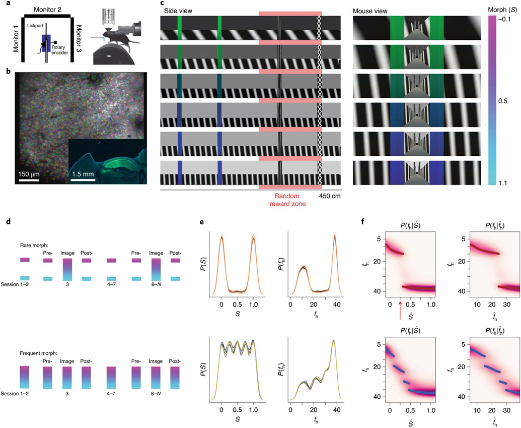
To examine how prior experience affects remapping of hippocampal representations, we performed two-photon imaging of GCaMP in CA1 pyramidal cells as mice traversed visually similar VR linear tracks, which were presented with different frequencies (Fig. 1a,b). In each session, we were able to simultaneously image up to several thousands (range of 161–3,657) of putative CA1 pyramidal cells (Fig. 1b and Extended Data Fig. 1a,b). Note that for the purpose of this study, we define prior experience as the relative frequency with which the mouse encountered different VR stimuli (described below). A trial began with the mouse running in a dark virtual corridor before entering the environment. Once in the environment, the mouse was required to lick for a liquid reward at a visual cue randomly located on the back half of the track (Fig. 1c and Extended Data Fig. 1c-g). Inspired by previous remapping studies that used gradually deformable two-dimensional (2D) environments3,5,10, we designed the VR track such that three dominant visual features of the environment could gradually blend (that is, morph) between two extremes. Visual features included the orientation and frequency of sheared sine waves on the wall, the background color and the color of tower landmarks (Extended Data Fig. 2a-g). The degree of blending in each feature was the coefficient of an affine combination of two values of that stimulus, referred to as the ‘morph value’, S(Sf1 + (1 − S)f2, where f1 and f2 are the two values of the stimulus; Fig. 1c). For each trial, a shared morph value, , was chosen for all features from one of five values (0, 0.25, 0.5, 0.75 and 1.0), and a jitter (uniformly distributed between −0.1 and 0.1) was independently added to each feature. At the end of the track, the mouse was immediately teleported back to the dark corridor to begin a new trial (Supplementary Video 1). For each trial, the morph values of the stimuli were fixed. Across trials, morph values were randomly interleaved according to the training condition (‘rare morph’ or ‘frequent morph’; described below).
Fig. 1 ∣. VR setup for imaging CA1 neurons and the construction of priors for rare morph versus frequent morph conditions.
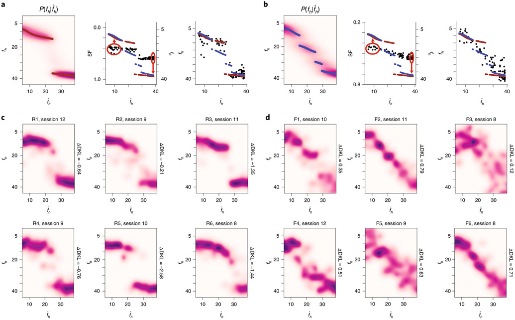
a, Top view (left) and side view (right) of the VR setup, b, Example FOV from an imaging session (mouse F2, session 12; λ = 920 nm) with identified CA1 neurons highlighted (n = 2,006 cells). Inset shows coronal histology for the same animal (green, GCaMP; blue, DAPI (4,6-diamidino-2-phenylindole)). c, The stimulus desig,n with example linear tracks for different morph (S) values (the color bar on the far right indicates S value). Left: side view of VR tracks; the red bar indicates a random reward zone (250–400 cm). Right: view from the perspective of the mouse. d, Illustration of the training protocol for the rare morph (top; n = 6 mice, R1–R6) and the frequent morph (bottom; n = 6 mice, F1–F6) conditions. Imaging was performed on sessions 1, 3 and 8–N (Extended Data Fig. 2f,g). For the rare morph condition, only extreme morph values were shown during trials before imaging begins (pre-) and after imaging ends (post-). For the frequent morph condition, intermediate morph values were shown on each session. Note that for a given trial, morph values were randomly interleaved according to the training condition, e, Left: the empirical prior distribution over the morph values, P(S), at the beginning of session 8 for mice in the rare morph group (top; R1–R6) and the frequent morph group (bottom; F1–F6). Colors indicate mouse ID. Right: same as the left, but after converting morph values to horizontal wall frequency fh (cycles per 500 cm). f, Heatmap of the probability mass function of the posterior probability for each value of (left) and (right). MAP estimates are plotted as maroon (rare; top) or blue (frequent; bottom) points. Note that if CA1 population activity approximates this form of probabilistic inference, the population activity in the rare morph condition will change abruptly when S is between 0.25 and 0.5 (as indicated by the red arrow). Rare morph and frequent morph activity could appear largely similar outside this range of stimuli.
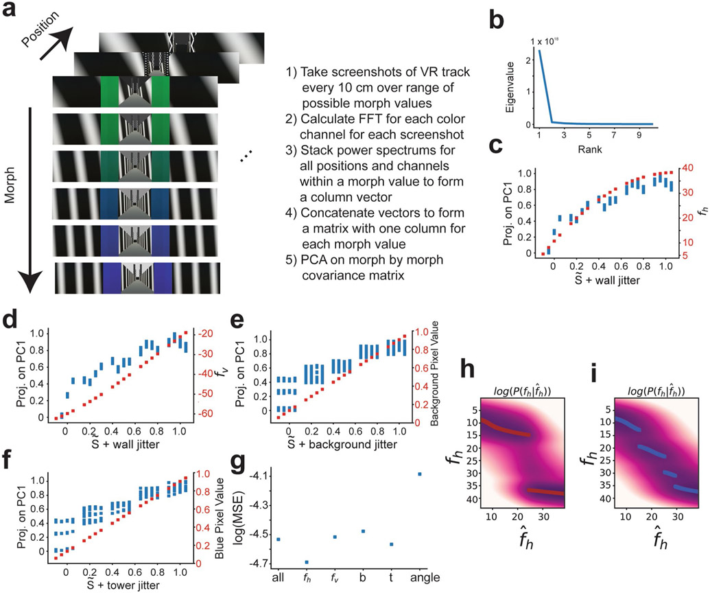
While multiple correlated latent visual dimensions defined the environmental context, the aspect of the stimulus that explained the most variance in the VR environments was the horizontal component of the frequency of the sine waves on the walls (fh). This feature had a monotonic but nonlinear relationship to S (Extended Data Fig. 2a-g). To simplify analyses, we leveraged this fact and defined the overall morph value of a trial on the basis of the wall cues alone (the sum of the shared morph value and the jitter of the wall stimuli such that S = −0.1 to 1.1). We considered two training conditions. In the rare morph condition (n = 6 mice, R1–R6), mice experienced very few trials with intermediate morph values (shared ) during the first 7 training sessions (<4% of trials with intermediate morph values before session 8; Fig. 1d), giving these animals a bimodal prior over S and fh (Fig. 1e and Methods). By contrast, in the frequent morph condition (n = 6 mice, F1–F6), mice were frequently exposed to trials with intermediate morph values (60% of trials with intermediate morph values before session 8; Fig. 1d), giving these animals a comparatively flat prior over S values and a ramping prior over fh values (Fig. 1e).
Under these priors, an observer performing probabilistic inference would make different predictions about the value of intermediate stimuli. For an ideal observer, the probability estimate of the true value of the stimulus, fh, given a noisy observation, , is determined by the posterior distribution: where is the likelihood distribution, which is governed by sensory noise, and P(fh) is the experimentally manipulated prior distribution (the rare morph or frequent morph condition). In the rare morph condition, the posterior distribution maintains two modes of high probability close to the extreme values of the stimulus (log posterior; Fig. 1f and Extended Data Fig. 2h). In the frequent morph condition, the posterior distribution shifts the density gradually from one extreme value of fh to the other (log posterior; Fig. 1f and Extended Data Fig. 2i). Importantly, if the CA1 population activity approximates this form of probabilistic inference, the population activity in the rare morph condition will abruptly change when S is between 0.25 and 0.5 (as indicated by the red arrow in Fig. 1f), while the population activity in the frequent morph condition will gradually change across S values, with the rate of change being the highest when S is less than 0.5 (see Extended Data Fig. 3 for simulations of these predicted changes).
Prior experience of stimulus frequency determines CA1 place cell remapping.
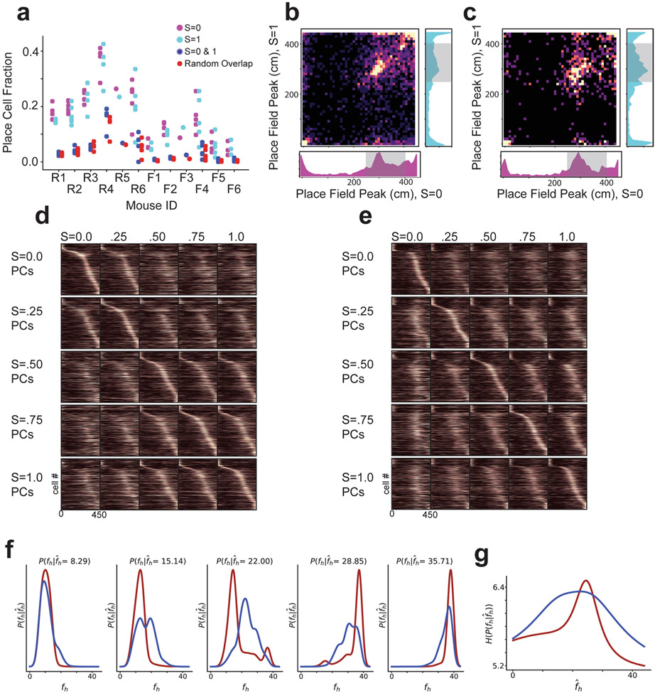
We analyzed CA1 remapping in sessions 8–N, as animals had 7 sessions to develop a stable prior for the frequency of different stimuli. In both the frequent morph and rare morph conditions, large numbers of place cells tiled the track with their place fields (rare = 15,829 place cells across all values, 43% of recorded population, 23% of cells place cells, 21% of cells place cells; frequent = 8,933 place cells across all values, 30% of recorded population, 11% of cells place cells, 10% of cells place cells). The proportion of recorded cells that were classified as place cells was smaller in the frequent morph compared to the rare morph condition (Extended Data Fig. 4a). Under a probabilistic inference framework, this observation could be explained by the increased entropy in the frequent morph posterior compared to the rare morph posterior (that is, the frequent morph posterior is flatter than the rare morph posterior) (Fig. 1f and Extended Data Fig. 4f,g). In other words, the mouse will have greater uncertainty as to which environment it is in for the frequent morph compared to the rare morph condition. This increased entropy (that is, uncertainty) results in more variable population activity, lower spatial information and, therefore, a lower fraction of cells classified as place cells.
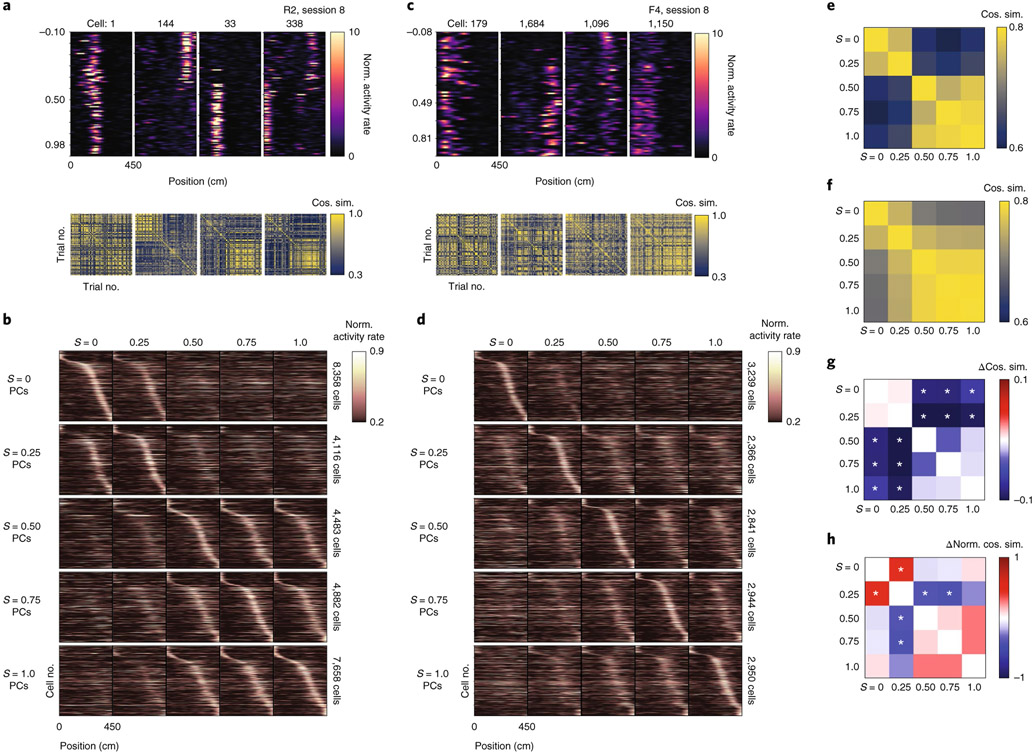
For environments at the extreme morph values ( and ), the proportion of cells with a place field in both environments slightly exceeded the proportion expected by the overlap of independently chosen random populations (P( place cell, place cell) = P( place cell)P( place cell)). Specifically, 6.07% and 1.98% of recorded cells had significant spatial information in both environments for rare morph and frequent morph sessions, respectively (chance 4.78% and 1.06%, respectively; one-sample two-sided t-test of actual minus chance overlap, t=−4.87, P = 1.37×10⁻⁵, N = 45 sessions pooled across all mice) (Extended Data Fig. 4a). Cells with place fields in both extreme environments tended to cluster at the end points of the track and the reward zone (Extended Data Fig. 4b,c). This low degree of overlap suggests that the place representations between the environments at the extreme morph values were largely independent for both the frequent morph and rare morph conditions (that is, global remapping11). Consistent with the probabilistic inference framework introduced above, the transition between these two representations differed between the rare morph and frequent morph conditions. In the rare morph condition, place cells maintained their representation until a threshold morph value (S ≈ 0.25–0.50) and then coherently switched to a different representation (Fig. 2a,b and Extended Data Fig. 4d). However, in the frequent morph condition, place cells gradually changed their representation across intermediate morph values (Fig. 2c,d and Extended Data Fig. 4e). This difference between conditions was also apparent in the normalized place cell population similarity matrices (P < 0.0011, two-sided permutation test using animal identities (IDs), n = 12 mice) (Fig. 2e-h and Methods). These results show at the level of individual place cells that the set of place cells that are most active on a given trial is determined by which environment is most likely given the experience of the animal.
Fig. 2 ∣. Prior experience of stimulus frequency determines CA1 place cell remapping.
a, Top row: co-recorded place cells from an example rare morph session (mouse R2, session 8). Columns show heatmaps from different cells, with each row indicating the activity of that cell on a single trial as a function of the position of the mouse on the VR track (n = 120 trials). Rows are sorted by increasing morph value. The color indicates the deconvolved activity rate normalized by the overall mean activity rate for the cell (Norm. activity rate). Bottom row: trial-by-trial cosine similarity (Cos. sim.) matrices for the corresponding cell above, color coded for maximum (yellow) and minimum (blue) values. b, First row: for all rare morph sessions 8–N, place cells (PCs) were identified in the morph trials and sorted by their location of peak activity on odd-numbered trials. The average activity on even-numbered trials is then plotted (left-most panel). Each row indicates the activity rate of a single cell as a function of position, averaged over even-numbered morph trials. The color indicates the activity rate normalized by the peak rate from the odd-numbered average activity rate map for that cell. The trial-averaged activity rate map for these cells is then plotted for the other binned morph values using the same sorting and normalization process (remaining panels to the right). Second to fifth rows: same as the top row for the same rare morph sessions, but for place cells identified in the (second row), (third row), (fourth row) and (fifth row) morph trials. For each row, cells are sorted and normalized across all panels according to the place cells identified in the respective morph trial, c, Same as in a, but for an example frequent morph session (mouse F4, session 8, n = 75 trials). d, Same as in b, but for all frequent morph sessions 8–N. e, Average cosine similarity matrix for the union of all rare morph place cells in b. f, Average cosine similarity matrix for the union of all frequent morph cells in d. g, Rare morph cosine similarity matrix, from e, minus the frequent morph cosine similarity matrix from f (asterisks indicate significance based on a permutation test of mice across conditions, P < 0.05, two-sided). h, Same as g, but the cosine similarity matrix for each cell is z-scored before group comparisons (asterisks indicate significance based on a permutation test of mice across conditions, P < 0.0011, two-sided).
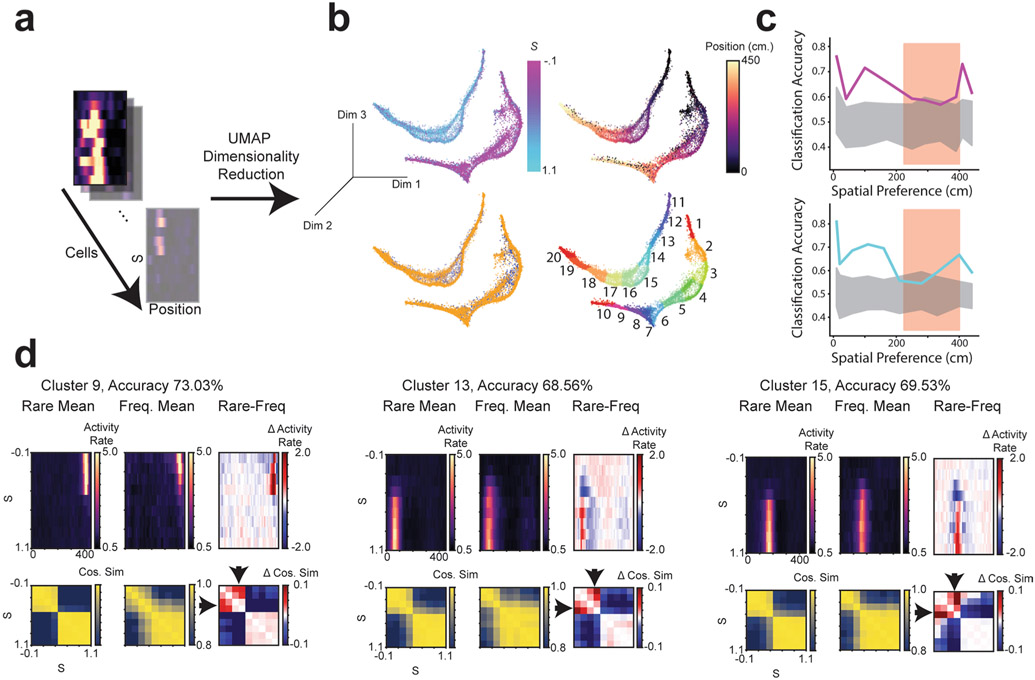
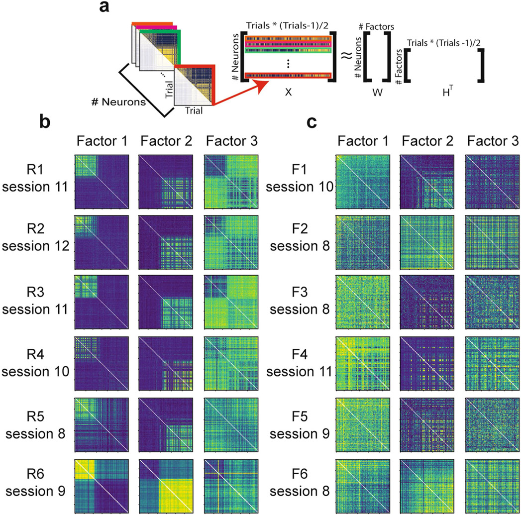
Two unsupervised approaches confirmed that the remapping patterns we observed in place cells reflected the dominant patterns of activity in the greater CA1 population of both place and non-place cells. First, we performed nonlinear dimensionality reduction using uniform manifold approximation and projection (UMAP)14 (Extended Data Fig. 5 and Methods). This approach independently identified spatially selective and context-specific cells. Rare and frequent morph cells were also separable using this approach. As in our other analyses, UMAP showed that cells from the rare morph condition maintained a spatial representation until a threshold morph value (S ≈ 0.25–0.5), while cells from the frequent morph condition gradually changed their position, modulated activity across morph values and had wider spatial preferences (Extended Data Fig. 5). These findings were also confirmed using a second unsupervised approach: non-negative matrix factorization (Extended Data Fig. 6).
Population similarity analyses reveal distinct remapping patterns visible at the level of single trials.
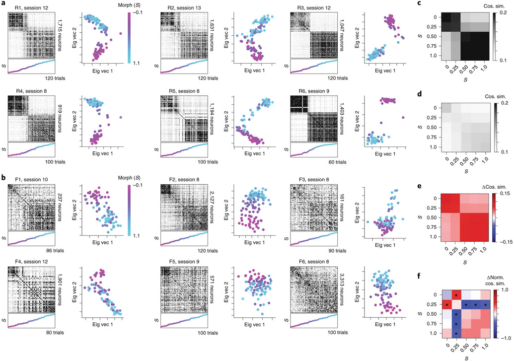
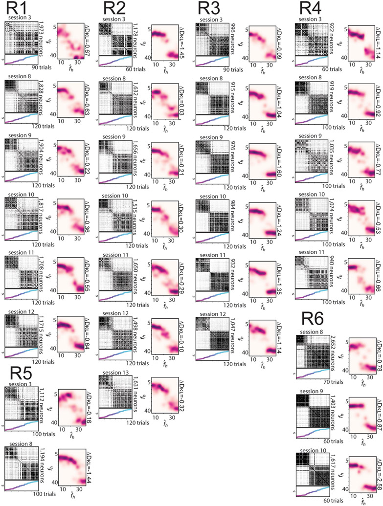
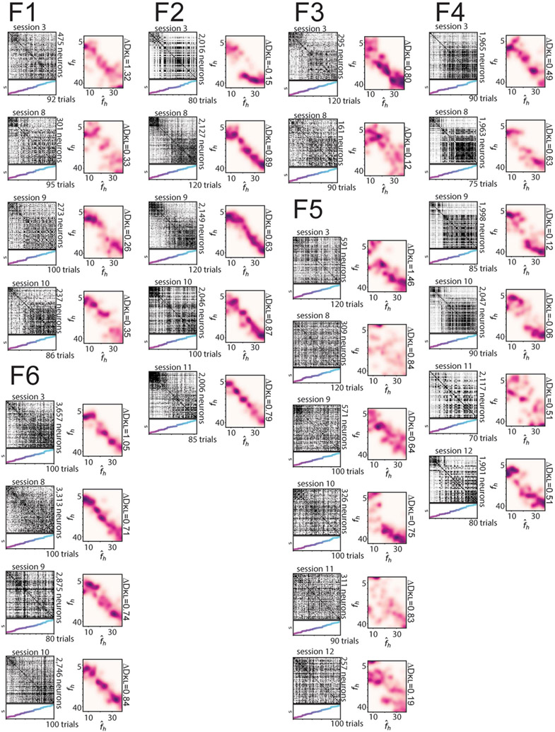
To more closely compare the CA1 population activity and the posterior inference of the context, we next investigated neural activity within a given session. Trial-by-trial population similarity matrices for individual sessions yielded results consistent with those observed above and consistent with our model of a neural posterior distribution (Extended Data Fig. 3). For the rare morph condition, a strong block diagonal structure in the trial-by-trial similarity matrices suggested clustering of morph values into two representations (Fig. 3a). Occasionally, we observed that trials near the threshold for switching between these two blocks would randomly take on one extreme representation or the other. For example, checker-board dark bands were observed in the similarity matrices near , as if the matrix was missorted for R1 session 8, R2 session 13, R3 session 9, R4 session 11, R5 session 8 and R6 session 10 (Extended Data Fig. 7). This suggests that the neural population may perform a computation equivalent to sampling values from the posterior distribution, as the rare morph posterior has two modes of similar probability at these intermediate values of fh (Extended Data Fig. 2h) and the neural representation could randomly take on a representation for either of these modes. In the frequent morph condition, the trial-by-trial similarity matrices showed a gradual transition between the two extreme morph values (Fig. 3b). The greater visual heterogeneity of the frequent morph similarity matrices is also consistent with the idea that the population is representing samples from the multimodal high entropy frequent morph posterior. Strikingly, the neural activity patterns observed in the rare morph and frequent morph conditions were highly consistent across individual mice (Fig. 3) and across all sessions in all mice (Extended Data Figs. 7 and 8). As predicted, group differences in trial-by-trial similarity were significant for trials after z-scoring within session similarity (P < 0.05 two-sided mouse permutation test, n = 12 mice) (Fig. 3c-f and Methods).
Fig. 3 ∣. Population similarity analyses reveal distinct remapping patterns visible at the level of single trials.
a, Data for an example session from each mouse in the rare morph condition. The left panels show population trial-by-trial cosine similarity matrices for example rare morph sessions, color coded for maximum (black) and minimum (white) values. The number of cells imaged in the example sessions is denoted on the right. The color and the height on the vertical axis of the scatterplots below indicate the morph value, with trials sorted in ascending morph value as indicated by the color bar. Note that this is not the order in which trials were presented. The right panels show projections of the activity of each trial onto the principal two eigenvectors (Eig vec 1 and 2) of the similarity matrix. Each dot indicates one trial, colored by morph value. b, Same as in a, but for an example session from each mouse in the frequent morph condition. All individual sessions from all mice are shown in Extended Data Figs. 7 and 8. c, Population similarity matrices were binned across morph values (diagonal entries of the original matrix excluded) and averaged across sessions within animals and then across animals for all rare morph sessions 8–N (R1–R6 mice, n = 24 sessions). d, Same as c, but for all frequent morph sessions 8–N (F1–F6 mice, n = 21 sessions). e, The difference between the average rare morph and frequent morph (c) trial-by-trial similarity matrices. f, Same as e, but after the binned trial-by-trial similarity matrix for each session is z-scored (asterisks indicate significant differences, P < 0.05, mouse permutation test, two-sided).
CA1 representations show stable discrimination of morph values along the length of the track.
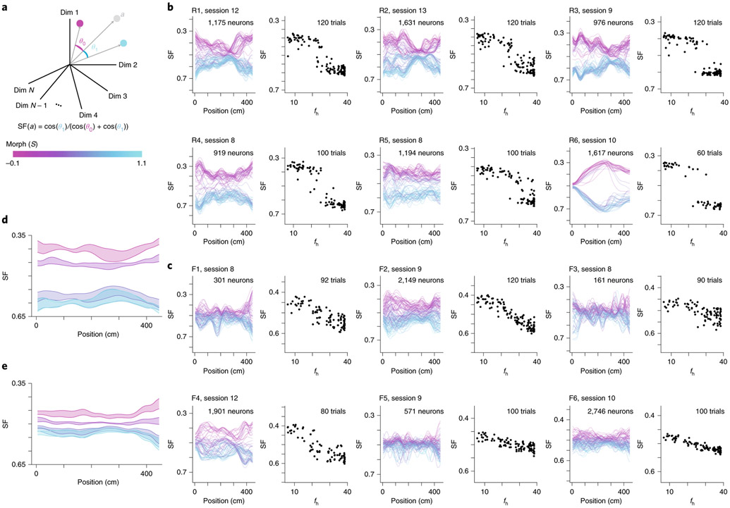
We then asked how similar the CA1 neural representations for single trials were to the average CA1 neural representation for and morph values. To quantify this, we defined a similarity fraction (SF) between the average activity for and trials. This value is the ratio of the population vector similarity to the centroid (average of the position binned activity rate across trials) to the sum of similarities to the and centroids (Fig. 4a). Values less than 0.5 indicate trials relatively closer to the centroid, while values above 0.5 indicate trials relatively closer to the centroid. Plotting SF as a function of the position of the animal along the VR track revealed a clustering of stable representations across the entire length of the track for the rare morph condition (Fig. 4b,d) and a spectrum of representations for the frequent morph condition (Fig. 4c,f). Consequently, we calculated a summary SF value for each trial and considered it as a function of morph value (SF(S) or SF(fh); Fig. 4b,c). Again, these observations were highly consistent across individual mice (Fig. 4b,c). Together, these results indicate that remapping rapidly occurred after the start of a new trial and remained stable as the animal traversed the virtual track. Examining the SF(fh) plots for example sessions (right panels in Fig. 4b,c), we noted that these plots resembled noisy versions of the maximum a posteriori (MAP) estimates from the rare morph and frequent morph posterior distributions. Rare morph SF(fh) values gradually increased at smaller values of fh until a threshold, and then jumped to a higher value and remained essentially constant for higher fh values. Frequent morph SF(fh) values gradually increased over most of the range of fh values and remained stable at high values of fh.
Fig. 4 ∣. CA1 representations show stable discrimination of morph values along the length of the track.
a, Schematic of how the SF is calculated. Each dimension indicates the activity of a single neuron at a single position bin. For the left panels in b and c, only one position bin is included in the calculation at a time. The centroid is calculated by averaging the population vector for all trials (magenta dot). Likewise, the centroid is calculated by averaging the vector for all trials (cyan dot). b, Data for an example session from all mice in the rare morph condition. Left panels show the SF plotted as a function of the position of the animal on the track for each trial in an example rare morph session (for example, mouse R3, session 9; 976 cells, 120 trials). Each line represents a single trial, and the color code indicates the morph value (color bar in a). Right panels show the SF(fh) plotted (black dots, left vertical axis) as a function of fh for the same example session shown on the left. Each dot represents a single trial, c, Same as b, but for an example session from all mice in the frequent morph condition. All individual sessions from all are mice shown in Extended Data Figs. 7 and 8. d, Average SF by position plot across rare morph sessions (8–N) and animals (R1–R6). Shaded regions represent across-animal means for binned morph values (, 0.25, 0.50, 0.75 and 1.0) ± s.e.m. across mice. Note that the data for morph values 0.75 and 1.0 are nearly overlapping, e, Same as d, but for all frequent morph sessions (8–N, F1–F6 mice, n = 19 sessions). Note that the data for morph values 0.5, 0.75 and 1.0 are partially overlapping.
CA1 population activity approximates optimal estimation of the stimulus.
The above observation suggested that we could form an approximation of the posterior distribution, Q, by simply stretching and shifting the summary SF(fh) curve to be in the range of the maximuum a posteriori (MAP) estimates via an affine function. That is, . We formed Q estimates independently for each session. We chose the parameters of the affine function such that the median of SF () values was equal to the average of the rare morph and frequent morph MAP estimates for SF () trials, and the median of the SF () values was equal to the average of the rare morph and frequent morph MAP estimates for SF () trials (Fig. 5a,b). Note that the MAP estimates are nearly identical for the rare and frequent morph conditions at these values of the the stimulus. We performed kernel density estimation on the resulting data points to obtain probability distributions.
Fig. 5 ∣. CA1 hippocampal remapping approximates the optimal estimation of the stimulus.
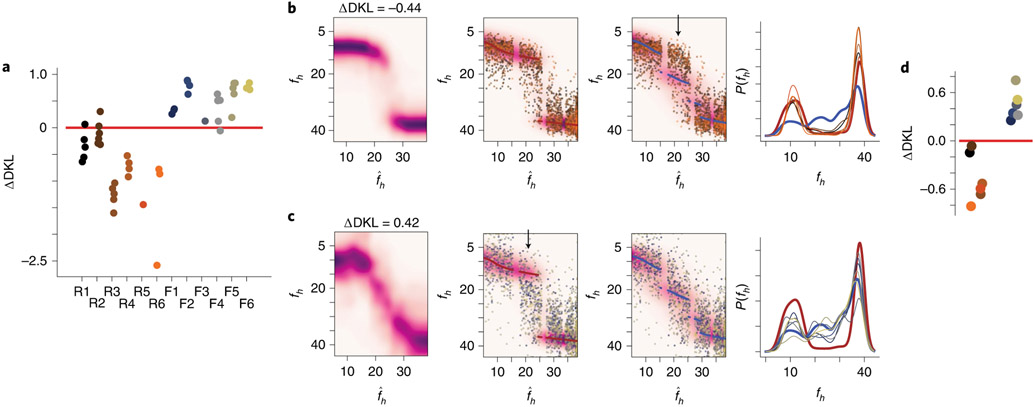
a, Schematic for calculating estimates. Left: ideal posterior distribution for the rare morph prior as in Fig. 1f. Middle: SF(fh) plotted (black dots, left vertical axis) for an example rare morph session (top; R3, session 11; 932 cells, 120 trials). The MAP estimates as a function of fh are plotted for the rare morph (maroon dots, right vertical axis) and frequent morph (blue dots, right vertical axis) conditions. The red circled regions indicate the and trials used to estimate the affine transform for forming Q estimates. Right: example from the middle column after affine transform. To perform the affine transform, we stretched and shifted the range of SF(fh) values (black dots) in the direction of the red arrows (middle panel) to match the range of the MAP estimates as a function fh (maroon dots for the rare morph condition or blue dots for the frequent morph condition). Q estimates were then formed by kernel density estimation. b, Same as a, but for the ideal posterior distribution for the frequent morph prior (left) and an example frequent morph session (F2, session 11; 2,006 cells, 85 trials). c, Q estimates for an example session from each mouse in the rare morph condition. d, Same as c, but for an example session from each mouse in the frequent morph condition. All individual sessions from all mice are shown in Extended Data Figs. 7 and 8.
Q estimates derived from single sessions bore clear resemblance to the ideal posterior distributions (Fig. 5c,d, with all sessions shown in Extended Data Figs. 7 and 8). We then measured the relative distance (ΔDKL, a difference in Kullback–Leibler divergences) of the Q estimate for each session to either the ideal rare morph or frequent morph posterior (Fig. 6a and Methods). Each ΔDKL is akin to a hypothesis test, whereby a negative ΔDKL value indicates the session Q estimate is closer to the rare morph posterior, while a positive ΔDKL value indicates it is closer to the frequent morph posterior. This ΔDKL measure took the expected sign (rare sessions ΔDKL < 0 and frequent sessions ΔDKL > 0) in 41 out of 45 sessions, and it took the expected sign in every session from 9 out of 12 mice (across animal mean±s.e.m.: rare ΔDKL = −0.88 ± 0.23, frequent ΔDKL = 0.50±0.11; P<0.0011, two-sided animal permutation test, n = 12 mice) (Methods). Combining data from all sessions and all mice gave a robust approximation (ΔDKL) of the posterior for both the rare morph and frequent morph conditions (rare ΔDKL = −0.44, frequent ΔDKL = 0.42; left-most panels of Fig. 6b,c). To further visualize the consistency of this result, we plotted the linearly transformed SF(fh) values on top of the ideal rare morph and frequent morph posteriors (middle two panels of Fig. 6b,c). The data clouds showed a clear overlap with the appropriate posterior. A clear conflict with the posterior for the opposite condition was seen for trials (; locations of mismatch highlighted with black arrows in Fig. 6b,c). Using the accumulated approximation of the posterior over all sessions, we were able to reconstruct the prior, P(fh), for each mouse in an unsupervised manner with high accuracy (right-most panels of Fig. 6b,c). A similar ΔDKL metric showed that the reconstructed priors are closer to the ideal prior from the correct condition than the ideal prior from the incorrect condition (Fig. 6d) (across animal mean±s.e.m.: rare ΔDKL = −0.46 ± 0.12, frequent ΔDKL = 0.46±0.07; P<0.0011, animal permutation test, n = 12 mice). Thus, looking only at the neural activity, we could reproduce the posterior distributions of the animal and predict the relative frequency with which the mice saw the different VR environments.
Fig. 6 ∣. Individual animal prior distributions can be recovered solely from remapping patterns.
a, Relative distances of the Q estimates for each session to the ideal rare morph and frequent morph posteriors, ΔDKL. Each dot represents an individual session. The mouse ID is on the horizontal axis. Jitters were added to the horizontal location for visibility. b, Left: Q estimate achieved by averaging and re-normalizing the across-session Q estimate for each mouse. Middle left: the background heatmap is the ideal rare morph posterior distribution. The maroon scatterplot points are the MAP estimate from this ideal posterior. The remaining points are the linearly transformed SF(fh) values (as in Fig. 5a, rightmost panel) for every trial and every mouse (n = 2,610 trials). Colors indicate the mouse ID. Middle right: same transformed SF data as in the middle left, but plotted with the ideal frequent morph posterior (heatmap) and MAP estimates (blue scatterplot). The black arrow indicates a mismatch between the transformed SF(fh) values and the ideal posterior. Right: ideal rare morph prior distribution (maroon), ideal frequent morph prior distribution (blue) and the reconstructed prior for each rare morph mouse (colors indicate mouse the ID). Note that this is the unsupervised recovery of the priors. c, Same as b, but for accumulated data from all mice in the frequent morph group (n = 1,986 trials). d, Relative distances of reconstructed priors (left: rare morph mice; right: frequent morph mice) to either ideal prior, ΔDKL.
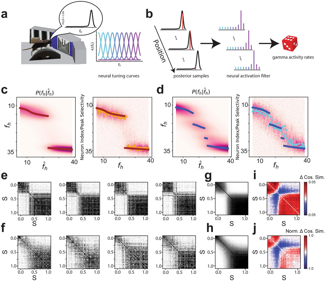
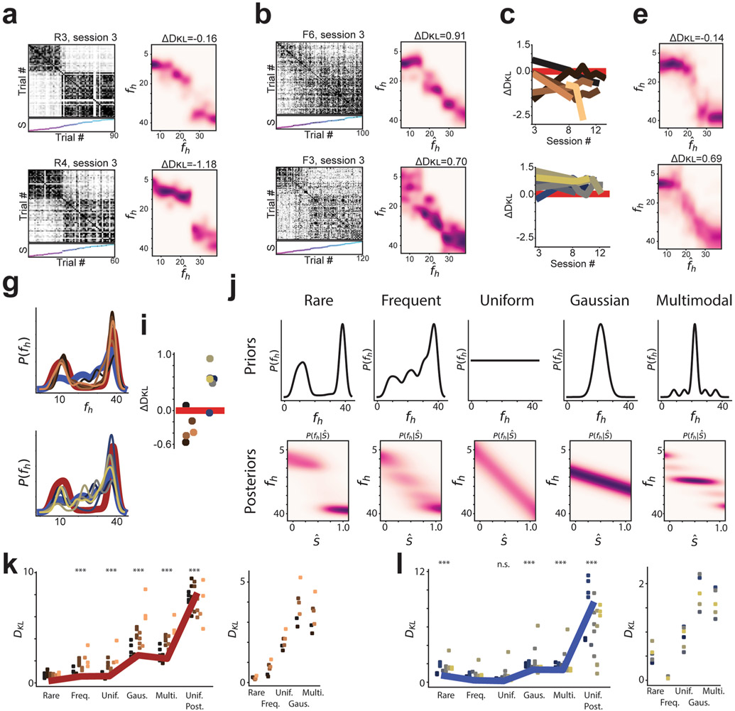
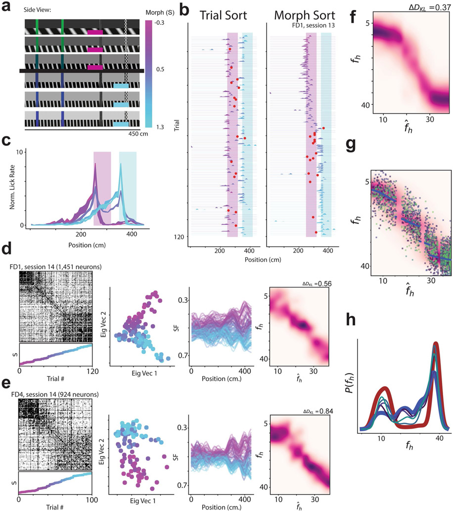
Of note, these remapping patterns observed in rare morph versus frequent morph conditions were stable over sessions and emerged early in training in most animals (Extended Data Figure 9a-g). Furthermore, a comparison of Q estimates to a number of other null model posteriors yielded poor fits to the data (Extended Data Fig. 9j-l). In an additional set of experiments, we trained frequent morph mice to discriminate between morph values greater than 0.5 versus less than 0.5 and report their decision by licking in different spatial locations on the VR track. The remapping patterns were similar to those observed in frequent morph mice that did not perform this task (Extended Data Fig. 10). Simulating neural populations that were designed to stochastically encode the posterior distributions also reproduced the remapping patterns described above (Extended Data Fig. 3).
Simple associative-learning mechanisms can approximate probabilistic inference in neural populations.
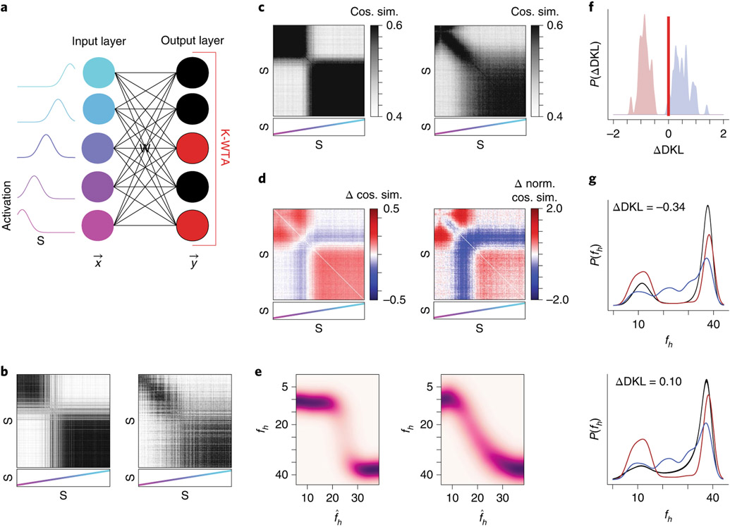
Finally, we sought to implement a network model capable of learning approximate probabilistic inference. We reproduced key experimental findings by implementing a model with the following three main components: (1) stimulus-driven input to all cells, (2) Hebbian learning by cells on these inputs and (3) competition between neurons via a K-winners-take-all (KWTA) mechanism15,16 (Fig. 7a). Using identical model parameters, we simulated learning under the rare morph and frequent morph conditions by drawing stimuli from the corresponding priors. Model-derived trial-by-trial similarity matrices (Fig. 7b—d) bore a clear resemblance to those derived from experimental data (Fig. 7a,b), and model-derived SF values and Q estimates were good matches to the appropriate posterior distributions (Fig. 7e,f). As in the analyses above, we could accurately reconstruct the prior distributions from the Q estimates (Fig. 7g). These unsupervised reconstructions were quantitatively more similar to the prior of the matching condition, but the match between the reconstruction and the true priors was not as compelling as the match seen in the neural data. This model has the strength of approximating a normative solution to hidden-state inference with a biologically plausible unsupervised learning rule and a simple architecture17-19.
Fig. 7 ∣. Neural context discrimination is well explained by associative-learning models.
a, Schematic of the computational model. The input layer contains neurons that form a basis for representing the stimulus using radial basis functions. Activations are linearly combined via the matrix W, and thresholding is applied to the output layer via a KWTA mechanism to achieve the output activation. W is updated after each stimulus presentation using Hebbian learning. Model training is performed by drawing trials randomly from either the rare morph prior or the frequent morph prior. b, Left: trial-by-trial similarity matrix, as in Fig. 3a, for an example model trained under the rare morph condition. Right: same as the left, but for an example model trained under the frequent morph condition. c, Average trial-by-trial similarity matrices across model instantiations (n = 50) for rare morph (left) and frequent morph (right) trained models. d, Left: the average rare morph similarity matrix minus the average frequent morph similarity matrix. Right: same as the left, but the similarity matrix for each model is z-scored before averaging. e, Q estimates for accumulated rare morph trained models (left) and frequent morph models (right). f, Smoothed histogram of ΔDKL values for rare morph (maroon) and frequent morph (blue) trained models. Red line indicates zero. g, Reconstructed priors for rare morph (top, black, mean ±s.e.m.) and frequent morph (bottom, black, mean ±s.e.m.) trained models. Note that this is the unsupervised recovery of the priors. Ideal rare morph (maroon) and frequent morph (blue) priors are shown for reference. ΔDKL is for the averaged reconstructed prior.
Discussion
We showed that remapping patterns in the CA1 can be precisely predicted by the prior experience of the animal, with the hippocampus approximating an ideal combination of these prior beliefs with information about the current stimulus. This framework provides a unifying explanation for earlier works using morphed 2D environments, which resulted in conflicting findings regarding whether CA1 place cells followed discontinuous or continuous remapping patterns3,5,10. Due to the nature of the previous morph experiments, it is difficult to exactly quantify the sensory experience of the animals in the morphed environment; however, making reasonable assumptions, we reproduced each of the conflicting findings from previous studies using our probabilistic inference framework (Supplementary Figs. 1-4). In studies that, during training, used multimodal cues to define the extremes of the environment10 (simulated replication in Supplementary Fig. 1) or placed the extreme environments in different locations3 (simulated replication in Supplementary Fig. 2), the modes of the prior of the animal were likely distinct, leading to discrete remapping patterns similar to what we observed in the rare morph condition. In studies that, during training, did not make the extremes of the environment as distinct5 (simulated replication in Supplementary Fig. 3) or placed the extreme environments in the same physical location3 (simulated replication in Supplementary Fig. 4), the modes of the prior of the animal were likely more overlapping, leading to gradual remapping patterns similar to what we observed in the frequent morph condition13. Here, we explicitly demonstrated that CA1 representations can follow either discontinuous or continuous remapping patterns, with the remapping pattern observed quantitively predicted by the prior experience of the animal. It remains to be seen whether these dynamics emerge in CA1 or whether they are inherited from an earlier stage of processing, although previous work points to the CA3 region of the hippocampus and the dentate gyrus as important inputs for CA1 rate remapping20.
Previous works generally classified hippocampal place cell remapping as either rate remapping (in which the firing rate of place fields differ) or global remapping (in which place fields turn on/off or move spatial locations such that the activity patterns of place cells are uncorrelated)5,6,8. Here, in both rare morph and frequent morph conditions, the remapping we observed more closely matches the definition of global remapping. While in previous work, global remapping has often been observed when an animal moves between two discrete environments, in our experiments, we did not examine the impact of novel environments with highly non-overlapping sensory cues. However, the framework used to predict remapping patterns in the current work predicts that if an environment has little sensory cue overlap with previously experienced environments, the probability of being in one of these previously experienced environments is very low and therefore discrete remapping patterns, similar to those observed in the rare morph condition, would be observed. This is generally consistent with previous observations that small changes in the sensory cues associated with an environment result in rate remapping, while large changes in the sensory cues associated with an environment result in global remapping. One possibility for future work to consider is that if the probability of being in a previous familiar environment is sufficiently low, a novelty detection mechanism (for example, activation of supramammilary nucleus inputs to hippocampal dentate gyrus cells21) triggers the formation of a new map (see also ref. 13).
While the experiments described here were performed in head-fixed mice navigating VR environments, we would expect to observe the same influence of prior experience on CA1 remapping patterns in freely moving animals22. Multiple studies have reported that hippocampal remapping in VR scenarios shows many of the same features as remapping in freely moving animals, including the fraction of place cells active between distinct environmental contexts and the timescale of remapping23-27. VR has also been a useful paradigm to examine latent encoding features of hippocampal cells that are not apparent in freely moving animals, such as CA1 neurons that show directional coding and selectivity for distance traveled28,29. While we did not specifically consider these coding features of CA1 neurons, the observation that both CA1 place and non-place cells follow identical remapping patterns points to the influence of prior experience on CA1 remapping dynamics as a general coding feature of the entire CA1 neuronal population. The idea that prior experience is a general coding feature of the CA1 is also consistent with our computational model (Fig. 7), which showed that this type of coding can be accomplished with generic circuit components and learning mechanisms.
Our computational model demonstrated that our experimental results agree with associative-learning mechanisms in the hippocampus, a long-standing proposal for how the hippocampus implements memory16,30-32. Moreover, the results reported here broadly complement the recently proposed probabilistic framework of a successor-like representation in the hippocampus and provide a potential mechanism for switching between successor representations for different contexts13,33. The remapping patterns described here also intersect with frameworks that use attractor dynamics34,35, which can perform Bayesian state estimation36,37, an idea that could be explored in future work. Our findings also build on the emerging idea that the hippocampal–entorhinal circuit represents not only the location of the animal in physical space but also its location along relevant non-spatial stimulus dimensions38,39. In our experiments, CA1 cells systematically varied their activity as a function of position in response to changes in the visual features of virtual environments. These population dynamics were strongly influenced by the prior experience of the animal, which allowed the circuit to approximate the optimal estimate of the identity of the context based on the latent visual dimensions of the environment.
Methods
Subjects.
All procedures were approved by the Institutional Animal Care and Use Committee at Stanford University School of Medicine. Male and female (n = 9 male, 7 female) mice were housed in groups of between one and five same-sex littermates. After surgical implantation, mice were housed in transparent cages with a running wheel and kept on a 12-h light–dark schedule. All experiments were conducted during the light phase. Mice were between 2 and 5 months at the time of surgery (weighing 18.6–29.8 g). Before surgery, animals had ad libitum access to food and water. Mice were excluded from the study if they failed to perform the behavioral task described below or the quality of the calcium imaging was insufficient (for example, low levels of indicator expression, many nuclei filled with GCaMP, overexpression-induced ictal activity or cell death). See the Nature Research Reporting Summary for more details.
Statistics.
In most instances, we attempted to avoid inappropriate assumptions about data distributions by using nonparametric permutation tests. These tests are described in detail in the later sections of the Methods. Place cell significance tests are described in “Place cell identification and plotting” Across-animal permutation tests are described in “Place cell similarity matrices”, “Population trial-by-trial similarity matrices”, “Estimating posterior distributions from population activity (Q estimates)” and “Reconstructing prior distributions”. Additional permutation tests are described in “UMAP for dimensionality reduction”. Wilcoxon signed-rank tests and t-tests were performed using the SciPy (https://scipy.org/) statistics module. For t-tests, distributions were assumed to be normal, but this was not formally tested. UMAP was performed using the umap-learn package (https://umap-learn.readthedocs.io/en/latest/). Density-based spatial clustering of applications with noise (DBSCAN), non-negative matrix factorization and logistic regression were implemented using Scikit-learn (https://scikit-learn.org/stable/). No statistical methods were used to predetermine the number of mice to include in this study, but our sample sizes were similar to those reported in previous publications23,26,27.
Calcium indicator expression and assignment of animals to experimental groups.
Four methods were used to express GCaMP in CA1 pyramidal cells. (1) For F1–F3, F5 and F6, R4 and R5, and FD1–FD4 mice (Extended Data Fig. 10 only), hemizygous CaMKIIa-cre mice (Jackson Laboratory, stock 005359)40 were first anesthetized by an intraperitoneal injection of a ketamine–xylazine mixture (~85 mg per kg). Then, adeno-associated virus containing cre-inducible GCaMP6f under a ubiquitous promoter (AAV1-CAG-FLEX-GCaMP6f-WPRE; Penn Vector Core) was injected into the left hippocampus (500 nl injected at −1.8 mm anterior–posterior (AP), −1.3 mm medial–lateral (ML), 1.4 mm from the dorsal surface (dorsal–ventral (DV)) using a 36-gauge Hamilton syringe (World Precisions Instruments). The needle was left in place for 15 min to allow for virus diffusion. The needle was then retracted and imaging cannula implantation was performed (described in the section below). (2) For mouse R6, the same procedure as above was performed with a C57BL/6J mouse (Jackson Laboratory, stock 000664) and non-cre inducible jGCaMP7f virus (AAV1-syn-jGCaMP7f-WPRE; AddGene, viral prep 104488-AAV1)41. (3) For R1–R3 mice, hemizygous CaMKIIa-cre mice were maintained under anesthesia via inhalation of a mixture of oxygen and 0.5–2% isoflurane. A retro-orbital injection of AAV-PhP.eB-EF1a-DIO-GCaMP6f (~2.6 × 10¹¹ viral genomes per mouse; Stanford Gene Vector and Virus Core) was performed. This retro-orbital injection occurred 20 days before imaging cannula implantation (described below). (3) Mouse F4 was a transgenic GCaMP animal (Ai94;CaMKIIa-tTA;CaMKIIa-cre, hemizygous for all alleles; Jackson Laboratory, stock 024115) expressing GCaMP6s in all CaMKIIa-positive cells. R1–R3, F1–F3 and FD1–4 mice were run as individual cohorts. All other mice were randomly assigned to experimental groups. Due to the nature of the experiments, blinding the experimenter to the experimental condition of the mouse was not possible.
Imaging cannula and implant procedure.
We modified previously described procedures for imaging CA1 pyramidal cells27,42,43. Imaging cannulas consisted of a 1.3-mm long stainless-steel cannula (3-mm outer diameter, McMaster) glued to a circular cover glass (Warner Instruments, number 0 cover glass, 3 mm in diameter; Norland Optics, number 81 adhesive). Excess glass overhanging the edge of the cannula was shaved off using a diamond-tipped file.
For the imaging cannula implant procedure, animals were anesthetized by an intraperitoneal injection of a ketamine–xylazine mixture (~85 mg per kg). After 1 h, they were maintained under anesthesia via inhalation of a mixture of oxygen and 0.5–1% isoflurane. Before the start of surgery, animals were also subcutaneously administered 0.08 mg dexamethasone, 0.2 mg carprofen and 0.2 mg mannitol. A 3-mm diameter craniotomy was performed over the left posterior cortex (centered at −2 mm AP, −1.8 mm ML). The dura was then gently removed and the overlying cortex was aspirated using a blunt aspiration needle under constant irrigation with sterile artificial cerebrospinal fluid. Excessive bleeding was controlled using gel foam that had been torn into small pieces and soaked in sterile artificial cerebrospinal fluid. Aspiration ceased when the fibers of the external capsule were clearly visible. Once bleeding had stopped, the imaging cannula was lowered into the craniotomy until the coverglass made light contact with the fibers of the external capsule. To make maximal contact with the hippocampus while minimizing distortion of the structure, the cannula was placed at an approximately 15° roll angle relative to the skull of the animal. The cannula was then held in place with cyanoacrylate adhesive. A thin layer of adhesive was also applied to the exposed skull. A number 11 scalpel was used to score the surface of the skull before the craniotomy so that the adhesive had a rougher surface on which to bind. A headplate with a left offset 7-mm diameter beveled window was placed over the secured imaging cannula at a matching 15° angle and cemented in place with Met-a-bond dental acrylic that had been dyed black using India ink.
At the end of the procedure, animals were administered 1 ml of saline and 0.2 mg of Baytril and placed on a warming blanket to recover. Animals were typically active within 20 min and were allowed to recover for several hours before being placed back in their home cage. Mice were monitored for the next several days and given additional carprofen and Baytril if they showed signs of discomfort or infection. Mice were allowed to recover for at least 10 days before beginning water restriction and VR training.
Two-photon imaging.
To image the calcium activity of neurons, we used a resonant-galvo scanning two-photon microscope (Neurolabware). A 920-nm light (Coherent Discovery laser) was used for excitation in all cases. Laser power was controlled using a Pockels cell (Conoptics). The average power for excitation for the AAV1-CAG-FLEX-GCaMP6f-WPRE mice, the AAV1-syn-jGCaMP7f-WPRE mouse and the Ai94;CaMKIIa-tTA;CaMKIIa-cre mouse was 10–40 mW (F1–6, R4–6 and FD1–4). For the AAV-PhP.eB-EF1a-DIO-GCaMP6f mice, the typical laser power was 50–100 mW (R1, R2 and R3). The 1 × 1-mm field of view (FOV) (512 × 796 pixels) was collected using unidirectional scanning at 15.46 Hz. Cells were imaged continuously under constant laser power until the animal completed 60–120 trials, the session exceeded 40 min or the mouse stopped running consistently.
Putative pyramidal cells were identified using the Suite2P software package (https://github.com/MouseLand/suite2p), and the segmentations were curated by hand to remove regions of interest that contained multiple somas or dendrites or contained cells that did not display a visually obvious transient. This method identified between 161 and 3,657 putative pyramidal neurons per session depending on the quality of the imaging window implant and expression of the virus. We did not attempt to follow the same cells over multiple sessions; however, we attempted to return to roughly the same FOV on each session. For all analyses, we used the extracted activity rate obtained by deconvolving the ΔF/F with a canonical calcium kernel. We do not interpret this result as a spike rate. Rather, we view it as a method to remove the asymmetric smoothing on the calcium signal induced by the indicator kinetics.
VR design.
All VR environments were designed and implemented using the Unity game engine (https://unity.com/). Virtual environments were displayed on three 24-inch LCD monitors that surrounded the mouse and were placed at 90° angles relative to each other. A dedicated PC was used to control the virtual environments, and behavioral data were synchronized with calcium-imaging acquisition using TTL pulses sent to the scanning computer on every VR frame. Mice ran on a fixed-axis foam cylinder, and the running activity was monitored using a high precision rotary encoder (Yumo). Separate Arduino Unos were used to monitor the rotary encoder and to control the reward delivery system.
Water restriction and VR training.
To incentivize mice to run, the water intake of the animals was restricted. Water restriction was not implemented until 10–14 days after the imaging cannula implant procedure. Animals were given 0.8–1 ml of 5% sugar water each day until they reached ~85% of their baseline weight and given enough water to maintain this weight.
Mice were handled for 3 days during initial water restriction and fed through a syringe by hand to acclimate them to the experimenter. On the fourth day, we began acclimating animals to head fixation (day 4: ~30 min; day 5: ~1 h). After mice showed signs of being comfortable on the treadmill (walking forward and pausing to groom), we began to teach them to receive water from a lickport. The lickport consisted of a feeding tube (Kent Scientific) connected to a gravity-fed water line with an in-line solenoid valve (Cole Palmer). The solenoid valve was controlled using a transistor circuit and an Arduino Uno. A wire was soldered to the feeding tube, and the capacitance of the feeding tube was sensed using an RC circuit and the Arduino capacitive sensing library. The metal headplate holder was grounded to the same capacitive-sensing circuit to improve signal to noise, and the capacitive sensor was calibrated to detect single licks. The water delivery system was calibrated to deliver ~4 μl of liquid per drop.
After mice were comfortable on the ball, we trained them to progressively run farther distances on a VR training track to receive sugar water rewards. The training track was 450-cm long with black and white checkered walls. A pair of movable towers indicated the next reward location. At the beginning of training, this set of towers were placed 30 cm from the start of the track. If the mouse licked within 25 cm of the towers, it would receive a liquid reward. If the animal passed by the towers without licking, it would receive an automatic reward. After the reward was dispensed, the towers would move forward. If the mouse covered the distance from the start of the track (or the previous reward) to the current reward in under 20 s, the inter-reward distance would increase by 10 cm. If it took the animal longer than 30 s to cover the distance from the previous reward, the inter-reward distance would decrease by 10 cm. The minimum reward distance was set to 30 cm and the maximal reward distance was 450 cm. Once animals consistently ran 450 cm to get a reward within 20 s, the automatic reward was removed and mice had to lick within 25 cm of the reward towers to receive the reward. After the animals consistently requested rewards with licking, we began rare morph or frequent morph training (described below). Training (from first head fixation to the beginning of the rare morph or frequent morph protocols) took 2–4 weeks.
Morphed environments.
For the rare morph and frequent morph condition experiments, trained mice ran down 450-cm virtual tracks to receive sugar-water rewards. These rewards were placed at a random location between 250 and 400 cm down the track. The reward location was indicated by a small white box with a blue star. Animals received a reward if they licked within 25 cm of the box. Once the animals were well trained, they often ran consistently down the first half of the track and began licking as they approached the reward (Extended Data Fig. 1). They typically stopped to consume the reward and ran at a consistent speed to the end of the track. Well-trained mice ran until they received around 0.8–1 ml of liquid (~200 rewards). To increase the number of trials in a session, rewards were omitted on 20% of trials for some sessions. We also noted that omitting rewards on a small number of trials improved licking accuracy (data not shown).
The visual stimuli for the VR track were chosen so that the extremes of the stimulus distributions could be gradually and convincingly morphed together. The tracks did not change in length nor were the location of salient landmarks changed. The following aspects of the stimulus did change: (1) the frequency and orientation of sheared sine waves on the wall (low-frequency, oriented sine waves into high-frequency nearly vertical sine waves); (2) the color of the first two towers (green to blue); and (3) the color of the background of the visual scene (light gray to dark gray). The morph value, S, for each trial is the coefficient of an affine combination between two extreme values of the stimulus (Sf0 + (1 − S)f1). The choice of an affine transform ensures that stimuli gradually changed from one extreme to the other as a function of single parameter, S. On every trial, a shared morph value, , was chosen for all features from one of five values (0, 0.25, 0.5, 0.75 and 1.0), and a jitter was independently applied to the wall, the tower color and the background color. The jitters were uniform random values from −0.1 to 0.1. The horizontal component of the frequency of the sine waves on the wall (fh) had a monotonic but nonlinear relationship to S, and fh was the most predictive aspect of the stimulus for reconstructing the pixels of the VR environment (Extended Data Fig. 1). Thus, we defined the overall morph value of a trial as the sum of the shared morph value and the jitter of the wall stimuli (S = −0.1 to 1.1).
Rare morph condition.
Mice in the rare morph condition group experienced only trials with a shared morph value of or , with the exception of a subset of imaging sessions. Only one session was run per day. For the first two sessions, the animals experienced trials with randomly interleaved or trials. On the third session, before imaging, the animals experienced 30–50 warm-up trials of randomly interleaved or trials. During imaging (60–120 trials, depending on the running speed of the animal), 50% of the trials were , 0.5 or 0.75 trials. The remaining 50% were or trials. After the imaging session, animals continued to run and trials until they received the rest of their water for the day. For the next four sessions (4–7), the animals again only experienced and trials. For session 8 and all subsequent sessions (8–N) the protocol used in the third session was repeated.
Frequent morph condition.
Mice in the frequent morph condition group experienced randomly interleaved or 1.0 trials with equal probability on every session. During imaging sessions, as for the rare morph condition, animals experienced 30–50 warm-up trials before imaging and continued trials after imaging until they received the rest of their water for the day.
Probabilistic inference using rare and frequent morph priors.
Probabilistic inference, for the purposes of this manuscript, refers to the process of estimating the value of a random variable by calculating the posterior distribution via Bayes’ formula. In this case, the posterior describes the probability of the stimulus, fh, given an observation, . We calculated the posterior using .
P(fh) is the prior distribution and describes the frequency of previously seen stimuli. The rare morph and frequent morph conditions were designed to vary this distribution. For our analyses, we calculated the prior for each mouse as the smoothed normalized histogram of previously seen fh or S values. If we let fh,i be the stimulus value on the ith trial, the smoothed histogram can be calculated as where N(s,σ2) is a Gaussian with mean s and variance σ2 and M is the number of trials. The prior, P(fh), is then calculated by normalizing h(fh) to be a valid distribution, . To calculate the across-mouse prior while giving each mouse equal weight, we calculated the average of the individual mouse priors and then normalized again to ensure the result is a valid distribution.
is the likelihood function, which describes observation noise. In all cases, we assumed that this is a Gaussian centered at fh with variance of 8.23 (25% of the range of wall frequencies). With these distributions in hand, we then calculated the posterior as .
Place cell identification and plotting.
Place cells were identified separately in and 1.0 trials using a previously published spatial information (SI)44 metric . Where λj is the average activity rate of a cell in position bin j, λ is the position-averaged activity rate of the cell and pj is the fractional occupancy of bin j. The track was divided into 10-cm bins, giving a total of 45 bins.
To determine the significance of the SI value for a given cell, we created a null distribution for each cell independently using a shuffling procedure. On each shuffling iteration, we circularly permuted the time series of the cell relative to the position trace within each trial and recalculated the SI for the shuffled data. Shuffling was performed 1,000 times for each cell, and only cells that exceeded all 95% of permutations were determined to be significant place cells.
Place cell sequences (Fig. 1h,j) were calculated independently for each value using split-halves cross-validation. The average firing rate maps from odd-numbered trials were used to identify the position of peak activity. The activity of each cell was also normalized using the peak position-binned activity on odd-numbered trials. Cells were sorted by this position, then the average activity on even-numbered trials was plotted. This gave a visual impression of both the reliability of the place cells within a value and the extent to which these sequences were retained across other morph values. For visualization, single-trial activity rate maps (Fig. 1g-j) were smoothed with a 20-cm (2-spatial bin) Gaussian kernel.
Single-cell trial-by-trial similarity matrices.
For each cell, i, we stacked smoothed single-trial activity rate maps (20-cm or 2-spatial bin width Gaussian kernel) to form a matrix, Ai ∈ RT,J. T is the number of trials and J is the number of position bins. Each row was then divided by its l2norm, yielding a new matrix . The single-cell trial-by-trial cosine similarity matrix is then given by .
Place cell similarity matrices.
We considered the union of all cells across all sessions and mice within an experimental condition that were classified as place cells in any of the trial types. For each cell, i, we calculated the average position-binned activity rate map in each of the values and stacked these smoothed activity rate maps (20-cm or 2-spatial bin width Gaussian kernel) to form a matrix: denotes the number of distinct values (5) and J is the number of position bins. To calculate the trial-by-trial cosine similarity matrix for each cell, we again divided each row of by its l2norm to give the matrix . As above, the cosine similarity matrix for each cell is then given by , .
To calculate group differences in the population of place cell similarity matrices, we averaged the within a condition and performed a subtraction. To determine whether these differences were statistically significant, we performed a shuffling procedure that used the assignment of an animal to the rare morph or the frequent morph condition as the independent variable. For each permutation, we randomly reassigned all of the cells from a mouse to either the rare morph or the frequent morph condition and recalculated the group differences. While preserving the number of mice in each condition, this procedure yields or 923 possible unique permutations excluding the original grouping of the data. Differences that exceeded 95% of permutations were considered significant. We also z-scored each independently (excluding diagonal elements) and performed the same procedure. In this comparison, differences that exceeded all possible permutations were considered significant (P<0.0011).
Population trial-by-trial similarity matrices.
For a single session, we horizontally concatenated all single-cell trial by position matrices, Ai, to form the fat matrix A = [A1∣A2∣…∣AN], where N is the number of neurons recorded in that session. To calculate the population trial-by-trial cosine similarity matrix, we again divided each row of A by its l2norm to give the matrix . As above, the population cosine similarity matrix is then given by . To average across sessions, the rows and columns of C were binned by morph value, excluding diagonal entries of the matrix. For group comparisons, entries of binned C matrices were z-scored within a session.
To determine the significance of differences in binned C matrices across the rare morph and the frequent morph conditions, we performed a similar shuffling procedure as described in the previous section. Binned (z-scored) C matrices were first averaged across sessions within an animal. For each permutation, these matrices were then randomly reassigned to the rare morph or the frequent morph condition. Differences between across animal averages were then recalculated. Differences that exceeded 95% of permutations were considered significant.
Similarity fraction (SF).
We defined a similarity fraction (SF) to quantify the relative distance of a single trial neural representation to either the average or representation. To calculate the whole-trial SF, for each trial, t, we took the tth row of the matrix of A (as described in “Population trial-by-trial similarity matrices”), αt. We calculated the cosine similarity between αt and the average population representation, , given by . Similarly, we calculated the cosine similarity between αt and the average population representation, , . If t is a or trial, it was omitted from the centroid calculation (that is, SF values were cross-validated for extreme morph values). SF is then given by . To calculate SF as a function of position, we considered only the columns of A that correspond to that position bin.
Estimating posterior distributions from population activity (Q estimates).
We formed an approximation of posterior distributions from an affine transform of SF values (that is, , for some α and β). We chose α and β such that the median of SF () values was equal to the average of the rare morph and frequent morph MAP estimates for SF () trials, and the median of the SF () values was equal to the average of the rare morph and frequent morph MAP estimates for SF () trials (average rare morph MAP estimate for trials: fh = 11.08; average frequent morph MAP estimate for trials: fh = 10.64; average rare morph MAP estimate for trials: fh = 38.13; average frequent morph MAP estimate for trials: fh = 37.30) (Fig. 5a).
where
which is the average of the MAP estimates for the rare morph and frequent morph conditions for a given value.
This procedure put the SF values in the same range as the fh values without biasing toward the rare morph or frequent morph posterior. This procedure was also more robust than maximizing the probability of the data points directly. Uneven sampling along the axis, small numbers of outlier trials with and the highly nonconvex posteriors made fitting affine transform directly to the posteriors difficult. The data cloud of αSF + β points was then convolved with a Gaussian and normalized to achieve valid conditional distributions, , where N([s1, s2], σ2) is a two-dimensional Gaussian distribution. To then obtain across-mouse estimates of Q while weighting mice equally, we simply summed Q estimates from each mouse and renormalized these estimates to achieve valid conditional distributions.
To measure the relative distance of Q estimates to either the posterior from the rare morph or the frequent morph condition ( or , respectively), while controlling for the different entropies of the ideal posteriors, we calculated a difference in KL divergences. We were motivated by the interpretation that the KL divergence between distributions P and Q, DKL(P∥Q), is the amount of information lost when Q is used to estimate P. The KL divergence is not symmetric, so the order of distributions is important. We defined our difference in KL divergences as
This is the average over values of of the difference in cross-entropies between the ideal posteriors and the Q estimate, minus the difference in entropies of the ideal posteriors.
To determine whether differences in ΔDKL values were significant across rare morph and frequent morph conditions, we performed a permutation test using animal ID as the independent variable as described in previous sections. ΔDKL values were first averaged across sessions within each animal. For each permutation, the animal averaged ΔDKL values were then randomly reassigned to either the rare morph or frequent morph condition, and the difference in across-animal averages was recalculated.
Reconstructing prior distributions.
To reconstruct the prior for each mouse, we first pooled transformed SF values across all sessions for that mouse to calculate a robust Q estimate (described above). We then reconstructed the prior distribution over fh from this Q estimate.
To do this, we considered the following. First, the definition for the posterior distribution is , where is a normalizing constant that depends on . If we assume that we know the likelihood function, and we are given the unnormalized posterior for all values of fh and (that is, the value of ), we can normalize the posterior to calculate the normalizing constant ourselves. With these values, we can recover the prior according to the following proof:
Note that in the case of our Q estimates, we have approximations for all of these values. Q itself is the approximate posterior.
To calculate Q, we first had an unnormalized quantity, . Summing this value over the range of fh for each value of gave a value proportional to the approximate normalizing constant. For the likelihood function, we used the same Gaussian that we used for calculating the ideal posterior distributions. Using those values in the equation above gave us our unsupervised reconstruction of the prior. We called this reconstructed prior R. Using R we then defined our ΔDKL metric similarly as we did before.
The significance in group differences of prior distribution ΔDKL values were determined using the same shuffling procedure as described in the previous section.
Hebbian learning model of data.
Our goal for this model was to write down the simplest network with plausible components that would replicate our main findings and approximate probabilistic inference. We posited that this would be possible without any explicit optimization and would only require the following three main components: (1) stimulus-driven input neurons, (2) Hebbian plasticity on input weights by output neurons and (3) competition between output neurons. For this model, we considered a one-dimensional, position-independent version of the task.
We considered a two-layer neural network with a set of stimulus-driven input neurons, , a set of output neurons, , and a connectivity matrix W, where Wij is the weight from input neuron j to output neuron i. Input neurons have radial basis function tuning for the stimulus, S, , where μj is the center of the radial basis function for neuron j. These basis functions were chosen to tile the stimulus axis across the population, . σ2 is the width of the radial basis function and is a fixed value across all input neurons. For Fig. 4, M = 100, N = 100 and σ2 = 4.11.
We accomplished competition between output neurons using a KWTA approach. On any given stimulus presentation yi = max{cyKWTA(z(fh))°z(fh) + σy,0} where , KWTA(·) is a vector-valued function that applies the KWTA threshold and outputs a binary vector choosing the K winners, ° denotes the elementwise product, cy is a constant and σy is additive noise. σs is a stimulus noise term. For Fig. 4, K = 20 cy = 0.01, σy ~ 0.01 × N(0,1) and σS ~ 2.74 × N(0,1).
Weights were largely updated according a basic Hebbian learning rule, ΔWij = ηxjyi, where η is a constant. However, we also required that weights cannot be negative, that weights cannot go beyond a maximum value, Wmax, and that weights decay at some constant rate, τ. This yielded the following updated equation: Wij = min{max{Wij + ΔWij − τ,0}Wmax}. For Fig. 4, η = 0.1, σw~0.05×N(0,1), τ = 0.001 and Wmax = 5.
For each instantiation of the model, we initialized W with random small weights (Wij~U(0,0.1)), where U denotes the uniform distribution, and training stimuli were chosen according to either the rare morph prior or the frequent morph prior (n = 1,000 training stimuli). After training, W was frozen, and we tested the response of the model to the full range of stimuli.
Simulating a neural posterior distribution.
We designed a population that stochastically encodes samples from a univariate distribution. We then simulated the activity on trials drawn from the rare morph and frequent morph posterior distributions. We compared population similarity metrics derived from these simulated populations to the same statistics derived from our recorded neural populations. This simulated the hypothesis that the hippocampus is encoding the posterior distribution. Note that we were not designing a population to compute the posterior distribution, just represent samples from one.
We assumed that upstream of our population of interest, there is a process that emits samples, s, from the posterior distribution given the current value of the stimulus, . This means that s is a random variable that depends on , where , . We refer to our downstream population of interest as , where and N is the number of neurons in the population. We assumed that as the animal runs down the track, this process draws from several times. Collectively, these draws constitute a trial, and the resulting values of are the ‘inferred value of the stimulus’ at the corresponding position on that trial. This means that the inferred value of the stimulus value on the jth trial at the kth position would be or sj,k. The associated activity of neuron i on trial j at position k would be referred to as . We were not explicitly coding the position, but this model allows the estimate of the value of stimulus of the animal to change as the it accumulates information.
To generate the activity of each neuron, we used the same assumptions that are used in typical generalized linear model approaches to model neural activity. In other words, we posited a ‘tuning curve’ for each cell that varies as a function of morph value and then the activity is generated from an exponential family distribution. The parameters of this exponential family distribution are determined by that tuning curve. First, we chose the member of the exponential family distribution. We assumed the activity of neuron i is governed by a gamma distribution, . A gamma distribution was chosen as a continuous analog of a Poisson distribution, as we were aiming to model the magnitude of calcium events rather than spike rates. To make this analogy closer, we fixed Θ to have a value of 1. This made the mean and variance of the gamma distribution both equal to κ Second, we chose the tuning curve for each cell. To get to encode s, we let κ be a function of s. We also allowed κ to be specific to each output neuron, denoted . A simple way to get to encode s is to make a set of generic basis functions. In this case, we used radial basis functions, . Only μi depends on the neuron index, whereas all other parameters are shared and control the sparsity of the population. For all simulations, σ=4.11, α = 2, β = 0 and μi were chosen to evenly tile possible fh values. Finally, this made the activity of neuron i on trial j a random variable that depends on sj, yi(sj) ~gamma(κi(sj)).
UMAP for dimensionality reduction.
First, cells were filtered by whether the Euclidean distance between their average and activity rate maps was significant by permutation test. For each permutation, we shuffled the labels for each trial and recalculated the Euclidean distance between the average activity rate maps. Differences that exceeded 99.9% of permutations (n = 1,000 permutations) were considered significant. This filtering was done to improve the runtime and ease analyses by removing cells that showed little correlation with the task.
Next, trial by position activity rate maps were binned by S value (ten bins) for significant cells. Each of these binned activity rate maps was then flattened to form a row vector of length 450 (number of position bins × number of morph bins) for each cell. These row vectors were then stacked to form a matrix . UMAP dimensionality reduction was then performed on C to get embedding coordinates for each cell. Parameters for UMAP for this embedding were n_neighbors=100, distance metric=correlation, min_dist=0.1, embedding dimension=3.
The morph preference for each cell was calculated as the morph value for which the cell had its highest activity rate averaged over positions. The position preference was calculated as the spatial bin for which the cell had its highest activity rate averaged over morph values. Clustering was performed in the three-dimensional embedding space. DBSCAN (scikit-learn, https://scikit-learn.org/stable/) was first applied to get two clusters corresponding to the two main manifolds. A small number of points between the two manifolds (n = 150 out of 18,230 cells) were discarded for not clearly falling into these two clusters. k-means clustering (k = 10) was then applied to each DBSCAN cluster separately.
UMAP was again applied to each cluster. A ten-dimensional embedding was used for classification. The parameters for this embedding were n_neighbors=20, min_dist=.1, metric=correlation. A 2D embedding was used for visualization (n_neighbors=20, min_dist=.1, metric=correlation). Rare morph versus frequent morph cells were classified in the ten-dimensional embedding using logistic regression with a ridge penalty and balanced class weights. The significance of classification accuracy was determined using a permutation test. For each permutation, the labels as to whether each cell came from the rare morph versus frequent morph condition were shuffled, and the logistic regression models were retrained. If true classification accuracy exceeded all shuffles (n = 100), it was considered significant. Cosine similarity matrices (Fig. 2d-k, bottom row) were calculated as described in “Single-cell trial-by-trial similarity matrices” using the average activity rate maps within a cluster (Fig. 2d-k, top row).
Extended Data
Extended Data Fig. 1 ∣. Licking behavior and number of cells recorded per session.
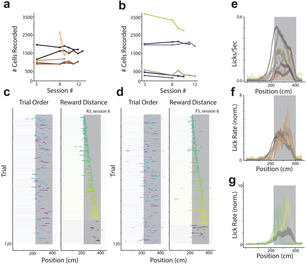
a, The number of cells identified per session is plotted for each rare morph animal individually. Each mouse shown as a different color. b, Same as (a) for all frequent morph animals. c, Single trial lick rate as a function of position is shown for an example rare morph session (R3, session 8; n = 120 trials). Left: Each row indicates the smoothed lick rate across positions for a single trial. The color of the row indicates the morph value (colormap in Fig. 1c). The grey shaded region indicates possible reward locations. Trials are shown in the order in which they occurred during the experiment. Right: Trials are sorted by the location of the reward cue. The color code also indicates increasing reward distance from the start of the track (green to yellow). Black trials are those in which the reward cue was omitted. d, Same as (c) for an example frequent morph session (F5, session 8; n = 120 trials). e, Across session mean lick rate (licks/sec) as a function of position (see [a-b] for number of sessions and color code) is plotted as a separated line for each mouse (R1-R6 & F1-F6; mean ± SEM). The color scheme for each mouse is the same as in the rest of the manuscript. Grey shaded region indicates possible reward location as in (c-d). f, The same data as (e) is normalized by the animal’s overall mean lick rate. g, Normalized mean lick rates were combined across rare and frequent morph animals. Trials were then binned by reward location (50 cm bins) and plotted as a function of position (across animal mean ± SEM). Color code is the same as (c-d).
Extended Data Fig. 2 ∣. Across Virtual Reality (VR) scene variance is best predicted by the horizontal component of the frequency of wall cues.
a, Schematic of how across scene covariance was determined. Screenshots of the virtual scene were taken at every 10 cm for the range of possible wall, tower, and background morph parameter settings. Translation invariant representations of these VR scenes were acquired by calculating the two-dimensional Fast Fourier Transform (FFT) of every screenshot on each color channel (RGB). Discarding phase information, we took the power spectrum for each channel and each screenshot. We flattened each of the FFT power spectrums into a column vector. Column vectors for every color channel and every position along the track were concatenated for a given morph parameter setting. This procedure gives one column vector for each morph parameter setting. We then horizontally stacked these column vectors for each morph parameter setting to give a matrix that we used to calculate a morph by morph covariance matrix. We then performed Principal Components Analysis (PCA) on this matrix. b, The eigenvalues of the morph by morph covariance matrix are plotted. c, The projection of each morph parameter setting onto the first principal component (PC1) from (a) plotted as a function of the wall morph value ( + wall jitter)(left vertical axis, blue points). The horizontal component of the frequency of the wall cues, fh, is also plotted (right vertical axis, red points). d, The projection of each morph parameter setting onto PC1 is plotted as a function of wall morph value (left vertical axis, blue points). The vertical component of the frequency of the wall cues, fv, is also shown (right vertical axis, red points). e, The projection of each morph parameter setting onto PC1 is plotted as a function of tower morph value (+ tower jitter)(left vertical axis, blue points). The normalized blue color channel pixel value of the towers is also plotted (right vertical axis, red points). The normalized green color channel pixel value of the tower is one minus the blue color channel. f, The projection onto PC1 is plotted as a function of background morph value (+ background jitter). The normalized background color pixel intensity is also plotted (right vertical axis, red points). g, The log of the mean squared error (log(MSE)) of a linear regression to predict the projection of morph parameter settings onto PC1 is plotted for models using different sets of predictors. The ‘all’ model uses fh, fv, background pixel value (b), tower blue pixel value (t), and the angle of the wall cues (angle) as predictors of the projection onto PC1. The failure of this model is likely due to the strong correlation among stimulus values. Every other model uses only a single aspect of the stimulus to predict the projection onto PC1. The horizontal component of wall frequency, fh, is the strongest predictor of the projection onto PC1. h, Ideal rare morph log posterior distribution as plotted Fig. 1f. i. Ideal frequent morph log posterior distribution as plotted Fig. 1f.
Extended Data Fig. 3 ∣. Remapping patterns for a simulated population designed to stochastically encode the posterior distribution reproduces our recorded remapping patterns.
a, Schematic for model of a ‘neural posterior’. Left: As the animal runs down the track, it tries to infer the identity of the environment it is occupying. The probability of the environment is given by the posterior distribution. Right: We assume that the activity of the neurons we are observing is governed by radial basis function tuning curves for distinct values of the inferred stimulus. b, Process for generating activity. Left: As the animal runs down the track, a process generates several random samples from the posterior distribution. Middle: Each of these samples is filtered through the deterministic neural tuning curves shown in (a). Right: Cellular activity rates are generated by a gamma process with parameters determined by the neural activation. Gamma processes were chosen, as calcium activity rate is a continuous variable. Mean and variance of gamma processes were chosen to be identical so they were more Poisson-like. c, Left: The ideal rare morph posterior distribution as plotted in Fig. 1f (top right) and elsewhere. Right: The activity of a simulated population that encodes samples from the rare morph posterior is shown for different fh values. Each row of the heat map is the activity of a single cell sorted by the fh values for which it has peak selectivity. Each column is the value of fh used to generate a draw from the posterior distribution. Color (white to purple) indicates the average activity of the cell across 1000 draws from the posterior distribution. Yellow points show the index in the population that has the highest average activity rate. Maroon points indicate the ideal rare morph MAP estimates as in left. Note the similarity between the ideal posterior distribution (left) and the activity of the population designed to encode it (right). d, Same as (c) for simulations using the ideal frequent morph posterior distribution. e, Example trial by trial similarity matrices for simulated populations encoding the rare morph posterior. f, Same as (e) for simulated populations encoding the frequent morph posterior. g, Average rare morph trial x trial similarity matrix (n = 1,000 simulations). h, Average frequent morph trial x trial similarity matrix (n = 1,000 simulations). i, Difference in mean trial x trial similarity matrices (rare [g] - frequent [h]). j, Same as (i) but similarity matrices are z-scored prior to averaging (diagonal elements excluded).
Extended Data Fig. 4 ∣. Analysis of place cells with place fields in both and environments, and analysis of posterior distribution entropy.
a, Fraction of cells classified as place cells in the trials (magenta), trials (cyan), and both and trials (intersection of the sets of cells; navy). The number of cells expected to be classified as place cells in both environments if cells were chosen randomly with replacement is also shown (red). b, For cells that were classified as place cells in both and trials (n = 2,219 cells) in rare morph animals, we plotted the location of peak activity for trials against the location of peak activity for trials. Marginal histograms are shown for occupancy of position bins in the trials (bottom) and trials (right). Shaded regions indicate possible reward locations. c, Same as (b) for all frequent morph animals (n = 594 cells). d, Same as Fig. 2b (rare morph condition) but only cells that had place fields in both and trials are plotted (n = 2,219 cells). e, Same as Fig. 2d (frequent morph condition) but only cells that had place fields in both and trials are plotted (n = 594 cells). f, Example posterior distributions (rare morph-maroon, frequent morph-blue) for different values of (that is columns of Fig. 1f). g, Entropy of the posterior distribution as a function of (rare morph-maroon, frequent morph-blue).
Extended Data Fig. 5 ∣. Unsupervised confirmation of discrete vs continuous remapping.
a, Schematic of nonlinear dimensionality reduction. Morph-binned spatial activity rate maps were generated for cells with significantly different activity rate maps between and . Morph by position maps were flattened and then stacked to form a cells x (position bins*morph bins) matrix. We performed UMAP dimensionality reduction on this matrix. This produces an embedding space for plotting individual cells. In this space, cells with similar activity rate maps are close together, and cells with dissimilar activity rates are further apart, b, Three-dimensional embedding given by UMAP colored by different experimentally relevant variables. Top Left: Cells/points are colored by the morph value for which their activity is the highest (color bar right). Top Right: Cells/points are colored by their position of peak activity (color bar right). Bottom Left: Cells/points are colored by whether they came from the rare morph condition (orange) or frequent morph condition (blue). Bottom Right: Density based clustering was performed to separate the two main manifolds. K-means clustering was performed on each of the manifolds (10 clusters per manifold, 20 total clusters [numbered on plot], colors correspond to different clusters). c, Decoding performance (logistic regression) for classifying cells as coming from the rare morph or frequent morph condition for each cluster from the S = 0 manifold (magenta, Top) or from the S = 1manifold (cyan, Bottom). Classification accuracy is plotted as a function of the spatial preference of that cluster. Grey shaded region indicates the range of chance performance by permutation test (n = 1,000 permutations). Red shaded regions highlight reward locations d, Average remapping patterns for rare and frequent morph cells within an example cluster (b, lower right). For each cluster, we give the rare vs. frequent classification accuracy. For each example cluster, we plot the cell averaged morph-binned activity rate map for rare morph (first column, top) and frequent morph (second column, top) cells as well as the associated cosine similarity matrix (bottom). Third column shows the difference between the first and second column (Rare-Freq.). Black arrows indicate S = 0.25–.5 region where magnitude of difference is expected to be the largest.
Extended Data Fig. 6 ∣. Nonnegative matrix factorization on population of single cell trial by trial similarity matrices confirms discrete (rare morph) versus continuous remapping (frequent morph).
a, Schematic for how Nonnegative Matrix Factorization (NMF) was performed. For each cell within an imaging session, we flattened the upper triangle of its trial by trial similarity matrix (as seen in Fig. 1g,i) to form a vector. These vectors were then stacked to form a Neurons × (Trials * (Trials – 1)/2) matrix, X. NMF was then performed on this matrix yielding a factors matrix, HT, and a loadings matrix, W. The rows of HT can be reshaped into ‘prototypical similarity matrices’. b, NMF factors for rank three models for example rare morph sessions from each rare morph mouse. Color coding indicates maximum (yellow) and minimum (blue) values. c, Same as (b) for example sessions from each frequent morph mouse.
Extended Data Fig. 7 ∣. Population similarity analyses from every rare morph session and mouse.
The animal from which data is derived is shown in large bold text above (for example R1). For each animal, each row of plots indicates data from a single session sorted by increasing session number. Session 3 data is included for all animals except R6. Left: Trial by trial population similarity matrices are shown, sorted by morph value (lower plot), as in Fig. 3a. Right: Q estimates (estimates of ) for given session. ΔDKL value is given for each session.
Extended Data Fig. 8 ∣. Population similarity analyses from every frequent morph session and mouse.
The animal from which data is derived is shown in large bold text above (for example F1). For each animal, each row of plots indicates data from a single session sorted by increasing session number. Session 3 data is included for all animals. Left: Trial by trial population similarity matrices are shown, sorted by morph value (lower plot), as in Fig. 3a. Right: Q estimates (estimates of ) for given session. ΔDKL value is given for each session.
Extended Data Fig. 9 ∣. Session 3 remapping patterns are consistent with later session remapping in the majority of animals, and results are poorly fit by null posterior distributions.
a, Left Column: Trial by trial similarity matrices for session 3 from two rare morph mice (R3-1,973, 90 trials; R4-922 cells, 60 trials). Trials sorted by increasing morph value. Right column: Q estimates for example sessions. b, Same as (a) for example frequent morph sessions (F6, 3,657 neurons, 100 trials; F3, 295 cells, 120 trials). c, ΔDKL for each rare morph mouse plotted as a function of session number. Session 3 data unavailable for R6. d, Same as (c) for frequent morph animals. e, Q estimate for accumulated session 3 data across rare morph mice, f, Same as (e) for frequent morph mice, g-h, Reconstructed prior distributions for rare (g) and frequent (h) morph mice using session 3 data alone. Average rare (maroon) and frequent (blue) morph prior are shown. i, Relative distance of reconstructed priors to ideal priors, ΔDKL, for each mouse (rare mice-left; frequent mice-right). j, Top: Prior distributions for additional models tested for comparison with Q estimates. Bottom: Associated posterior distributions for each prior. We additionally compared Q estimates to a uniform posterior (, where c is a constant). k, Left: Kullback-Leibler divergence (DKL) between each posterior in (j) and the Q estimate. Points are colored by mouse ID. Thick maroon line indicates the across session average. (***) indicate significant differences in DKL with the rare morph DKL values (Wilcoxon signed-rank test, n = 24 sessions; frequent, p = 2.3 × 10⁻⁴; uniform, p = 4.7 × 10⁻⁴; Gaussian, p = 1.8 × 10⁻⁵; multimodal, p = 1.8 × 10⁻⁵; uniform posterior, p = 1.82 × 10⁻⁵). Right: DKL between reconstructed prior and different priors shown in (j). I, Same as (k) for frequent morph sessions. Left: Thick blue line indicates across session average. Wilcoxon signed rank tests compare DKL for the frequent morph condition to DKL for all other posteriors in (j) (Wilcoxon signed-rank test, n = 21 sessions; rare, p = 6.0 × 10⁻⁵; uniform, p = 0.019; Gaussian, p = 6.0 × 10⁻⁵; multimodal, p = 6.0 × 10⁻⁵; uniform posterior, p = 6.0 × 10⁻⁵).
Extended Data Fig. 10 ∣. Requiring frequent morph animals to behaviorally categorize morph values does not change neural context discrimination.
a, Stimulus design, as in Fig. 1b, for frequent morph trained animals that had to behaviorally categorize morph values (frequent morph with decision, n = 4 animals, FD1-FD4). A side view of a subset of VR tracks with different morph values (S) are shown. Vertical location indicates approximate morph value for the track shown (color bar to the right of tracks). For trials where S ≤ 0.5, animals had to lick within a 65 cm region surrounding the third tower (polka dot tower, magenta highlighted region). For trials where S > 0.5, animals had to lick within a 65 cm region surrounding the fourth tower (hatched pattern tower, cyan highlighted region). For one animal (FD1), we added punishments for licking in the incorrect reward zone after session 3. If the animal licked in the incorrect reward zone, it was instantly teleported to a dark hallway for 10 seconds before being able to begin the next trial. b, Left: Lick rate as a function of position for each trial as in Extended Data Fig. 1c,d for an example session (FD1, session 13, n = 120 trials). Red dots indicate error. Color indicates morph value of the trial. Shaded regions indicate reward zones as in (a). Right: Trials are sorted by increasing morph value c, For mice that did not receive timeouts for incorrect licks (n = 3, FD2-4), we plot the across mouse average normalized lick rate (normalization as in Extended Data Fig. 1) as a function of position (across mouse mean ± SEM) for binned morph values (, 0.25, 0.5, 0.75, 1). d. Far Left: Trial by trial cosine similarity matrix sorted by increasing morph value for an example session from the mouse that experienced timeouts (FD1, session 13; 120 trials, 1451 cells). Middle Left: Projection of single trials onto the principal two eigenvectors of the similarity matrix. Color indicates morph value. Middle Right: Similarity Fraction, SF, as a function of position as in Fig. 3f. Color indicates morph value. Far Right: Q estimates. e, Same as (d) for an example session from an animal that did not receive timeouts for incorrect licks (FD4, session 12; 100 trials, 924 cells). f, Q estimate using pooled data across all FD mice. g, Background heatmap is the ideal frequent morph posterior distribution. Blue scatterplot points are the MAP estimate from this ideal posterior. Remaining overlaid scatterplot is the linearly transformed SF(fh) values for every trial and every mouse (N = 2,460 trials). Colors indicate mouse ID. h, Reconstructed prior distributions for each FD mouse. Maroon thick plot indicates ideal rare morph prior, blue thick plot indicates ideal frequent morph prior, thinner lines indicate individual mouse reconstructions. Colors indicate mouse ID as in (g).
Supplementary Material
Acknowledgements
This work was supported by funding from the New York Stem Cell Foundation, the Office of Naval Research (N00141812690), the Simons Foundation (542987SPI), the Vallee Foundation and the James S. McDonnell Foundation to L.M.G., and a National Science Foundation Graduate Research Fellowship awarded to M.H.P. We thank A. Diaz for histology and behavioral training assistance. We thank K. Hardcastle, A. H. Williams and S. Ganguli for helpful discussions regarding data analyses and modeling, and A. Drinnenberg and K. Kaganovsky for providing feedback on the manuscript.
Footnotes
Online content
Any methods, additional references, Nature Research reporting summaries, source data, extended data, supplementary information, acknowledgements, peer review information; details of author contributions and competing interests; and statements of data and code availability are available at https://doi.org/10.1038/s41593-021-00816-6.
Reporting Summary. Further information on research design is available in the Nature Research Reporting Summary linked to this article.
Code availability
The computer code used for analysis and simulations, as well as creating and controlling VR environments in Unity, is available at https://github.com/GiocomoLab/PlittGiocomo_2021.
Competing interests
The authors declare no competing interests.
Extended data is available for this paper at https://doi.org/10.1038/s41593-021-00816-6.
Supplementary information The online version contains supplementary material available at https://doi.org/10.1038/s41593-021-00816-6.
Data availability
The datasets generated during the current study are available in the DANDI repository (https://dandiarchive.org/dandiset/000054/draft).
References
- 1.O’Keefe J & Dostrovsky J The hippocampus as a spatial map. Preliminary evidence from unit activity in the freely-moving rat. Brain Res 34, 171–175 (1971). [DOI] [PubMed] [Google Scholar]
- 2.Bostock E, Muller RU & Kubie JL Experience-dependent modifications of hippocampal place cell firing. Hippocampus 1, 193–205 (1991). [DOI] [PubMed] [Google Scholar]
- 3.Colgin LL et al. Attractor-map versus autoassociation based attractor dynamics in the hippocampal network. J. Neurophysiol 104, 35–50 (2010). [DOI] [PMC free article] [PubMed] [Google Scholar]
- 4.Knierim JJ, Kudrimoti HS & McNaughton BL Interactions between idiothetic cues and external landmarks in the control of place cells and head direction cells. J. Neurophysiol 80, 425–446 (1998). [DOI] [PubMed] [Google Scholar]
- 5.Leutgeb JK et al. Progressive transformation of hippocampal neuronal representations in ‘morphed’ environments. Neuron 48, 345–358 (2005). [DOI] [PubMed] [Google Scholar]
- 6.Leutgeb S, Leutgeb JK, Treves A, Moser MB & Moser EI Distinct ensemble codes in hippocampal areas CA3 and CA1. Science 305, 1295–1298 (2004). [DOI] [PubMed] [Google Scholar]
- 7.Lever C, Wills T, Cacucci F, Burgess N & O’Keefe J Long-term plasticity in hippocampal place-cell representation of environmental geometry. Nature 416, 236–238 (2002). [DOI] [PubMed] [Google Scholar]
- 8.Muller RU & Kubie JL The effects of changes in the environment on the spatial firing of hippocampal complex-spike cells. J. Neurosci 7, 1851–1868 (1987). [DOI] [PMC free article] [PubMed] [Google Scholar]
- 9.O’Keefe J & Conway DH Hippocampal place units in the freely moving rat: why they fire where they fire. Exp. Brain Res 31, 573–590 (1978). [DOI] [PubMed] [Google Scholar]
- 10.Wills TJ, Lever C, Cacucci F, Burgess N & O’Keefe J Attractor dynamics in the hippocampal representation of the local environment. Science 308, 873–876 (2005). [DOI] [PMC free article] [PubMed] [Google Scholar]
- 11.Colgin LL, Moser EI & Moser MB Understanding memory through hippocampal remapping. Trends Neurosci 31, 469–477 (2008). [DOI] [PubMed] [Google Scholar]
- 12.Lee I, Yoganarasimha D, Rao G & Knierim JJ Comparison of population coherence of place cells in hippocampal subfields CA1 and CA3. Nature 430, 456–459 (2004). [DOI] [PubMed] [Google Scholar]
- 13.Sanders H, Wilson MA & Gershman SJ Hippocampal remapping as hidden state inference. eLife 9, e51140 (2020). [DOI] [PMC free article] [PubMed] [Google Scholar]
- 14.McInnes L, Healy J & Melville J UMAP: uniform manifold approximation and projection for dimension reduction. Preprint at arXiv https://arxiv.org/abs/1802.03426 (2018). [Google Scholar]
- 15.Rolls ET in The Neural and Molecular Bases of Learning (eds Changeux J-P & Konishi M) 503–540 (Wiley, 1987). [Google Scholar]
- 16.McNaughton BL & Morris RGM Hippocampal synaptic enhancement and information storage within a distributed memory system. Trends Neurosci 10, 408–415 (1987). [Google Scholar]
- 17.Fiser J, Berkes P, O’rban G & Lengyel M Statistically optimal perception and learning: from behavior to neural representations. Trends Cogn. Sci 14, 119–130 (2010). [DOI] [PMC free article] [PubMed] [Google Scholar]
- 18.Pouget A, Beck JM, Ma WJ & Lathan PE Probabilistic brains: knowns and unknowns. Nat. Neurosci 16, 1170–1178 (2013). [DOI] [PMC free article] [PubMed] [Google Scholar]
- 19.Nessler B, Pfieffer M, Buesing L & Maass W Bayesian computation emerges in generic cortical microcircuits through spike-timing-dependent plasticity. PLoS Comput. Biol 9, e1003037 (2013). [DOI] [PMC free article] [PubMed] [Google Scholar]
- 20.Keinath AT, Nieto-Posadas A, Robinson JC & Brandon MP DG–CA3 circuitry mediates hippocampal representations of latent information. Nat. Commun 11, 3026 (2020). [DOI] [PMC free article] [PubMed] [Google Scholar]
- 21.Chen S et al. A hypothalamic novelty signal modulates hippocampal memory. Nature 586, 270–274 (2020). [DOI] [PubMed] [Google Scholar]
- 22.Keinath AT, Mosser CA & Brandon MP Extended experience reveals distinct representational dynamics governing the CA1 spatial code. Preprint at bioRxiv 10.1101/2021.01.12.426395 (2021). [DOI] [Google Scholar]
- 23.Sheffield MEJ & Dombeck DA Increased prevalence of calcium transients across the dendritic arbor during place field formation. Neuron 96, 490–504 (2017). [DOI] [PMC free article] [PubMed] [Google Scholar]
- 24.Aronov D & Tank DW Engagement of neural circuits underlying 2D spatial navigation in a rodent virtual reality system. Neuron 84, 442–456 (2014). [DOI] [PMC free article] [PubMed] [Google Scholar]
- 25.Cohen JD, Bolstad M & Lee AK Experience-dependent shaping of hippocampal CA1 intracellular activity in novel and familiar environments. eLife 6, e23040 (2017). [DOI] [PMC free article] [PubMed] [Google Scholar]
- 26.Danielson NB et al. Sublayer-specific coding dynamics during spatial navigation and learning in hippocampal area CA1. Neuron 91, 652–665 (2016). [DOI] [PMC free article] [PubMed] [Google Scholar]
- 27.Hainmueller T & Bartos M Parallel emergence of stable and dynamic memory engrams in the hippocampus. Nature 558, 292–296 (2018). [DOI] [PMC free article] [PubMed] [Google Scholar]
- 28.Acharya L, Aghajan ZM, Vuong C, Moore JJ & Mehta MR Causal influence of visual cues on hippocampal directional selectivity. Cell 164, 197–207 (2016). [DOI] [PubMed] [Google Scholar]
- 29.Aghajan ZM et al. Impaired spatial selectivity and intact phase precession in two-dimensional virtual reality. Nat. Neurosci 18, 121–128 (2015). [DOI] [PubMed] [Google Scholar]
- 30.Marr D Simple memory: a theory for archicortex. Philos. Trans. R. Soc. Lond. B Biol. Sci 262, 23–81 (1971). [DOI] [PubMed] [Google Scholar]
- 31.Hopfield JJ Neural networks and physical systems with emergent selective computational abilities. Proc. Natl Acad. Sci. USA 79, 2554–2559 (1982). [DOI] [PMC free article] [PubMed] [Google Scholar]
- 32.Lever C, Burgess N, Cacucci F, Hartley T & O’Keefe J What can the hippocampal representation of environmental geometry tell us about Hebbian learning? Biol. Cybern 87, 356–372 (2002). [DOI] [PubMed] [Google Scholar]
- 33.Stachenfeld KL, Botvinick MM & Gershman SJ The hippocampus as a predictive map. Nat. Neurosci 20, 1643–1653 (2017). [DOI] [PubMed] [Google Scholar]
- 34.Samsonovich A & McNaughton BL Path integration and cognitive mapping in a continuous attractor neural network model. J. Neurosci 17, 5900–5920 (1997). [DOI] [PMC free article] [PubMed] [Google Scholar]
- 35.Hedrick KR & Zhang K Megamap: flexible representation of a large space embedded with nonspatial information by a hippocampal attractor network. J. Neurophysiol 116, 868–891 (2016). [DOI] [PMC free article] [PubMed] [Google Scholar]
- 36.Wilson RC & Finkel LH A neural implementation of the Kalman Filter. Adv. Neural Inf. Process. Syst 22, 2728–2736 (2009). [Google Scholar]
- 37.Deneve S, Duhamel JR & Pouget A Optimal sensorimotor integration in recurrent cortical networks: a neural implementation of Kalman filters. J. Neurosci 27, 5744–5756 (2007). [DOI] [PMC free article] [PubMed] [Google Scholar]
- 38.Aronov D, Nevers R & Tank DW Mapping of a non-spatial dimension by the hippocampal-entorhinal circuit. Nature 543, 719–722 (2017). [DOI] [PMC free article] [PubMed] [Google Scholar]
- 39.Constantinescu AO, O’Reilly JX & Behrens TE Organizing conceptual knowledge in humans with a gridlike code. Science 352, 1464–1468 (2016). [DOI] [PMC free article] [PubMed] [Google Scholar]
- 40.Tsien JZ et al. Subregion- and cell type-restricted gene knockout in mouse brain. Cell 87, 1317–1326 (1996). [DOI] [PubMed] [Google Scholar]
- 41.Dana H et al. High-performance calcium sensors for imaging activity in neuronal populations and microcompartments. Nat Methods 16, 649–657 (2019). [DOI] [PubMed] [Google Scholar]
- 42.Lovett-Barron M et al. Dendritic inhibition in the hippocampus supports fear learning. Science 343, 857–863 (2014). [DOI] [PMC free article] [PubMed] [Google Scholar]
- 43.Dombeck DA, Harvey CD, Tian L, Looger LL & Tank DW Functional imaging of hippocampal place cells at cellular resolution during virtual navigation. Nat Neurosci 13, 1433–1440 (2010). [DOI] [PMC free article] [PubMed] [Google Scholar]
- 44.Skaggs WE, McNaughton BL, Gothard KJ & Markus EJ An information-theoretic approach to deciphering the hippocampal code. Adv. Neural Inf. Process. Syst 5, 1030–1037 (1993). [Google Scholar]
Associated Data
This section collects any data citations, data availability statements, or supplementary materials included in this article.
Supplementary Materials
Data Availability Statement
The datasets generated during the current study are available in the DANDI repository (https://dandiarchive.org/dandiset/000054/draft).


