Hawkes Processes Framework With a Gamma Density As Excitation Function: Application to Natural Disasters for Insurance

Abstract

Hawkes processes are temporal self-exciting point processes. They are well established in earthquake modelling or finance and their application is spreading to diverse areas. Most models from the literature have two major drawbacks regarding their potential application to insurance. First, they use an exponentially-decaying form of excitation, which does not allow a delay between the occurrence of an event and its excitation effect on the process and does not fit well on insurance data consequently. Second, theoretical results developed from these models are valid only when time of observation tends to infinity, whereas the time horizon for an insurance use case is of several months or years. In this paper, we define a complete framework of Hawkes processes with a Gamma density excitation function (i.e. estimation, simulation, goodness-of-fit) instead of an exponential-decaying function and we demonstrate some mathematical properties (i.e. expectation, variance) about the transient regime of the process. We illustrate our results with real insurance data about natural disasters in Luxembourg.

Summary

Hawkes Processes

Hawkes processes form a specific category of point processes. Their main characteristic is that each event “self-excites” the process, which means that an occurrence increases the probability to have another arrival in a short time period. They were first introduced by Hawkes (1971) and are now commonly used for several applications: earthquake modelling Bacry and Muzy (2014), criminology Mohler (2011), finance Bacry et al. (2015), etc.

Hawkes Processes for Insurance

Since recently, insurance companies are developing an interest for Hawkes processes. They are used for calculating Solvency Capital Requirements and modelling different indicators of risks, such as ruin (improvement of Cramer-Lundberg model, see Cheng and Seol (2020)) or cyber-attacks (see Bessy-Roland et al. (2020)). Hawkes processes model claims arrival, considered to follow a Poisson process in classic approaches.

Article Purpose

Up to now, models using Hawkes processes in the literature mainly use an exponential excitation function, whose theory was developed in Hawkes’ original papers Hawkes (1971). For this excitation function, the self-exciting effect of each occurrence is maximal shortly after the event. However, for most insurance use cases, we need to take into account a delay between the event and its exciting effect on the process. The main originality of this paper is to propose the Gamma density as an excitation function suited to this context and to test on real data that this approach is a better choice in insurance situations. We introduce and discuss some practical situations on which the Gamma density fits better than exponential decay. The Gamma density excitation function allows us to deal with this delay and could be seen as a generalization of the exponential excitation function, since both are equivalent for a particular set of parameters.

At our best knowledge in the literature, there only exists limit results on first and second order statistics about this category of Hawkes processes. In Bacry and Muzy (2014), the authors state the Wiener-Hopf equations followed by the kernel matrix functions for all t. They only compute the expectation of a Hawkes process in a stationary state. In Bacry et al. (2012), the focus is on the asymptotic behaviour of multivariate Hawkes processes for a large time, by stating a law of large numbers and a functional central limit theorem. In Bordenave and Torrisi, Large deviations of Poisson cluster processes. Bordenave and Torrisi (2007) (Gao and Wang (2020) resp.), the authors prove a so-called large (moderate resp.) deviations principle on Hawkes processes. Such limit results established on the stationary regime are not suitable to deal with practical cases in the insurance context, where the time horizon is of several months. In this paper, we develop a framework for Hawkes processes with Gamma density excitation function regarding estimation and simulation. A new result in this context is the calculus of the mean and the variance of the process in the transient regime. To illustrate our work, we develop the use case of natural disasters in Luxembourg.

Main Contributions

The major contributions of this paper are to:

1. Define Hawkes processes and the elements needed for a complete use case study (estimation, goodness-of-fit, simulation, etc.);

2. Study mathematical expressions and properties of Hawkes processes (i.e. expectation, variance and central limit theorem) with a Gamma density as excitation function;

3. Model an insurance use case with real data by this specific form of Hawkes processes as an illustration of the mathematical tools.

Plan

The remainder of this paper is organized as follows. The second section defines a Hawkes process and introduces all useful notations. The third section contains the development of our results on mathematical properties of Hawkes processes. We also study a use case applied to insurance in the fourth section (natural disasters in Luxembourg).

Hawkes Processes Definition

In this section, we define the notion of Hawkes process, and we introduce useful notations for mathematical properties and algorithms (simulation, estimation).

Point Process

Hawkes processes are a particular class of point processes. We first propose a definition of a point process, inspired by Daley and Vere-Jones (2003).

Definition 1

(Point Process). A point process $\mathbf{T}$ is an increasing sequence of random variables $\mathbf{T}=\{T_1,T_2,...\}$ called occurrences which takes values in $[0,+\infty [$, such that $\mathbb{P}(0\le T_1\le T_2\le ...)=1$.

Definition 2

(History of Occurrences). We define ($\mathcal{H}(t),t\ge 0$) the filtration and the history of the occurrences until time t.

Another useful representation of a sequence of occurrences is the counting notation.

Definition 3

(Counting Process). We say that N is a counting process if it is an almost surely finite stochastic process and a right-continuous step function with +1 increments after each step, taking values in $\mathbb{N}$, and $N(0)=0$.

The two notions of point process and counting process are interchangeable. Indeed, a counting process could be seen as the cumulative count of a point process. The link between $\mathbf{T}$ and N is:

$$\begin{array}{c}\hfill \forall t\in {\mathbb{R}}_{+},N(t)=\#\{T_i\in \mathbf{T}|T_i\le t\},i\ge 1,\end{array}$$

where $\#$ denotes the cardinality of a set and $T_i$ is the time of the $i^{\mathit{th}}$ occurrence in the time interval [0, T], where Tis the final time of observation.

Intensity Function

The most frequently used characterization of a Hawkes process is by means of the conditional intensity function, $\lambda (t|\mathcal{H}(t))$. It is defined below.

Definition 4

(Conditional Intensity Function: Expected Rate of Occurrences Conditioned on $\mathcal{H}(t)$). Let us consider a counting process $N(·)$. If $\lambda (t|\mathcal{H}(t))$ exists such that:

$$\begin{array}{c}\hfill \lambda (t|H(t))=\underset{h\to 0^{+}}{lim}\frac{\mathbb{E}[N(t+h)-N(t)|\mathcal{H}(t)]}{h},\end{array}$$ 1

then $\lambda (t|\mathcal{H}(t))$ is the conditional intensity function of $N(·)$. We denote $\lambda (t|\mathcal{H}(t))$ by ${\lambda }^{\ast }(t)$ for the remainder of the paper.

The following proposition is inspired from Proposition 2.2 of Rasmussen (2018) and states that the conditional intensity function uniquely defines the point process. Thus in the following we use this characterization.

Proposition 1

Let us consider a conditional intensity function ${\lambda }^{\ast }(·)$, defined for any time period [u, t], $0\le u\le t$, such that:

• ${\lambda }^{\ast }(·)$ non-negative and integrable on [u, t],

• $\underset{t\to +\infty }{lim}$ ${\int }_u^t{\lambda }^{\ast }(s)ds=+\infty$.

Then there exists an unique point process with ${\lambda }^{\ast }(t)$ conditional intensity function.

Hawkes Process Definition

We introduce now the definition of Hawkes processes.

Definition 5

(Hawkes Process). Let us consider $\lambda >0$, the background intensity, and $\mu :[0,+\infty [\to [0,+\infty [$, the excitation function. We denote $\{t_1,..,t_{N(t)}\}$ the sequence of past occurrences until time t. A point process is a Hawkes process if its conditional intensity function is of the form:

$$\begin{array}{c}\hfill {\lambda }^{\ast }(t)=\lambda +{\int }_0^t\mu (t-u)dN(u)=\lambda +\sum _{k=1}^{N(t)}\mu (t-t_k),\end{array}$$ 2

where $N(·)$ is defined in Definition 3.

Hawkes processes are point processes who have a so-called “self-exciting” property. It means that each occurrence increases the intensity, according to the excitation function. A higher intensity leads to more occurrences, leading to a higher frequency, etc. A Hawkes process with a null excitation function is a homogeneous Poisson process of rate $\lambda$.

Definition 6

($\mathrm{\Gamma }$-Hawkes Processes). We define the $\mathrm{\Gamma }$-Hawkes processes, a Hawkes process whose excitation function is of form:

$$\begin{array}{c}\hfill \mu (t)=\alpha \frac{t^{k_1-1}exp(-\frac{t}{k_2})}{k_2^{k_1}\mathrm{\Gamma }(k_1)},t\ge 0,\alpha \in {\mathbb{R}}_{+}^{\ast },k_1,k_2\in {\mathbb{R}}_{+}^{\ast },\end{array}$$ 3

where $\mathrm{\Gamma }(·)$ is the Gamma function. $k_1$ is the scale parameter and $k_2$ is the shape parameter.

Remark 1

For $k_1=1$, we obtain the exponential excitation function:

$$\begin{array}{c}\hfill \mu (t)=\alpha \frac{exp(-\frac{t}{k_2})}{k_2},t\ge 0,\alpha \in {\mathbb{R}}_{+}^{\ast },k_2\in {\mathbb{R}}_{+}^{\ast },\end{array}$$ 4

used for instance originally by Hawkes (1971). In this situation:

$$\begin{array}{c}\hfill {\lambda }^{\ast }(t)=\lambda +\sum _{k=1}^{N(t)}\alpha \frac{exp(-\frac{t-t_k}{k_2})}{k_2}.\end{array}$$ 5

For $k_1>1$, this excitation function allows to avoid a discontinuity in the intensity function when an event occurs, and introduce a delay between an event and its impact on the process. Indeed, in that case, $\mu (0)=0$. This property is very helpful when considering events for which an occurrence and the resulting self-excitation are delayed.

Mathematical Properties

In this section, we are going to explicit some mathematical properties of the $\mathrm{\Gamma }$-Hawkes processes (defined by Eq. (3)): we calculate the expectation and the variance for any time $t\ge 0$ and we state a central limit theorem.

Assumption 1

For the whole Section 3, we consider a $\mathrm{\Gamma }$-Hawkes process of conditional intensity function:

$$\begin{array}{c}\hfill {\lambda }^{\ast }(t)=\lambda +{\int }_0^t\mu (t-u)dN(u)=\lambda +\alpha \sum _{k=1}^{N(t)}\frac{{(t-t_k)}^{k_1-1}exp(\frac{-(t-t_k)}{k_2})}{k_2^{k_1}\mathrm{\Gamma }(k_1)},\end{array}$$ 6

where $\alpha \in {\mathbb{R}}_{+}^{\ast },k_1,k_2\in {\mathbb{R}}_{+}^{\ast }$, $N(t)\ge 0$ (number of events occurred between 0 and t), $t_k$, $k\in \{1,...,N(t)\}$ for which we are going to explicit results for $k_1=1$ and $k_1=2$.

This study aims to understand the behaviour of the Hawkes processes in function of parameters introduced previously.

Behaviour in Function of Values of $\alpha$

In this section, we are going to see that the Hawkes process dynamics depend on values of $\alpha$ (defined in Assumption 1). To do so, let us focus on $g(t)=\mathbb{E}[{\lambda }^{\ast }(t)]$, which will be used to calculate the expectation of the Hawkes process later.

We could show that g follows a renewal equation:

$$\begin{array}{c}\hfill g(t)=\lambda +{\int }_0^t\mu (t-u)g(u)du.\end{array}$$ 7

According to Asmussen (2003), the behaviour of g(t), when t goes to infinity, depends on the value of:

$$\begin{array}{c}\hfill {\int }_0^{+\infty }\mu (u)du={\int }_0^{+\infty }\alpha \frac{{\beta }^{k_1}{u}^{k_1-1}exp(-\beta u)}{\mathrm{\Gamma }(k_1)}du=\alpha .\end{array}$$ 8

We distinguish, in the classic literature about point processes:

• The defective case: $\alpha <1$;

• The proper case: $\alpha =1$;

• The excessive case: $\alpha >1$.

The Hawkes process intensity goes to infinity in the excessive case, leading to an explosion of the counting process. This situation does not suit to any real event we would like to model. The proper case is not studied here, because it does not correspond to a real case. We concentrate our attention in the defective case. In this case, g admits a finite limit in $+\infty$, which will be calculated later.

Assumption 2

For the rest of the Section 3, we consider a Hawkes process of conditional intensity function described in Assumption 1, with $0<\alpha <1$ (defective case).

Expectation: $\mathbb{E}(N(t))$

The first indicator that seems relevant for our study was the evaluation of the average number of events through time. We propose a calculation method which could be applied for any value of $k_1\in {\mathbb{N}}^{\ast }$. We will develop the calculations for two values of the shape parameter: $k_1=1$ (exponential excitation function), $k_1=2$ and $k_1=3$. Since a Hawkes process is the sum of a background part of intensity $\lambda$ and an self-exciting part, we expect that the expectation is higher than for a Poisson process of parameter $\lambda$, which is $\lambda t$ for all time $t>0$.

Proposition 2

The expectation of the $\mathrm{\Gamma }$-Hawkes process (i.e. conditional intensity function given by Eq. (6)) is:

1. For $k_1=1$ (i.e. $\mu (t)=\alpha \frac{exp(-\frac{t}{k_2})}{k_2}$, exponential decay):

   $$\begin{array}{c}\hfill \mathbb{E}(N(t))=\frac{\lambda }{1-\alpha }t-\frac{\alpha \lambda k_2}{{(1-\alpha )}^2}[1-exp(-\frac{1-\alpha }{k_2}t)].\end{array}$$ 9
2. For $k_1=2$ (i.e. $\mu (t)=\alpha \frac{texp(-\frac{t}{k_2})}{k_2^2}$):

   $$\begin{array}{c}\hfill \mathbb{E}(N(t))=\frac{\lambda }{1-\alpha }t+\frac{\lambda \sqrt{\alpha }{k}_2}{2{(1+\sqrt{\alpha })}^2}[1-exp(-\frac{1+\sqrt{\alpha }}{k_2}t)]\\ \hfill -\frac{\lambda \sqrt{\alpha }{k}_2}{2{(1-\sqrt{\alpha })}^2}[1-exp(-\frac{1-\sqrt{\alpha }}{k_2}t)].\end{array}$$ 10
3. For $k_1=3$ (i.e. $\mu (t)=\alpha \frac{t^{2}exp(-\frac{t}{k_2})}{k_2^3\mathrm{\Gamma }(3)}$):

   $$\begin{array}{c}\hfill \mathbb{E}(N(t))=\frac{\lambda }{1-\alpha }t+\frac{\lambda \alpha B}{k_2^3}exp(-r_{1}t)+\frac{\lambda \alpha C}{k_2^3}cos(\omega t)exp(-at)+\frac{\lambda \alpha (D-Ca)}{k_2^3\omega }sin(\omega t)exp(-at),\end{array}$$ 11

   where

   $$\begin{array}{cc}\hfill B& =\frac{1}{r_1(r_1{a}_1-r_1^2-a_2)},C=\frac{r_1-a_1}{a_2(r_1{a}_1-r_1^2-a_2)},D=\frac{r_1{a}_1-a_1^2+a_2}{a_2(r_1{a}_1-r_1^2-a_2)},\hfill \\ \hfill r_1& =\frac{1-{\alpha }^{1/3}}{k_2},a_1=\frac{(2+{\alpha }^{1/3})}{k_2},a_2=\frac{(1-\alpha )}{(1-{\alpha }^{1/3})k_2^2},a=\frac{(2+{\alpha }^{1/3})}{2k_2},\omega =\frac{\sqrt{3}{\alpha }^{1/3}}{2k_2}.\hfill \end{array}$$

See Appendix 1 for the proof, which is based on Laplace transform of $g(t)=\mathbb{E}({\lambda }^{\ast }(t))$ and could be applied for any value of $k_1$. We could notice that despite the formula complexity increases with $k_1$, we could observe several common trends. We first notice that for $\alpha \to 0$ (null excitation function), we obtain $\mathbb{E}(N(t))\underset{\alpha \to 0}{⟶}\lambda t$. This result is natural since we already mentioned that a Hawkes process with a null excitation function is equivalent to a Poisson process of parameter $\lambda$. For all values of the shape parameter, the expectation reveals three regimes for the $\mathrm{\Gamma }$-Hawkes process. As an example, we represent the expectation for $k_1=1,k_2=9,\alpha =0.9,\lambda =0.3$, which follows Eq. (9), in Fig. 1. It contains four plots:

• Top-left: expectation from Eq. (9) in blue and the so-called stationary regime $t\to \frac{\lambda }{1-\alpha }t$ in red, from t = 0 to 3000;

• Bottom-left: the relative difference between the expectation and the stationary regime on this time period;

• Top-right: focus on the expectation from t = 0 to 500;

• Bottom-right: plot of the exponential term from Eq. (9), $t\to exp(-\frac{1-\alpha }{k_2}t)$.

Fig. 1.

Number of claims per day processed by Foyer Assurances and labelled as natural disasters since 2015

We distinguish three regimes in this example:

• The transient regime (from t = 0 to 500 approximately): it is the time period necessary for the exponential term in Eq. (9) to become null;

• The intermediary regime (from t = 500 to 2000 approximately): the exponential term is null but the constant term could not be neglected before the stationary regime. On this period, the relative difference between the expectation and the stationary regime is above 5$\%$;

• The stationary regime: for any value of the parameter scale, and for any Hawkes process (not only for $\mathrm{\Gamma }$-Hawkes processes), $\mathbb{E}(N(t))\underset{t\to +\infty }{\sim }\frac{\lambda }{1-\alpha }t$ (see Gao (2018)). The constant term in Eq. (9) becomes negligible before the linear term. After the first two regimes, the average number of occurrences of the Hawkes process is the same as for a Poisson process of parameter $\frac{\lambda }{1-\alpha }$.

We conclude in this discussion that the expectation could not be approximated correctly by the stationary regime from t = 0 to 2000. We will see that this point will have an impact on our use case study.

Variance: $\mathbb{V}(N(t))$

We study now the variance of the Hawkes process, in order to see how the occurrences are spread out from the expectation calculated previously. We define $\tilde{N}(·)$ as the stationary Hawkes process.

Proposition 3

The variance of the stationary $\mathrm{\Gamma }$-Hawkes process (i.e. the conditional intensity function is given by Eq. (6)) is:

1. For $k_1=1$ (i.e. $\mu (t)=\alpha \frac{exp(-\frac{t}{k_2})}{k_2}$):

   $$\begin{array}{cc}\hfill \mathbb{V}(\tilde{N}(t))& =\frac{\lambda }{{(1-\alpha )}^3}t-\frac{\lambda \alpha (2-\alpha )k_2}{{(1-\alpha )}^4}[1-exp(-\frac{1-\alpha }{k_2}t)].\hfill \end{array}$$ 12
2. For $k_1=2$ (i.e. $\mu (t)=\alpha \frac{texp(-\frac{t}{k_2})}{k_2^2}$):

   $$\begin{array}{cc}\hfill \mathbb{V}(\tilde{N}(t))& =C_1+C_{2}t+C_{3}exp(-{\omega }_{1}t)+C_{4}exp(-{\omega }_{2}t)\text{, where:}\hfill \\ \hfill {\omega }_1& =\frac{1+\sqrt{\alpha }}{k_2},\hfill \\ \hfill {\omega }_2& =\frac{1-\sqrt{\alpha }}{k_2},\hfill \\ \hfill C_1& =\frac{-\alpha k_2\lambda [8-5\alpha +{\alpha }^2]}{2{(1-\alpha )}^4},\hfill \\ \hfill C_2& =\frac{\lambda }{{(1-\alpha )}^3},\hfill \\ \hfill C_3& =\frac{-\sqrt{\alpha }\lambda k_2[4-3\alpha -\sqrt{\alpha }\alpha ]}{4{(1-\alpha )}^2{(1+\sqrt{\alpha })}^2},\hfill \\ \hfill C_4& =\frac{\sqrt{\alpha }\lambda k_2[4-3\alpha +\sqrt{\alpha }\alpha ]}{4{(1-\alpha )}^2{(1-\sqrt{\alpha })}^2}.\hfill \end{array}$$ 13

See Appendix 2 for the proof, in which we use the classic assumption that covariance density does not depend on time, assumption valid only if the process is stationary. However, we remark that theoretical variance is close to the results from simulations (we propose a method to simulate Hawkes processes in Appendix 3), see Section 4.5 for a comparison between simulated and actual variance. A similar comparison in Bacry et al. (2015) shows that theoretical variance based on stationary assumptions is a fine approximation as well. Therefore, we consider that $\mathbb{V}(N(t))$ approximately equals $\mathbb{V}(\tilde{N}(t))$ from now on.

Let us observe the behaviour of the variance. We first notice that for $\alpha \to 0$ (null excitation function), we obtain $\mathbb{V}(N(t))\underset{\alpha \to 0}{⟶}\lambda t$. This result is natural since we already mentioned that a Hawkes process with a null excitation function is equivalent to a Poisson process of parameter $\lambda$. Secondly, we remark that $\mathbb{V}(N(t))\underset{t\to +\infty }{\sim }\frac{\lambda }{{(1-\alpha )}^3}t$. We have seen previously that $\mathbb{E}(N(t))\underset{t\to +\infty }{\sim }\frac{\lambda }{1-\alpha }t$: it is natural that we obtain as a limit a variance greater than $\frac{\lambda }{1-\alpha }t$ since a Hawkes process is more volatile than a Poisson process. The limit of the variance is calculated in Proposition 3 from Gao (2018), which gives the same result. It is also possible to do an analysis in terms of regimes similar to the expectation.

Central Limit Theorem for Hawkes Processes

From Theorem 2 of Bacry et al. (2012), we state a central limit theorem for Hawkes process, when $t\to +\infty$. The following proposition is true for any $k_1\ge 1$:

Proposition 4

(Central Limit Theorem for Hawkes Processes)

$$\begin{array}{c}\hfill \underset{t\to +\infty }{lim}\frac{N(t)-\overline{\lambda }t}{\sqrt{t}}\stackrel{d}{=}\sigma B(1),\end{array}$$ 14

where:

• $\overline{\lambda }=\frac{\lambda }{1-\alpha }$;

• ${\sigma }^2=\frac{\lambda }{{(1-\alpha )}^3}$;

• B(1) is a standard Brownian motion;

• $\stackrel{d}{=}$ means equality in distribution.

We recognize in this central limit theorem the limits of expectation and variance calculated previously. The central limit theorem gives the distribution of the number of events at a large time horizon.

Use Case: Natural Disasters in Luxembourg

In this section, we present an insurance use case. Natural disasters are one of the types of rare events who could occur in any insurance setting. We apply it in the case of Luxembourg, with data from insurance. They are mainly storms and gusts of wind, whose frequency seems to increase for these last five years. This trend may be explained by climate imbalance (see public data about climate change in Luxembourg Online (2019)).

After introducing the data provided by Foyer Assurances in Section 4.1, we present the parameters estimated on these data in Section 4.2. Then we justify the choice of using a $\mathrm{\Gamma }$-Hawkes process and its study on a transient regime by first comparing the goodness-of-fit of our approach with several models by a statistical test, then simulating data and observing the number of events from these simulations to check whether our $\mathrm{\Gamma }$-Hawkes process fits with the data.

Presentation of the Data

Foyer Assurances has provided data about natural disasters and home insurance. Figure 2 shows the number of home insurance claims per day processed by Foyer Assurances for which the natural disasters cover was used, from January 2015 to December 2019.

Fig. 2.

Counting process and intensity since 2015 / Cumulated number of natural disasters events in Luxembourg since 2015 (in blue) and the intensity of the estimated Hawkes process (in red)

This timeline shows the low frequency and the high severity of this kind of event. The peaks correspond to specific weather conditions:

• 31/03/15: “Niklas” storm;

• 16/09/15: “Henri” ex-tropical storm;

• 09/02/16: gusts of wind in East France and Luxembourg;

• 13/01/17: “Egon” cyclone: storm, snow;

• 03/01/18: “Eleanor” storm;

• 10/03/19: gusts of wind in East France and Luxembourg;

• 09/08/19: exceptional tornado in Luxembourg.

We model the occurrence of claims thanks to a Hawkes process. The branching structure introduced in Appendix 4 may suggest that one claim must be triggered by one another specific claim, which is not the case in reality. But Hawkes processes are well suited for modelling high-frequency periods of occurrence where the causality between events is not trivial as well and where there is a clustering effect due to an underlying cause (i.e. a natural disaster). For instance, Hawkes processes are well established to model high-frequency trades in finance, while one trade is not directly triggered by another (see Bacry et al. (2015)).

Parameters Estimation

To model the type of event introduced previously, we propose a $\mathrm{\Gamma }$-Hawkes process:

$$\begin{array}{c}\hfill {\lambda }^{\ast \text{ND}}(t)={\lambda }^{\text{ND}}+\sum _{k=1}^n{\alpha }^{\text{ND}}\frac{{(t-t_k)}^{k_{1,\text{ND}}-1}}{\mathrm{\Gamma }(k_{1,\text{ND}})k_{2,\text{ND}}^{k_{1,\text{ND}}}}exp(-\frac{(t-t_k)}{k_{2,\text{ND}}}),\end{array}$$ 15

where ND is an abbreviation for natural disasters and with $k_{1,\text{ND}}=2$. This choice of model could be justified a priori as follows:

• Self-exciting property: a unique background event which occurs rarely (e.g. a storm) and is taken into account by the background intensity in the model, triggers a sequence of numerous claims around the country. The more claims there is, the more serious the event is, the more likely new claims are: this dynamic is modelled by the self-exciting part of the intensity. Thus, we are expecting that the exciting part of the process has more importance than the background part, which should lead to a ${\alpha }^{\text{ND}}$ value greater than ${\lambda }^{\text{ND}}$.

• Gamma density intensity function of parameter $k_{1,\text{ND}}=2$: there is a delay between the occurrence of claims on the different Luxembourgish cities. The storm reaches the Luxembourg regions at different times. This function allows us to model this delay. Also, even if we check that closed numerical values for $k_{1,\text{ND}}$ performed similarly, we select $k_{1,\text{ND}}=2$ to develop an interpretation of results based on closed-form formulae calculated above.

We estimate parameters thanks to EM algorithm, introduced in Appendix 4. Estimation leads to the following parameters in Table 1. We used the R library hawkes, developed by the authors of Halpin and De Boeck (2013), to implement the estimation. We also propose the standard deviation of the estimations, from the inverse of the Fisher information matrix that we compiled numerically (see Ly et al. (2017)).

Table 1.

Estimated values of the HP parameters by the EM algorithm

Parameter	Estimated value	Standard deviation
${\lambda }^{\text{ND}}$	0.26	0.11
${\alpha }^{\text{ND}}$	0.92	0.34
$k_2^{\text{ND}}$	8.77	4.24

We see that ${\alpha }^{\text{ND}}>{\lambda }^{\text{ND}}$, as expected, and that ${\alpha }^{\text{ND}}$ is close to 1. Since the expectation is proportional to $\frac{1}{1-{\alpha }^{\text{ND}}}$ (we recall that $\mathbb{E}(N(t))\underset{t\to +\infty }{\sim }\frac{{\lambda }^{\text{ND}}}{1-{\alpha }^{\text{ND}}}t$), this value of ${\alpha }^{\text{ND}}$ should lead to a high average number of events.

Figure 3 presents the evolution of the cumulative number of events (in blue) and the estimated intensity of the $\mathrm{\Gamma }$-Hawkes process (in red). We see that intensity peaks correspond to the meteorological events described previously.

Fig. 3.

QQ-plot and Kolmogorov-Smirnov test for set of parameters estimated by EM algorithm

Goodness-of-Fit and Comparison with Other Models

After the parameters estimation, we need to check if this model makes sense. The following proposition from Daley and Vere-Jones (2003), called residual analysis, allows us to test the quality of the model.

Proposition 5

(Residual Analysis) We consider a sequence of occurrence times $\{t_1,t_2,...\}$ and a monotonic, continuous compensator $\mathrm{\Lambda }(t)={\int }_0^t{\lambda }^{\ast }(s)ds$ such that $\underset{t\to +\infty }{lim}\mathrm{\Lambda }(t)=+\infty$ almost surely. The sequence $\{\mathrm{\Lambda }(t_1),\mathrm{\Lambda }(t_2),...\}$ is a Poisson process with an unit rate if and only if $\{t_1,t_2,...\}$ is a realisation from the point process defined by ${\lambda }^{\ast }(·)$.

Thanks to this proposition, we could test with many procedures whether our data fit with a Hawkes process. The previous proposition shows us that testing whether $\{t_1,t_2,...\}$ follows a Hawkes process with intensity function $\lambda$ is equivalent to test whether $\{\mathrm{\Lambda }(t_1),\mathrm{\Lambda }(t_2),...\}$ form a Process process of parameter 1. It is also equivalent to test whether every interarrival time $\{\mathrm{\Lambda }(t_1),\mathrm{\Lambda }(t_2)-\mathrm{\Lambda }(t_1),\mathrm{\Lambda }(t_3)-\mathrm{\Lambda }(t_2),...\}$ are independent and identically distributed and follow an Exponential law of parameter 1. This could be done by:

• A Quantile-Quantile plot (QQ-plot), which represents quantiles of both distributions;

• Performing a Kolmogorov-Smirnov test, whose statistic D is the maximum absolute difference between the two distributions.

Figure 4 is a QQ-plot which allows us to compare the distribution of our data and the distribution of the $\mathrm{\Gamma }$-Hawkes process with the estimated parameters. We also perform a Kolmogorov-Smirnov test.

Fig. 4.

QQ-plot and Kolmogorov-Smirnov test for an homogeneous Poisson process (left) and a Hawkes process with an exponential (center) and a power-law excitation function (right)

The p-value of the statistical test is greater than $5\%$, which means that we cannot reject the hypothesis that the data follow the estimated $\mathrm{\Gamma }$-Hawkes process.

We compare the results with three other models:

• An homogeneous Poisson process, since it is the simplest point process and is equivalent to a Hawkes process with no self-excitation, whose rate is the average number of events per day;

• A Random Forest Regressor, a time series approach in order to take into account temporal dependencies;

• A Hawkes process with an exponential excitation function and a power-law kernel, in order to check whether another excitation function would have better performances than the Gamma density, whose parameters are estimated by the EM algorithm (see Table 2). The exponential excitation function is in Eq. (4). We propose for a power-law excitation function the following equation:

  $$\begin{array}{c}\hfill \mu (t)=\frac{\alpha }{{(t+\nu )}^{\kappa }}\end{array}$$ 16

Table 2.

Estimated value of the HP parameters by the EM algorithm for an exponential and a power-law excitation function

Parameter	Estimated value - exponential	Estimated value - power-law
${\lambda }^{\text{ND}}$	0.29	0.25
${\alpha }^{\text{ND}}$	0.91	0.92
$k_2^{\text{ND}}$	9.03	-
${\nu }^{\text{ND}}$	-	0.71
${\kappa }^{\text{ND}}$	-	5.56

The QQ-plots for the two models are represented on Fig. 5:

Fig. 5.

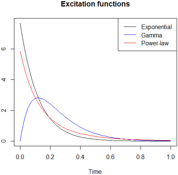
Excitation functions with respect to time : exponential (black), Gamma (blue), power-law (red)

As expected, an homogeneous Poisson process is not enough to model this type of event. We need to take into account the self-excitation property of the process. We could also see that the fitting is better with a Gamma excitation function than an exponential or a power-law decay, which validates our study a posteriori. We remark that the exponential and the power-law functions provide the same type of self-excitation with no delay, as we plot the fitted functions in Fig. 6.

Fig. 6.

Parameters used for Random Forest Regressor

Random Forest Regressor

In order to catch the temporal dependency of the natural disasters, we compare with a time series approach. We present here the results given by Random Forest Regressor (see Breiman and Forests (2001) for details about Random Forest), which fitted better that other types of time series models in terms of Kolmogorov-Smirnov test (ARIMA, ARMA, GARCH, Prophet). We used the scikit-learn estimator sklearn.ensemble.RandomForestRegressor and the parameters presented in Fig. 6.

We learned the time series from January 2015 to June 2019 and we predicted the number of events over 100 days from July 2019. Figures 7 and 8 shows the prediction (in blue) versus the real data (in orange, the peak corresponds to the tornado in August 2019).

Fig. 7.

Prediction of the time series by a Random Forest Regressor

Fig. 8.

Prediction of the time series by a Random Forest Regressor

We then compared the distribution of the interarrival times of the prediction with the distribution of the interarrival times of the actual time series with a QQ-plot in Fig. 9.

Fig. 9.

Simulation of 20 trajectories over five years for set of parameters estimated by EM algorithm

We could see that this approach does not allow to catch the severe peaks which characterize this time series. This kind of approach is more efficient on data with seasonality and a regular trend.

Simulations

Moreover, we must make sure that our model is able to replicate severe events like those observed in our data. We verify that simulated trajectories present the same structure than the actual time series: few severe events between very calm periods. Figure 10 shows the simulation of 20 trajectories over five years according to our estimated Hawkes process.

Fig. 10.

Simulation of 20 trajectories over five years for four set of parameters

Most of the simulated trajectories do not present the expected step function structure, observed with real insurance data. The evolution of the process counting is too smooth for these simulations, if we compare the dynamics between Figs. 3 and 6.

Let us see what happens with another set of parameters. Since the expectation of the process assuming stationarity is proportional to $\frac{{\lambda }^{\text{ND}}}{1-{\alpha }^{\text{ND}}}$, we slighty change ${\lambda }^{\text{ND}}$ and ${\alpha }^{\text{ND}}$ so that stationary expectation remains the same. Moreover, as we would like to have larger jumps in the trajectory, it means that the importance of the self-exciting part of the process should be higher. Thus, we will increase the value of ${\alpha }^{\text{ND}}$. We propose the same type of simulation over five years for different sets of $({\lambda }^{\text{ND}},{\alpha }^{\text{ND}})$ in Fig. 11.

Fig. 11.

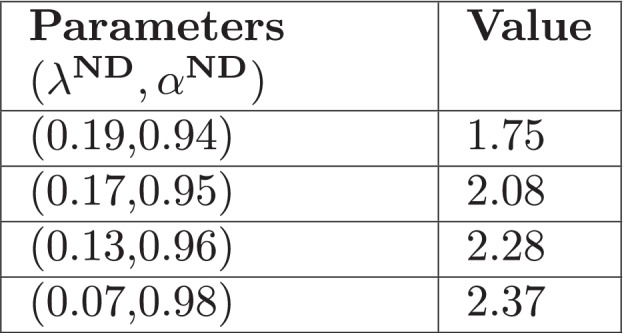
Average number of times the process reaches a threshold of 500 events in a period of time of 1825 days

Results show that increasing ${\alpha }^{\text{ND}}$ allows indeed the process to be more volatile and with more severe events. Simulated trajectories are more alike actual data for the different sets of parameters. The higher is ${\alpha }^{\text{ND}}$, the larger are the jumps. In order to quantify the capacity to generate scenarios with severe events, we evaluate by a Monte-Carlo method the average number of times the process reaches a threshold of 500 events in a period of time of 1825 days (five years), by performing 1000 simulations. We present the results on Fig. 12.

Fig. 12.

QQ-plot and Kolmogorov-Smirnov test for four set of parameters

The Monte-Carlo estimation shows that the higher is $\alpha$, the higher is the average value of severe events. Therefore it confirms that another set of parameters could be more appropriate in terms of ability to generate disasters observed on real data.

In terms of goodness-of-fit, Fig. 13 shows QQ-plot for each set of parameters.

Fig. 13.

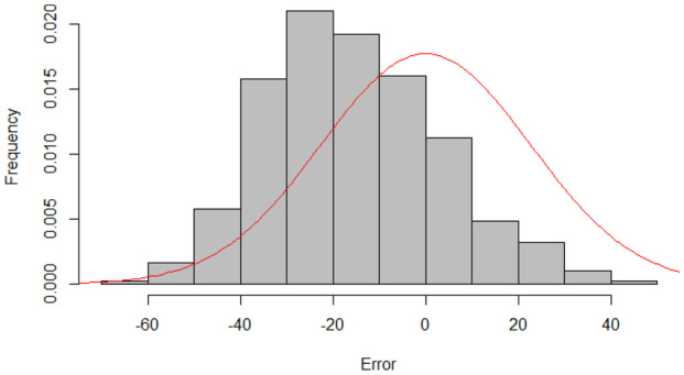
Distribution of errors at the end of the five years

Figure 13 illustrates that goodness-of-fit is worse for each set of parameters, when comparing to the first set of parameters we estimated by our approach (see Fig. 4). Indeed, for each set of parameters we could reject the hypothesis that the Hawkes process fits the data. We eventually have a set of parameters which maximizes the goodness-of-fit (the one estimated by the EM algorithm), but another which seems to catch better the dynamics of the time series (a set with a higher ${\alpha }^{\text{ND}}$). It is explained by the fact that the goodness-of-fit is evaluated on the entire distribution, by computing the distance on all the quantiles of the distribution. Whereas the dynamics of the natural disasters rely on the accumulation of grouped events, which are the smallest quantiles of the distribution. By the way we could see on Fig. 13 that the distribution gets worse on medium quantiles. There is an imbalance between the quality of simulations and the statistical tests, which illustrates the difficulty to estimate the right set of parameters for a Hawkes process.

Distribution of the Number of Events

In this subsection, we observe the distribution of N(t), where t = five years. We perform 1000 simulations of the Hawkes processes, with the first set of parameters estimated, for a time period of five years. We observe the errors distribution in Fig. 14, $\frac{N(t)-\overline{\lambda }t}{\sqrt{t}}$, and we compare with a Normal distribution of variance ${\sigma }^2=\frac{\lambda }{{(1-\alpha )}^3}t$.

Fig. 14.

A realisation of a Hawkes process and its branching structure

We see that the mean of errors is different from zero. The distribution of errors does not follow the Normal distribution, as the process is not observed long enough to be close to its limit. This observation justifies our mathematical study a posteriori, since the study of limits is not enough. We need the transitory values of the expectation and the variance, even for a long five years period.

Numerically, from Eqs. (10) and (13) we obtain:

$$\begin{array}{cc}\hfill \mathbb{E}(N(t))& =-655.55+3.25t-0.28exp(-0.22t)+655.84exp(-0.004t),\hfill \\ \hfill \mathbb{V}(N(t))& =-82154.94+383.66t-6.01exp(-0.22t)+82160.95exp(-0.004t),\hfill \end{array}$$ 17

with t in days.

The following table presents the observed, calculated and limit value of expectation and variance at the final time of simulations.

This table confirms that calculated expectation and variance give the correct values and that focusing on limits is not sufficient to study a process over several years, which is a quite long period for insurance use cases. Thanks to numeric values provided by Eqs. (23) and (24), we could see that we are still in either the transient state or the intermediary state for $t=5$ years $=1825$ days: while exponential terms are close to zero for both expectation and variance, the difference between the actual value (third column of Table 3) and the limit value (fourth column) is explained by the constant terms. The order of magnitude of these constant terms shows that the limit values are not a good approximation for a period of several years. That justifies our study on the different regimes.

Table 3.

Observed, calculated and limit value of expectation and variance

Quantity	Observed value	Calculated value	Limit value: linear term
Expectation	5265.2	5275.8	5931.2
Variance	621988.3	618039.4	700177.6

Conclusion and Future Work

In this paper, we introduced a complete framework for the study of Hawkes process: definition, estimation and simulation. We presented a specific form of Hawkes processes, the $\mathrm{\Gamma }$-Hawkes process, and we developed mathematical properties for this category of process. We applied this model to an insurance use case, i.e. natural disasters, and we observed that the considered Hawkes process is well fitted with historical data.

For future work, we intend to apply this model to other insurance use cases, such that:

• Life events prediction: births, marriage, job change, etc. We could use a multi-variate version of Hawkes processes (see Laub et al. (2015)), since one type of event could trigger another (e.g. a marriage could lead to a birth);

• Epidemic: we already studied the dynamics of Covid-19 pandemic in Lesage (2020). We intend to adapt the study to a long class of diseases;

• Workload prediction: we would like to anticipate peaks of workload for Foyer Assurances employees in order to optimize staffing.

Appendix

Appendix 1

Proof of the Proposition 2.

1. Laplace transform of $g(t)=\mathbb{E}[{\lambda }^{\ast }(t)]$ Since $\mathbb{E}(N(t))={\int }_0^t\mathbb{E}[{\lambda }^{\ast }(t)]dt$, we first focus on $\mathbb{E}[{\lambda }^{\ast }(t)]$, that we denote g(t). We saw that:

   $$\begin{array}{c}\hfill g(t)=\lambda +{\int }_0^t\mu (t-u)g(u)du.\end{array}$$ 18

   We recognize a convolution product of g and $\mu$, denoted $g\ast \mu$. Therefore it is much easier to work into Laplace domain, since $\mathcal{L}[g\ast \mu (t)](s)=\mathcal{L}[g(t)](s)\times \mathcal{L}[\mu (t)](s)$. By transforming Eq. (25) into Laplace domain:

   $$\begin{array}{cc}\hfill \mathcal{L}[g(t)](s)& =\mathcal{L}[\lambda +{\int }_0^t\mu (t-u)g(u)du](s)\hfill \\ \hfill & =\mathcal{L}[\lambda ](s)+\mathcal{L}[\mu (t)](s)\times \mathcal{L}[g(t)](s).\hfill \end{array}$$
   By rearranging, we obtain:

   $$\begin{array}{c}\hfill \mathcal{L}[g(t)](s)=\frac{\mathcal{L}[\lambda ](s)}{1-\mathcal{L}[\mu (t)](s)}.\end{array}$$ 19
2. Inverse of g(t) Laplace transform We turn the Laplace transform into the temporal domain. In our study, $\mu$ is a Gamma density function and is given by Eq. (3). We can show that the Laplace transform is (see D’Azzo and Houpis (1988)):

   $$\begin{array}{c}\hfill \mathcal{L}[\mu (t)](s)=\frac{\alpha }{{(1+k_{2}s)}^{k_1}}.\end{array}$$ 20
   By using Eq. (26) in Eq. (27), we obtain:

   $$\begin{array}{c}\hfill \mathcal{L}[g(t)](s)=\frac{\mathcal{L}[\lambda ](s)}{1-\mathcal{L}[\mu (t)](s)}=\frac{\lambda }{s(1-\frac{\alpha }{{(1+k_{2}s)}^{k_1}})}.\end{array}$$ 21

   • For $k_1$ = 1 (see Eq. (5)):

     $$\begin{array}{c}\hfill \mathcal{L}[g(t)](s)=\frac{\lambda }{s(1-\frac{\alpha }{(1+k_{2}s)})}=\frac{(\frac{\lambda }{1-\alpha })}{s}-\frac{(\frac{\alpha \lambda }{1-\alpha })}{\frac{1-\alpha }{k_2}+s}.\end{array}$$ 22
     By transforming Eq. (28) into the temporal domain, we obtain:

     $$\begin{array}{c}\hfill g(t)=\mathbb{E}({\lambda }^{\ast }(t))=\frac{\lambda }{1-\alpha }-\frac{\alpha \lambda }{1-\alpha }exp(-\frac{1-\alpha }{k_2}t).\end{array}$$ 23
   • For $k_1$ = 2 (see Eq. (4)):

     $$\begin{array}{c}\hfill \mathcal{L}[g(t)](s)=\frac{\lambda }{k_2^{2}s(\frac{1+\sqrt{\alpha }}{k_2}+s)(\frac{1-\sqrt{\alpha }}{k_2}+s)}+\frac{2\lambda }{k_2(\frac{1+\sqrt{\alpha }}{k_2}+s)(\frac{1-\sqrt{\alpha }}{k_2}+s)}\\ \hfill +\frac{\lambda s}{(\frac{1+\sqrt{\alpha }}{k_2}+s)(\frac{1-\sqrt{\alpha }}{k_2}+s)}.\end{array}$$ 24
     By turning Eq. (29) into the temporal domain, we obtain:

     $$\begin{array}{c}\hfill g(t)=\mathbb{E}(\lambda (t))=\frac{\lambda }{1-\alpha }+\frac{\lambda \sqrt{\alpha }}{2(1+\sqrt{\alpha })}exp(-\frac{1+\sqrt{\alpha }}{k_2}t)\end{array}$$ 25

     $$\begin{array}{c}\hfill -\frac{\lambda \sqrt{\alpha }}{2(1-\sqrt{\alpha })}exp(-\frac{1-\sqrt{\alpha }}{k_2}t).\end{array}$$ 26
   • For $k_1$ = 3 (see Eq. (4)):

     $$\begin{array}{c}\hfill \mathcal{L}[g(t)](s)=\frac{\lambda }{s(1-\frac{\alpha }{{(1+k_{2}s)}^3})}=\frac{\lambda }{s}+\frac{\lambda \alpha }{s({(1+k_{2}s)}^3-\alpha )}=\frac{\lambda }{s}+\frac{\lambda \alpha }{k_2^{3}s(s+\frac{1-{\alpha }^{1/3}}{k_2})(s^2+a_{1}s+a_2)}\end{array}$$ 27

     $$\begin{array}{c}\hfill =\frac{\lambda }{s}+\frac{\lambda \alpha }{k_2^3}[\frac{A}{s}+\frac{B}{s+r_1}+\frac{Cs+D}{{(s+a)}^2+{\omega }^2}]\text{by partial fraction decomposition, where:}\end{array}$$ 28

     $$\begin{array}{cc}\hfill r_1& =\frac{1-{\alpha }^{1/3}}{k_2},\hfill \\ \hfill a_1& =\frac{(2+{\alpha }^{1/3})}{k_2},\hfill \\ \hfill a_2& =\frac{(1-\alpha )}{(1-{\alpha }^{1/3})k_2^2},\hfill \\ \hfill a& =\frac{(2+{\alpha }^{1/3})}{2k_2},\hfill \\ \hfill \omega & =\frac{\sqrt{3}{\alpha }^{1/3}}{2k_2}.\hfill \end{array}$$ 29

     (A, B, C, D) is the solution of the following linear system:

     $$\left\{\begin{array}{cccccccccccc}& \hfill A& \hfill +& \hfill & \hfill B& \hfill +& \hfill & \hfill C& \hfill & \hfill & \hfill & \hfill =0\\ \hfill (a_1+r_1)& \hfill A& \hfill +& \hfill a_1& \hfill B& \hfill +& \hfill r_1& \hfill C& \hfill +& \hfill & \hfill D& \hfill =0\\ \hfill (a_2+r_1{a}_1)& \hfill A& \hfill +& \hfill a_2& \hfill B& \hfill & \hfill & \hfill & \hfill +& \hfill r_1& \hfill D& \hfill =0\\ \hfill r_1{a}_2& \hfill A& \hfill & \hfill & \hfill & \hfill & \hfill & \hfill & \hfill & \hfill & \hfill & \hfill =1\end{array}\right)$$
     The solution is:

     $$\begin{array}{cc}\hfill A& =\frac{1}{r_1{a}_2},\hfill \\ \hfill B& =\frac{1}{r_1(r_1{a}_1-r_1^2-a_2)},\hfill \\ \hfill C& =\frac{r_1-a_1}{a_2(r_1{a}_1-r_1^2-a_2)},\hfill \\ \hfill D& =\frac{r_1{a}_1-a_1^2+a_2}{a_2(r_1{a}_1-r_1^2-a_2)}.\hfill \end{array}$$ 30
     Therefore the Laplace transform equals:

     $$\begin{array}{c}\hfill \mathcal{L}[g(t)](s)=\frac{\lambda }{s}+\frac{\lambda \alpha }{k_2^3}[\frac{A}{s}+\frac{B}{s+r_1}+\frac{Cs+D}{{(s+a)}^2+{\omega }^2}]=\frac{\lambda }{s}+\frac{\lambda \alpha }{k_2^3}[\frac{A}{s}+\frac{B}{s+r_1}+\frac{C(s+a)}{{(s+a)}^2+{\omega }^2}+\frac{\frac{(D-Ca)}{\omega }\omega }{{(s+a)}^2+{\omega }^2}]\end{array}$$ 31

     $$\begin{array}{c}\hfill =\frac{\lambda }{(1-\alpha )s}+\frac{\lambda \alpha B}{k_2^3(s+r_1)}+\frac{\lambda \alpha C}{k_2^3}\frac{(s+a)}{{(s+a)}^2+{\omega }^2}+\frac{\lambda \alpha (D-Ca)}{k_2^3\omega }\frac{\omega }{{(s+a)}^2+{\omega }^2}\end{array}$$ 32

     By turning Eq. (31) into the temporal domain, we obtain:

     $$\begin{array}{c}\hfill g(t)=\mathbb{E}(\lambda (t))=\frac{\lambda }{1-\alpha }+\frac{\lambda \alpha B}{k_2^3}exp(-r_{1}t)+\frac{\lambda \alpha C}{k_2^3}cos(\omega t)exp(-at)+\frac{\lambda \alpha (D-Ca)}{k_2^3\omega }sin(\omega t)exp(-at).\end{array}$$ 33
3. Calculation of $\mathbb{E}(N(t))$ from g(t) From g(t), we calculate $\mathbb{E}(N(t))$:

   $$\begin{array}{c}\hfill \mathbb{E}(N(t))={\int }_0^{t}g(t)dt,\end{array}$$ 34

   which leads us to Eqs. (9), (10) and (11).

Appendix 2

Proof of the Proposition 3, inspired from Appendix A.2 of Laub et al. (2015).

1. Link between the variance and the covariance density $\mathrm{\Phi }(\tau )$ We calculate the variance from the so-called covariance density $\mathrm{\Phi }(\tau )$, $\tau >0$, defined in Hawkes (1971). According to Hawkes (1971), the covariance density is given by the following equation:

   $$\begin{array}{cc}\hfill \mathrm{\Phi }(\tau )& =\overline{\lambda }\mu (\tau )+{\int }_{-\infty }^{\tau }\mu (\tau -u)\mathrm{\Phi }(u)du\hfill \\ \hfill & =\overline{\lambda }\mu (\tau )+{\int }_0^{+\infty }\mu (\tau +u)\mathrm{\Phi }(u)du+{\int }_0^{\tau }\mu (\tau -u)\mathrm{\Phi }(u)du,\hfill \end{array}$$ 35

   where $\overline{\lambda }=\frac{\lambda }{1-\alpha }$. Considering the stationary Hawkes process $\tilde{N}(·)$, the variance $\mathbb{V}(\tilde{N}(t))$ and the covariance density are linked by the following equation:

   $$\begin{array}{c}\hfill \mathbb{V}(\tilde{N}(t))=\overline{\lambda }t+2{\int }_0^t{\int }_0^{t_1}\mathrm{\Phi }(t_2-t_1)d{t}_{1}d{t}_2.\end{array}$$ 36
2. Laplace transform of $\mathrm{\Phi }(\tau )$ We first calculate $\mathrm{\Phi }(\tau )$. We recognize a convolution product in Eq. (34). Thus we work in the Laplace domain:

   $$\begin{array}{c}\hfill \mathcal{L}[\mathrm{\Phi }(\tau )](s)=\mathcal{L}[\overline{\lambda }\mu (\tau )+{\int }_0^{+\infty }\mu (\tau +u)\mathrm{\Phi }(u)du+{\int }_0^{\tau }\mu (\tau -u)\mathrm{\Phi }(u)du](s)\end{array}$$ 37

   $$\begin{array}{c}\hfill =\overline{\lambda }\mathcal{L}[\mu (\tau )](s)+\underset{=:l_1(s)}{\underbrace{\mathcal{L}[{\int }_0^{+\infty }\mu (\tau +u)\mathrm{\Phi }(u)du](s)}}+\mathcal{L}[\mathrm{\Phi }(\tau )](s)\times \mathcal{L}[\mu (\tau )](s)\end{array}$$ 38

   For $k_1$ = 2:

   $$\begin{array}{cc}\hfill l_1(s)& =\mathcal{L}[{\int }_0^{+\infty }\mu (\tau +u)\mathrm{\Phi }(u)du](s)\hfill \\ \hfill & =\mathcal{L}[{\int }_0^{+\infty }\frac{\alpha (\tau +u)exp(-\frac{\tau +u}{k_2})}{k_2^2}\mathrm{\Phi }(u)du](s)\hfill \\ \hfill & =\mathcal{L}[{\int }_0^{+\infty }\frac{\alpha \tau exp(-\frac{\tau }{k_2})exp(-\frac{u}{k_2})}{k_2^2}\mathrm{\Phi }(u)du](s)\hfill \\ \hfill & +\mathcal{L}[{\int }_0^{+\infty }\frac{\alpha uexp(-\frac{\tau }{k_2})exp(-\frac{u}{k_2})}{k_2^2}\mathrm{\Phi }(u)du](s).\hfill \end{array}$$
   By using the definition of the Laplace transform:

   $$\begin{array}{cc}\hfill l_1(s)& =\frac{\alpha }{k_2^2}{\int }_0^{+\infty }\tau exp(-(s+\frac{1}{k_2})\tau )\underset{\mathcal{L}[\mathrm{\Phi }(\tau )](\frac{1}{k_2})}{\underbrace{[{\int }_0^{+\infty }exp(-\frac{u}{k_2})\mathrm{\Phi }(u)du]}}d\tau \hfill \\ \hfill & +\frac{\alpha }{k_2^2}{\int }_0^{+\infty }exp(-(s+\frac{1}{k_2})\tau )\underset{-\mathcal{L}[\mathrm{\Phi }(\tau ){]}^{\prime }(\frac{1}{k_2})}{\underbrace{[{\int }_0^{+\infty }uexp(-\frac{u}{k_2})\mathrm{\Phi }(u)du]}}d\tau \hfill \\ \hfill & =\frac{\alpha }{k_2^2(s+\frac{1}{k_2})}[\frac{1}{(s+\frac{1}{k_2})}\mathcal{L}[\mathrm{\Phi }(\tau )](\frac{1}{k_2})-\mathcal{L}[\mathrm{\Phi }(\tau ){]}^{\prime }(\frac{1}{k_2})].\hfill \end{array}$$
   By replacing $l_1(s)$ in Eq. (36) we obtain:

   $$\begin{array}{cc}\hfill \mathcal{L}[\mathrm{\Phi }(\tau )](s)& =\overline{\lambda }\mathcal{L}[\mu (\tau )](s)+\frac{\alpha }{k_2^2(s+\frac{1}{k_2})}[\frac{1}{(s+\frac{1}{k_2})}\mathcal{L}[\mathrm{\Phi }(\tau )](\frac{1}{k_2})-\mathcal{L}[\mathrm{\Phi }(\tau ){]}^{\prime }(\frac{1}{k_2})]\hfill \\ \hfill & +\mathcal{L}[\mathrm{\Phi }(\tau )](s)\times \mathcal{L}[\mu (\tau )](s).\hfill \end{array}$$ 39
   To solve Eq. (38) and find $\mathrm{\Phi }$, we need to calculate $\mathcal{L}[\mathrm{\Phi }(\tau )](\frac{1}{k_2})$ and $\mathcal{L}[\mathrm{\Phi }(\tau ){]}^{\prime }(\frac{1}{k_2})$. First, by substituting $s=\frac{1}{k_2}$ in Eq. (38), rearranging and using Eq. (27) for $\mathcal{L}[\mu (\tau )](s)$, we obtain:

   $$\begin{array}{c}\hfill \mathcal{L}[\mathrm{\Phi }(\tau ){]}^{\prime }(\frac{1}{k_2})+\frac{(2-\alpha )k_2}{\alpha }\mathcal{L}[\mathrm{\Phi }(\tau )](\frac{1}{k_2})=\frac{\overline{\lambda }{k}_2}{2}.\end{array}$$ 40
   Second, by differentiating Eq. (38), we obtain:

   $$\begin{array}{cc}\hfill \mathcal{L}[\mathrm{\Phi }(\tau ){]}^{\prime }(s)& =\overline{\lambda }\mathcal{L}[\mu (\tau ){]}^{\prime }(s)-\frac{2\alpha \mathcal{L}[\mathrm{\Phi }(\tau )](\frac{1}{k_2})}{k_2^2{(s+\frac{1}{k_2})}^3}+\frac{\alpha \mathcal{L}[\mathrm{\Phi }(\tau ){]}^{\prime }(\frac{1}{k_2})}{k_2^2{(s+\frac{1}{k_2})}^2}\hfill \\ \hfill & +\mathcal{L}[\mu (\tau ){]}^{\prime }(s)\mathcal{L}[\mathrm{\Phi }(\tau )](s)+\mathcal{L}[\mu (\tau )](s)\mathcal{L}[\mathrm{\Phi }(\tau ){]}^{\prime }(s).\hfill \end{array}$$ 41
   By substituting $s=\frac{1}{k_2}$ in Eq. (40), rearranging and using Eq. (27) for $\mathcal{L}[\mu (\tau )](s)$ and $\mathcal{L}[\mu (\tau ){]}^{\prime }(s)$, we obtain:

   $$\begin{array}{c}\hfill \mathcal{L}[\mathrm{\Phi }(\tau ){]}^{\prime }(\frac{1}{k_2})+\frac{\alpha k_2}{(2-\alpha )}\mathcal{L}[\mathrm{\Phi }(\tau )](\frac{1}{k_2})=\frac{-\overline{\lambda }{k}_2\alpha }{2(2-\alpha )}.\end{array}$$ 42
   Equations (39) and (41) form a system of two equations with two variables, $\mathcal{L}[\mathrm{\Phi }(\tau )](\frac{1}{k_2})$ and $\mathcal{L}[\mathrm{\Phi }(\tau ){]}^{\prime }(\frac{1}{k_2})$. Solving this system leads to:

   $$\begin{array}{c}\hfill \mathcal{L}[\mathrm{\Phi }(\tau )](\frac{1}{k_2})=\frac{\overline{\lambda }\alpha }{4(1-\alpha )},\\ \hfill \mathcal{L}[\mathrm{\Phi }(\tau ){]}^{\prime }(\frac{1}{k_2})=\frac{-\overline{\lambda }\alpha k_2}{4(1-\alpha )}.\end{array}$$ 43
   We can now solve Eq. (38). After rearranging:

   $$\begin{array}{cc}\hfill \mathcal{L}[\mathrm{\Phi }(\tau )](s)& =\frac{\alpha [\overline{\lambda }+\mathcal{L}[\mathrm{\Phi }(\tau )](\frac{1}{k_2})+\frac{\sqrt{\alpha }}{k_2}\mathcal{L}[\mathrm{\Phi }(\tau ){]}^{\prime }(\frac{1}{k_2})]}{k_2^2(s+\frac{1+\sqrt{\alpha }}{k_2})(s+\frac{1-\sqrt{\alpha }}{k_2})}-\frac{\alpha \mathcal{L}[\mathrm{\Phi }(\tau ){]}^{\prime }(\frac{1}{k_2})}{k_2^2(s+\frac{1-\sqrt{\alpha }}{k_2})}\hfill \\ \hfill & =\frac{-\sqrt{\alpha }[\overline{\lambda }+\mathcal{L}[\mathrm{\Phi }(\tau )](\frac{1}{k_2})+\frac{\sqrt{\alpha }}{k_2}\mathcal{L}[\mathrm{\Phi }(\tau ){]}^{\prime }(\frac{1}{k_2})]}{2k_2(s+\frac{1+\sqrt{\alpha }}{k_2})}\hfill \\ \hfill & +\frac{\sqrt{\alpha }[\overline{\lambda }+\mathcal{L}[\mathrm{\Phi }(\tau )](\frac{1}{k_2})-\frac{\sqrt{\alpha }}{k_2}\mathcal{L}[\mathrm{\Phi }(\tau ){]}^{\prime }(\frac{1}{k_2})]}{2k_2(s+\frac{1-\sqrt{\alpha }}{k_2})}.\hfill \end{array}$$ 44
3. Inverse Laplace transform of $\mathrm{\Phi }(\tau )$ We turn the Laplace transform of $\mathrm{\Phi }(\tau )$ into the temporal domain. For $k_1=2$, we can show that:

   $$\begin{array}{cc}\hfill \mathrm{\Phi }(\tau )& =D_{1}exp(-{\omega }_1\tau )+D_{2}exp(-{\omega }_2\tau ),\hfill \end{array}$$ 45

   where:

   $$\begin{array}{cc}\hfill {\omega }_1& =\frac{1+\sqrt{\alpha }}{k_2},\hfill \\ \hfill {\omega }_2& =\frac{1-\sqrt{\alpha }}{k_2},\hfill \\ \hfill D_1& =\frac{-\sqrt{\alpha }[\overline{\lambda }+\mathcal{L}[\mathrm{\Phi }(\tau )](\frac{1}{k_2})+\frac{\sqrt{\alpha }}{k_2}\mathcal{L}[\mathrm{\Phi }(\tau ){]}^{\prime }(\frac{1}{k_2})]}{2k_2}\hfill \\ \hfill & =\frac{-\sqrt{\alpha }\overline{\lambda }[4-3\alpha -\sqrt{\alpha }\alpha ]}{8k_2{(1-\alpha )}^2},\hfill \\ \hfill D_2& =\frac{\sqrt{\alpha }[\overline{\lambda }+\mathcal{L}[\mathrm{\Phi }(\tau )](\frac{1}{k_2})-\frac{\sqrt{\alpha }}{k_2}\mathcal{L}[\mathrm{\Phi }(\tau ){]}^{\prime }(\frac{1}{k_2})]}{2k_2}\hfill \\ \hfill & =\frac{\sqrt{\alpha }\overline{\lambda }[4-3\alpha +\sqrt{\alpha }\alpha ]}{8k_2{(1-\alpha )}^2}.\hfill \end{array}$$ 46

4. Calculation of $\mathbb{V}(\tilde{N}(t))$ from $\mathrm{\Phi }(\tau )$ From Eqs. (35) and (42), we calculate $\mathbb{V}(\tilde{N}(t))$.

$\square$  

Appendix 3

Simulaion is performed thanks to Ogata’s thinning algorithm. The idea of Ogata’s thinning algorithm is that randomly removing points from a “faster” simulated Poisson process (i.e. with a higher intensity function than targeted Hawkes process) allows to simulate a Hawkes process. This idea is based on the proposition below, which is inspired from Theorem 4.2 of Chen (2016):

We consider a point process, with conditional intensity function ${\lambda }^{\ast }(·)$. We also consider an upper-bound for ${\lambda }^{\ast }(·)$, $\overline{\lambda }\ge 0$, and a Poisson process $\overline{N}$ of parameter $\overline{\lambda }$ of jumping times ${\overline{T}}_i,i\ge 1$. Then the point process defined by:

$$\begin{array}{c}\hfill N(t)=\sum _{i\ge 1}{\mathbb{1}}_{\{{\overline{T}}_i\le t,U_i\le \frac{{\lambda }^{\ast }({\overline{T}}_i)}{\overline{\lambda }}\}},\end{array}$$ 47

where $(U_i)$ are i.i.d and follow an uniform distribution on [0, 1], is a process of conditional intensity function ${\lambda }^{\ast }(·)$.

A formulation of Ogata’s thinning algorithm is proposed in Laub et al. (2015) for instance. We notice that the use of a Gamma excitation function does not change the classic algorithm.

Appendix 4

We first present an interpretation of Hawkes processes introduced in Halpin and De Boeck (2013), useful to understand better the estimation algorithm. Events occurring in a Hawkes process could be seen as a population, which expands either by immigration or births. Immigrants correspond to occurrences due to the background intensity, which are spontaneous. Births correspond to occurrences due to the self-exciting part of the intensity, which are a consequence of the previous occurrences. We can consider that the Hawkes process is a sum of independent Poisson processes, where each occurrence would be a consequence of one of these Poisson processes:

$$\begin{array}{c}\hfill {\lambda }^{\ast }(t)=\lambda +\sum _{k=1}^{N(t)}\mu (t-t_k)=\sum _{i=0}^{N(t)}{\lambda }_i^{\ast }(t),\end{array}$$ 48

where ${\lambda }^{\ast }(·)$, $N(·)$ and $\mu (·)$ were introduced previously.

• The number of spontaneous occurrences is a Poisson process of rate $\lambda$ over $[0,\tau ]$, where $\tau \ge 0$ is the final time of observation. We denote ${\lambda }_0^{\ast }(t)=\lambda$;

• The number of responses to each event $t_i,i\ge 1$ is a Poisson process of rate $\mu (t-t_i)$ over $[t_i,\tau ]$. We denote ${\lambda }_i^{\ast }(t)=\alpha \mu (t-t_i)$.

Definition 7

(Process of Response). For each event $T_i$, we introduce the random variable $Z_i$, which indicates the process to which the event belongs.

As an example, we consider the realisation of a Hawkes process, represented in the Fig. 15.

• $Z_1=0$: event $T_1$ is a spontaneous occurrence.

• $Z_2=1$: event $T_2$ is a response to event $T_1$.

• $Z_3=1$: event $T_3$ is a response to event $T_1$.

• $Z_4=3$: event $T_4$ is a response to event $T_3$.

• $Z_5=0$: event $T_5$ is a spontaneous occurrence.

• And so on.

We could now detail a method to estimate parameters of Hawkes processes, developed in Halpin and De Boeck (2013) in particular. First, we define the likelihood of Hawkes processes.

Fig. 15.

Expectation for $k_1=1,k_2=9,\alpha =0.9,\lambda =0.3$

Definition 8

(Observations Likelihood). Let us consider $N(·)$ a point process of intensity function ${\lambda }^{\ast }(·)$, on time period $[0,\tau ]$, $\tau >0$. We denote $T=\{T_1,...,T_{N(\tau )}\}$ the jumping times until time $\tau$. We observe $N(\tau )=n$ and $T=\{t_1,..,t_n\}$. Observations log-likelihood $\ell (\{t_1,..,t_n\},\theta )$ of $N(·)$ is:

$$\begin{array}{c}\hfill \ell (\{t_1,..,t_n\},\theta )=\sum _{i=1}^{n}log({\lambda }^{\ast }(t_i))-{\int }_0^{\tau }{\lambda }^{\ast }(s)ds,\end{array}$$ 49

where $\theta$ is the set of parameters to estimate (i.e. $\lambda$ and parameters of the excitation function $\mu$).

Then we define the so-called complete likelihood, when assuming that $\{Z_1,...,Z_n\}$ introduced in Definition 7 are observed.

Definition 9

(Complete Likelihood). Assuming we observe $\{Z_1,...,Z_n\}=\{z_1,...,z_n\}$, then complete log-likelihood is:

$$\begin{array}{c}\hfill \ell (\{t_1,..,t_n\},\{z_1,z_2,...,z_n\},\theta )=\sum _{z=1}^n[\sum _{i=1}^{n}log({\lambda }_z^{\ast }(t_i)){\mathbb{1}}_{z_i=z}-{\mathrm{\Lambda }}_z(\tau )],\end{array}$$ 50

where ${\mathrm{\Lambda }}_z(\tau )={\int }_0^{\tau }{\lambda }_z^{\ast }(s)ds$. This complete likelihood allows us to build the Expectation-Maximization algorithm (or EM algorithm), which will estimate the parameters of Hawkes processes by minimizing this likelihood. We first define the quantity $Q(\theta |{\theta }^{{}^{\prime }})$ below.

Definition 10

We define:

$$\begin{array}{c}\hfill Q(\theta |{\theta }^{{}^{\prime }})=\mathbb{E}[l(\{t_1,..,t_n\},\{Z_1,...,Z_n\},\theta )|\{t_1,..,t_n\},{\theta }^{{}^{\prime }}],\end{array}$$ 51

where $\theta$ and ${\theta }^{\prime }$ are two sets of parameters and whose computation is the E step of the EM algorithm (see Proposition 6).

We can show that:

$$\begin{array}{cc}\hfill Q(\theta |{\theta }^{{}^{\prime }})& =\sum _{z=1}^n[\sum _{i=1}^{n}log({\lambda }_z^{\ast }(t_i))\mathbb{P}[Z_i=z|\{t_1,..,t_n\},{\theta }^{{}^{\prime }}]-{\mathrm{\Lambda }}_z(\tau )].\hfill \end{array}$$ 52

This Eq. (52) will be useful to describe the EM algorithm. This algorithm is based on the following proposition, which states that the iterative maximization of $Q(\theta |{\theta }^{{}^{\prime }})$ allows to converge to a local maximum of the complete likelihood. In other words, maximizing $Q(\theta |{\theta }^{{}^{\prime }})$ allows to estimate parameters (see Section 1.5 of McLachlan and Krishnan (1996) for the proof).

Proposition 6

The sequence defined by ${\theta }^{(m+1)}=\underset{\theta }{\text{argmax}}Q(\theta |{\theta }^{(m)})$ converges to a local maximum of $\ell (\{t_1,..,t_n\},\theta )$, the observations likelihood.

Then we write the EM algorithm:

1. Initialize $m=0$, ${\theta }^{(m)}={\theta }_0$

2. While convergence:

   • [E step] Compute $\mathbb{P}[Z_i=z|\{t_1,..,t_n\},{\theta }^{(m)}]$
   • [M step] Compute ${\theta }^{(m+1)}=\underset{\theta }{\text{argmax}}Q(\theta |{\theta }^{(m)})\to$ maximization by Nelder-Mead method (see Nelder (1965))
   • $m=m+1$.

To check the accuracy of the estimation, we simulate a Hawkes process over five years, we estimate the parameters and we compare estimation and actual parameters. We notice that the estimation is pretty accurate, except for the scale parameter $k_2$ but its impact is lower than the other parameters. Table 4 compares the two sets of parameters.

Table 4.

Comparison between actual and estimated parameters

Parameter	Actual value	Estimated value
$\lambda$	0.25	0.252
$\alpha$	0.9	0.986
$k_1$	1	1.172
$k_2$	5	6.836

Data availability Statement

The data that support the findings of this study, that is to say the occurrences of natural disasters claims for Foyer’s customers, are not openly available because they are the property of Foyer Assurances. Anonymous and incomplete data could be available from the authors upon reasonable request.

References

- Asmussen S (2003) Appl Prob Queues. 2003. Springer, Volume 51
- Bacry E, Delattre S, Hoffmann M, Muzy JF (2012) Scaling limits for Hawkes processes and application to financial statistics. arXiv: Probability
- Bacry E, Muzy JF (2014) Second order statistics characterization of Hawkes processes and non-parametric estimation. arXiv:1401.0903
- Bacry E, Mastromatteo I, Muzy JF (2015) Hawkes Processes in Finance. Market Microstructure and Liquidity 01(01)
- Bessy-Roland Y, Boumezoued A, Hillairet C (2020) Multivariate Hawkes process for cyber insurance. hal-02546343
- Bordenave C, Torrisi GL (2007) Large deviations of Poisson cluster processes. Stoch Models 23, 593–625
- Breiman L. Random Forests. Mach Learn. 2001;45:5–32. doi: 10.1023/A:1010933404324. [DOI] [Google Scholar]
- Chen Y (2016) Thinning Algorithms for Simulating Point Processes.
- Cheng Z, Seol Y. Diffusion Approximation of a Risk Model with Non-Stationary Hawkes Arrivals of Claims. Methodol Comput Appl Probab. 2020;22:555–571. doi: 10.1007/s11009-019-09722-8. [DOI] [Google Scholar]
- D'Azzo J, Houpis C (1988) Linear Control Systems Analysis and Design. McGraw-Hill Education (ISE Editions)
- Daley DJ, Vere-Jones D (2003) An Introduction to the Theory of Point Processes: Volume I: Elementary Theory and Methods. Springer, Volume 1
- Gao and Wang Functional central limit theorems and moderate deviations for Poisson cluster processes. Adv Appl Probab. 2020;52(3):916–941. doi: 10.1017/apr.2020.25. [DOI] [Google Scholar]
- Gao X, Zhu L. Functional central limit theorems for stationary Hawkes processes and application to infinite-server queues. Queueing Systems. 2018;90(1):161–206. doi: 10.1007/s11134-018-9570-5. [DOI] [Google Scholar]
- Halpin PF, De Boeck P (2013) Modelling Dyadic Interaction with Hawkes Processes. Psychometrika 78, 793-814 [DOI] [PubMed]
- https://statistiques.public.lu/en/news/territory/territory-climate/2019/10/20191001/index.html
- Hawkes AG (1971) Spectra of some self-exciting and mutually exciting point processes. Biometrika, vol. 58, pp. 83-90
- Laub PJ, Taimre T, Pollett PK (2015) Hawkes Processes. https://arxiv.org/abs/1507.02822
- Lesage L (2020) A Hawkes process to make aware people of the severity of COVID-19 outbreak: application to cases in France. https://hal.archives-ouvertes.fr/hal-02510642
- Ly A, Marsman M, Verhagen J, Grasman RP, Wagenmakers EJ (2017) A Tutorial on Fisher Information. https://arxiv.org/pdf/1705.01064.pdf
- McLachlan G, Krishnan T. The EM Algorithm and Extensions. New York: John Wiley and Sons; 1996. [Google Scholar]
- Mohler Short. Brantingham, Schoenberg, Self-Exciting Point Process Modeling of Crime. J Am Stat Assoc. 2011;106(493):100–108. doi: 10.1198/jasa.2011.ap09546. [DOI] [Google Scholar]
- Nelder JA, Mead R (1965) A Simplex Method for Function Minimization. Comp J 7(4):308-313
- Rasmussen JG (2018) Temporal Point Processes and the Conditional Intensity Function. arXiv:1806.00221v
Associated Data
This section collects any data citations, data availability statements, or supplementary materials included in this article.