Performance Evaluation of Parametric and Nonparametric Methods When Assessing Effect Measure Modification

Abstract

Effect measure modification is often evaluated using parametric models. These models, although efficient when correctly specified, make strong parametric assumptions. While nonparametric models avoid important functional form assumptions, they often require larger samples to achieve a given accuracy. We conducted a simulation study to evaluate performance tradeoffs between correctly specified parametric and nonparametric models to detect effect modification of a binary exposure by both binary and continuous modifiers. We evaluated generalized linear models and doubly robust (DR) estimators, with and without sample splitting. Continuous modifiers were modeled with cubic splines, fractional polynomials, and nonparametric DR-learner. For binary modifiers, generalized linear models showed the greatest power to detect effect modification, ranging from 0.42 to 1.00 in the worst and best scenario, respectively. Augmented inverse probability weighting had the lowest power, with an increase of 23% when using sample splitting. For continuous modifiers, the DR-learner was comparable to flexible parametric models in capturing quadratic and nonlinear monotonic functions. However, for nonlinear, nonmonotonic functions, the DR-learner had lower integrated bias than splines and fractional polynomials, with values of 141.3, 251.7, and 209.0, respectively. Our findings suggest comparable performance between nonparametric and correctly specified parametric models in evaluating effect modification.

Abbreviations:

AIPW

augmented inverse probability weighting

BMI

body mass index

DR

doubly robust

EAGeR

Effects of Aspirin on Gestation and Reproduction

EMM

effect measure modifier

GLM

generalized linear models

SD

standard deviation

SE

standard error

TMLE

targeted minimum loss-based estimation

 

Epidemiologists are often interested in evaluating whether exposure effects differ between individuals with certain clinical or demographic characteristics. Such questions about effect measure modification, while essential, are subject to several difficulties. For instance, a large proportion of studies in epidemiology are underpowered to detect effect modification simply because sample sizes are powered to detect main effects exclusively (1, 2). This holds true even when efficient parametric models (e.g., maximum likelihood estimation) are used. Additionally, to obtain unbiased (more technically, asymptotically consistent) estimators with appropriate confidence interval coverage, these parametric models must be correctly specified (1, 3–5). That is, researchers must accurately model the functional form of continuous modifiers and the interaction between covariates, as well as selecting appropriate family distributions and link functions. Unfortunately, scenarios in epidemiology are often too complex to confidently support strong parametric assumptions about the true underlying data-generating mechanisms with any degree of certainty.

In addition to concerns with power and model misspecification, categorizing continuous variables is also customary in effect measure modification analysis. For example, data from a recent randomized trial (6) were used to evaluate whether the effect of before-conception aspirin on live birth differed by body mass index (BMI, calculated as weight (kg)/height (m)²). To evaluate effect modification, women were categorized into normal weight (≤25) and overweight/obese (>25) BMI categories, and effects were estimated within strata of these categorized data (7). While this common approach is often implemented for reason of simplicity, it is well understood that such categorization results in loss of information and power, and underestimation of variability within levels of the categorical variables (8–11). Likewise, optimal threshold selection requires accurate background knowledge of the relationship between exposure, outcome, and the effect modifier. The lack of this substantive knowledge may lead researchers to choose “optimal” thresholds based on data dredging (8, 12). Furthermore, particularly when based on quantiles, these arbitrary cutpoints may not be relevant beyond the study’s sample (8).

Use of nonparametric methods, such as doubly robust (DR) machine learning–based estimators, is increasing in epidemiology. These methods avoid the need to rely on correct parametric model assumptions (13–19). However, while nonparametric methods make fewer assumptions about the true underlying data-generating mechanisms (such as the specific distribution that the outcome follows, or the functional form of the relation between the covariates and the outcome), they typically require much larger sample sizes to obtain a given level of accuracy (20, 21). The extent to which these losses materialize when effect measure modification is of primary interest is unknown. Furthermore, there are currently no empirical studies evaluating the performance of nonparametric methods to evaluate effect modification of a continuous effect modifier.

Here, we used simulated data to first evaluate the performance of nonparametric DR estimators to quantify effect measure modification across binary and continuous modifiers. Our aim was to evaluate the tradeoffs that result when using correctly specified parametric versus nonparametric methods. In the binary modifier case, we compared several parametric and nonparametric approaches and evaluated the impact of sample splitting when nonparametric approaches are used. In the continuous-modifier case, we compared flexible parametric approaches such as splines and fractional polynomials with their nonparametric counterpart, the DR-learner. Last, we built upon previous BMI analysis in the Effects of Aspirin on Gestation and Reproduction (EAGeR) Trial data to illustrate how these approaches can be used to evaluate effect modification. Specifically, we estimated the extent to which the effect of aspirin assignment on live birth is modified by BMI, using the continuous version of the BMI variable. We demonstrate how DR machine learning–based methods compare with flexible parametric approaches to estimate how the effect of low-dose aspirin on live birth changes as a function of BMI.

METHODS

Simulated data

Binary effect measure modifier.

To evaluate the performance of various methods to quantify the effect measure modifier (EMM), we devised 2 data-generating mechanisms. The first consisted of a continuous outcome, a binary exposure, a binary EMM, and 2 continuous confounders. The confounders ( and ) were drawn independently from a multivariate normal distribution with mean = 0 and standard deviation (SD) = 1. The exposure was then generated from a binomial distribution using a logistic regression model as:

(1)

where is the inverse of the logit function. An identical model was used to generate the binary EMM, which we denote M. Finally, the continuous outcome was obtained as:

(2)

where was randomly drawn from a normal distribution with mean equal to 0, and SD equal to 3 or 6. This outcome model yielded a mean difference between exposed and unexposed observations of 6 among those with and 3 among those with and . A total of 1,000 Monte Carlo simulations were performed, each with a sample of or .

Continuous effect measure modifier.

We used the same data-generating mechanisms to create the continuous confounders and binary exposure as described above. The continuous effect modifier was drawn from a uniform distribution, conditional on C and bounded between 0.1 and 13. The outcome was generated such that the mean difference for the exposure-outcome relationship varied as a function of the continuous effect modifier in 3 different scenarios. The first scenario (Figure 1A) was defined as a quadratic function using the following equation:

(3)

Figure 1.

True mean difference for the relationship between a binary treatment and a continuous modifier using 3 different functions: A) the quadratic function; B) the increasing monotonic function; C) the complex function.

The second scenario (Figure 1B) was defined as an increasing monotonic function:

(4)

Last, the third scenario (Figure 1C) was defined as a complex nonmonotonic relationship:

(5)

where is an indicator function that evaluates to 1 if the argument is true and 0 otherwise (22). For all the scenarios is drawn from a normal distribution with mean = 0 and SD = 6. These models generate a mean difference for the relationship between the binary exposure and continuous effect modifier that changes across the range of the effect modifier. The performance of methods for continuous effect modifiers was evaluated via 200 Monte Carlo simulations, each with a sample of n = 500.

Analysis

Binary effect measure modifier.

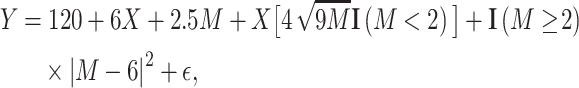
We used several techniques to analyze simulated data generated with a binary EMM. For each Monte Carlo sample, we fitted a correctly specified generalized linear model (GLM) with a Gaussian distribution and identity link that included a term for interaction between X and M, with the estimated effect in each M stratum obtained as a contrast of coefficients from the model (correct model). We also fitted 2 GLMs stratified by M to obtain a single coefficient for the exposure effect in each group. In our setting, this stratified modeling approach should be less efficient as it also (unnecessarily) allows all other coefficients in the model to vary between strata of M.

Two DR approaches, namely targeted minimum loss-based estimation (TMLE) and augmented inverse probability weighting (AIPW), were also used. TMLE is a maximum likelihood-based method that optimizes bias-variance tradeoffs on the parameter of interest by using an extra “targeting” step (13, 23). AIPW can be seen as “augmenting” the IPW estimator with an outcome model to fully utilize the information in the conditioning set (24, 25). These estimators (i.e., TMLE and AIPW) are asymptotically equivalent. Both TMLE and AIPW estimators were stratified by M. For TMLE, initial nonparametric machine learning (ML)-based models for the outcome and the exposure were fitted. Subsequently, a no-intercept logistic regression model for the outcome was generated, using the initial exposure model as weights (IPW), and the outcome model as an offset. Predictions from this “updated” model are generated by setting every individual to and then to . Finally, the effect in the given stratum M was obtained as follows:

(6)

where are the predictions from the updated model. For AIPW, we used predictions from the outcome model , as well as the propensity score from the exposure model to estimate the effect by M using the following equation:

(7)

Both estimators were fitted with and without 10-fold sample splitting (26), which proceeds by dividing the sample into roughly 10 equal folds. Models are then fitted in 9 of these folds, and the effect estimate is then computed in the remaining fold. This process is repeated 10 times, yielding 10 effect estimates for each stratum. The overall estimate is then obtained by averaging each of these 10 estimates.

DR estimators require specification of both the exposure and outcome models, which can both be estimated nonparametrically. We used a stacking algorithm (SuperLearner) for both that included: 1) random forests via the ranger package (500 trees with a minimum of 30 observations per node and 2 or 3 predictors sampled for splitting at each node); 2) generalized linear model via penalized maximum likelihood glmnet package with elastic-net mixing parameter from 0 to 1 by 0.2; 3) support vector machine via svm package with v = 0.25, 0.5, or 0.75, cost parameter = 1, and degree of polynomial = 3 or 4; 4) multivariate adaptive regression splines via earth package with degree of 2 and 3; 5) generalized additive models via gam package with 2, 3, and 4 knots; 6) Bayesian GLM via bayesglm package with normally distributed coefficient priors, mean = 0; 7) generalized linear models via glm package with identity link; 8) multinomial log-linear models via neural networks via nnet package; and 9) standard mean estimator via mean package (R Foundation for Statistical Computing, Vienna, Austria). Ten-fold cross-validation was used to estimate the weights for the SuperLearner (a process that is distinct from 10-fold sample splitting).

For each analytical approach, we computed the absolute bias, the mean standard error, and 95% confidence interval (CI) coverage. A measure of accuracy was defined as the ratio of the average of all standard errors divided by the standard deviation of all estimates. Relative efficiency was also calculated by taking the inverse of the ratio of the mean squared error (MSE) between the correctly specified GLM and each of the other estimators. These parameters were all calculated by M stratum, considering a true value of when and when . Power to detect EMM (i.e., interaction between X and M) was computed by testing whether the difference in the risk differences was different from zero using a Z-test. To do this, we estimated the pooled variance for the difference and calculated a 95% CI. Then, we computed the proportion of times that the 95% CI included the null.

In addition to the effect modification scenarios, we evaluated the performance of all our estimators for all the prespecified simulation conditions under no effect modification (i.e., interaction between X and M was set to zero). The results from these simulations is presented in the Web Table 1 (available at https://doi.org/10.1093/aje/kwab220). Additionally, we present the type I error rate for each estimator when testing for effect modification (see Web Table 2).

Continuous effect measure modifier.

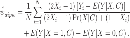
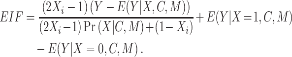
Continuous-modifier data were analyzed using 2 flexible parametric models, restricted cubic splines and second-degree fractional polynomials. These approaches have been used before to model interactions of treatment with continuous variables (12, 27, 28). Additionally, we used a DR influence function based estimator similar to AIPW, the DR-learner (29, 30). The DR-learner is a flexible, oracle efficient estimator, capable of providing model-free error bounds (29). This estimator was used to compute efficient influence function (EIF) values based on predictions from the outcome model and the propensity score model . The EIF was then computed as:

(8)

Intuitively, the EIF can be roughly interpreted as individual risk differences in the outcome. To estimate effect measure modification for the continuous effect modifier, we then regressed these EIF values against M using the SuperLearner algorithm with the same libraries described for the binary case. This regression step returns the risk difference for the outcome across the range of the continuous modifier. Finally, predictions from this SuperLearner are then plotted against the effect modifier values to obtain a risk difference values across the range of the continuous effect modifier. Using these predictions, we also computed integrated absolute bias (IAB) on a grid set across the range of EMM values with an increment of = 0.1, defined as:

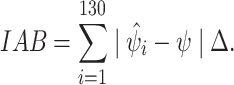(9)

And integrated squared bias (ISB), defined as:

(10)

In both cases, represents the mean estimated distribution of the 200 data sets derived from the Monte Carlo simulations, and the sum () is taken across the grid set.

Empirical data

To evaluate how nonparametric methods for continuous effect modification perform in a realistic data setting, we used data from 1,228 women in EAGeR (initiated in 2006 in multiple US states) to quantify the change in the effect of daily low-dose aspirin on livebirth as a function of continuous prepregnancy BMI. Details on the EAGeR data set are provided elsewhere (6). We sought to quantify the intent-to-treat effect of being assigned to receive 81 mg of aspirin per day () versus placebo (), adjusted for baseline level of high-sensitivity C-reactive protein. Prepregnancy BMI was the effect modifier, measured on a continuous scale. The outcome was an indicator of live birth status at the end of follow-up, which accrued for at most 6 menstrual cycles, and throughout pregnancy in those who became pregnant. EAGeR data were analyzed using restricted cubic splines, second-degree fractional polynomials, and the DR-learner.

RESULTS

The results from the binary case simulations are presented in Table 1. As expected, for all our simulations, the correctly specified GLM model that included an interaction term was unbiased in both EMM strata, with coverage ranging from 0.93 to 0.97. Similarly, the stratified GLM models were unbiased, with coverage of at least 0.95 in both EMM strata.

Table 1.

Performance of Different Estimators to Detect Effect Measurement Modification^a

Stratum and Estimator	Mean Bias	Mean SE	Coverage	Accuracy b	Relative Efficiency c
n = 200; SD = 3
Stratum 0 of the effect modifier
Interaction GLM	0.05	0.58	0.94	0.98	Referent
Stratified GLM	0.05	0.59	0.95	0.98	0.98
AIPW	0.10	1.09	0.99	1.59	0.36
AIPW with sample splitting	0.94	1.73	0.95	1.05	0.77
TMLE	0.26	0.94	0.96	1.09	0.40
TMLE with sample splitting	0.07	0.61	0.95	1.01	0.93
Stratum 1 of the effect modifier
Interaction GLM	0.01	0.64	0.93	0.90	Referent
Stratified GLM	0.01	0.73	0.95	1.00	0.80
AIPW	0.03	2.04	1.00	2.59	0.12
AIPW with sample splitting	0.04	1.06	0.96	1.05	0.57
TMLE	0.12	1.83	0.99	2.21	0.14
TMLE with sample splitting	0.02	0.76	0.94	1.01	0.76
n = 200; SD = 6
Stratum 0 of the effect modifier
Interaction GLM	0.10	1.16	0.94	0.98	Referent
Stratified GLM	0.10	1.17	0.95	0.98	0.98
AIPW	0.11	2.01	0.99	1.61	0.38
AIPW with sample splitting	2.32	3.92	0.95	1.04	0.77
TMLE	0.49	1.85	0.96	1.19	0.41
TMLE with sample splitting	0.14	1.22	0.94	1.01	0.93
Stratum 1 of the effect modifier
Interaction GLM	0.02	1.29	0.93	0.90	Referent
Stratified GLM	0.02	1.46	0.95	1.00	0.80
AIPW	0.08	3.87	1.00	2.51	0.13
AIPW with sample splitting	0.14	2.05	0.96	1.07	0.57
TMLE	0.22	3.63	0.99	2.23	0.14
TMLE with sample splitting	0.10	1.52	0.96	1.07	0.76
n = 500; SD = 3
Stratum 0 of the effect modifier
Interaction GLM	0.02	0.37	0.95	1.02	Referent
Stratified GLM	0.02	0.37	0.95	1.02	0.98
AIPW	0.02	0.69	0.99	1.54	0.34
AIPW with sample splitting	0.01	0.41	0.95	0.77	0.87
TMLE	0.25	0.60	0.93	0.63	0.38
TMLE with sample splitting	0.03	0.38	0.95	1.01	0.94
Stratum 1 of the effect modifier
Interaction GLM	0.02	0.41	0.94	0.96	Referent
Stratified GLM	0.01	0.46	0.97	1.06	0.8
AIPW	0.01	1.32	1.00	2.66	0.11
AIPW with sample splitting	0.01	0.51	0.98	0.99	0.69
TMLE	0.09	1.16	0.99	0.67	0.13
TMLE with sample splitting	0.01	0.47	0.96	1.05	0.77
n = 500; SD = 6
Stratum 0 of the effect modifier
Interaction GLM	0.03	0.73	0.95	1.00	Referent
Stratified GLM	0.03	0.74	0.95	1.02	0.98
AIPW	0.06	1.29	0.99	1.58	0.36
AIPW with sample splitting	0.05	0.8	0.95	0.98	0.87
TMLE	0.38	1.19	0.95	0.85	0.39
TMLE with sample splitting	0.06	0.76	0.95	1.01	0.94
Stratum 1 of the effect modifier
Interaction GLM	0.03	0.81	0.94	0.96	Referent
Stratified GLM	0.03	0.91	0.97	1.06	0.80
AIPW	0.04	2.51	1.00	2.58	0.12
AIPW with sample splitting	0.02	1.05	0.97	0.87	0.69
TMLE	0.24	2.30	0.99	1.81	0.13
TMLE with sample splitting	0.04	0.93	0.97	1.05	0.77

Abbreviations: AIPW, augmented inverse probability weighting; GLM, generalized linear model; MSE, mean squared error; SD, standard deviation; SE, standard error; TMLE, targeted minimum loss-based estimation.

^a Results from 1,000 Monte Carlo simulations.

^b Accuracy = average of SE()/SD().

^c [MSE(GLM)/MSE(estimator_i)]^–1.

The accuracy of the estimators was calculated as the ratio of the average standard error (SE) to the SD of the estimates from each Monte Carlo sample. This measure of accuracy captures how well the SE estimates the true sampling variation. In our experiment, the estimates () from each Monte Carlo simulation should follow a normal distribution, and the SEs associated with each simulation (i.e., SE()) should correspond to the standard deviation (i.e., SD()) of the distribution of estimates from all Monte Carlo simulations. Therefore, . An illustration of the relationship between the numerator (i.e., average SE() and the denominator (i.e., SD()) used for accuracy calculations can be found in the Web Figures 1–4. Under this definition, both GLM and stratified GLM were fully accurate (i.e., ).

Results from DR estimators for the binary modifier are presented in Table 1 and differed from the parametric case in several aspects. First, in all the scenarios we explored, these estimators showed slightly larger bias and mean squared error compared with its parametric counterparts. However, they showed better performance in terms of coverage. Accuracy of DR estimators was close to parametric models, but only when sample splitting was used, which underscores the importance of implementing this or alternative techniques to mitigate overfitting. For instance, in the scenario of and , the accuracy of TMLE went from 0.85 to 1.01 and from 1.81 to 1.05 in EMM stratum 0 and 1, respectively. AIPW showed a similar improvement going from 1.58 to 0.98 and from 2.58 to 0.87 in EMM stratum 0 and 1, respectively. A similar pattern was seen in all the additional scenarios.

The power to detect effect measure modification in all the scenarios is presented in Table 2. As expected, the greatest power for all our estimators was observed in the scenario where and . Overall, the GLM with an interaction term achieved the greatest power compared with all other estimators, ranging from 42% to 100% for the worst and best scenario, respectively. For AIPW, we observed improvements in power when sample splitting was used, regardless of the explored scenario. However, we did not observe any improvements in TMLE when sample splitting was used.

Table 2.

Power^a to Detect Effect Measure Modification by Several Estimators

Estimator	n = 200		n = 500
	SD = 3	SD = 6	SD = 3	SD = 6
GLM	0.93	0.42	1.00	0.77
AIPW	0.58	0.30	0.82	0.58
AIPW with sample splitting	0.79	0.34	0.99	0.70
TMLE	0.90	0.41	0.99	0.73
TMLE with sample splitting	0.90	0.38	0.99	0.76

Abbreviations: AIPW, augmented inverse probability weighting; GLM, generalized linear model; SD, standard deviation; TMLE, targeted minimum loss-based estimation.

^a Power to detect effect measure modification was computed by testing whether the difference in the risk differences was different from zero using a Z-test.

Figure 2 shows the conditional mean difference, , plotted against the range of the continuous modifier. The solid black line in each panel represents the true mean difference across the values of effect modifier as defined by the quadratic (Figure 2A–C), increasing monotonic (Figure 2D–F), and complex (Figure 2G–I) functions—models 4, 5, and 6, respectively.

Figure 2.

Estimation of continuous effect measurement modification with 2 flexible parametric models versus nonparametric doubly robust (DR)-learner estimator. Results from 200 Monte Carlo simulations of n = 500. True mean difference (solid black line) for a given function (dashed line) is presented across rows: quadratic (A, B, C); increasing monotonic (D, E, F); nonlinear, nonmonotonic (G, H, I). Results from a given model are presented by column: GLM with restricted cubic splines (A, D, G); second-degree fractional polynomial (B, E, H); DR-learner estimator (C, F, I). Individual results from simulation appear as gray lines in the back of each panel. EMM, effect measure modifier.

As depicted, the GLM with restricted cubic splines, the fractional polynomial of second degree, and the DR-learner estimator were able to capture the true quadratic and increasing monotonic functions (Figure 2A–F). In these scenarios, the flexible parametric approaches had lower integrated bias and squared bias compared with the DR-learner (Table 3). Conversely, the DR-learner estimator demonstrated a greater capacity to model the complex function compared with the GLM model with restricted cubic splines and the fractional polynomials of second degree (Figure 2G–I). Indeed, the integrated absolute bias was 141.3, 251.7, and 209.0 for the DR-learner, GLM with splines, and fractional polynomial, respectively. Similarly, integrated square bias was 339.4, 786.8, and 742.8 for the DR-learner, GLM with splines, and fractional polynomial, respectively (Table 3).

Table 3.

Performance of Different Estimators to Detect Effect Measurement Modification of a Continuous Modifier

Function and Estimator	Integrated Absolute Bias a	Integrated Square Bias a
Quadratic function
Restricted cubic spline	13.1	2.0
Fractional polynomial (second degree)	24.3	7.6
DR-learner	64.4	62.2
Increasing monotonic function
Restricted cubic spline	18.6	5.0
Fractional polynomial (second degree)	29.4	14.7
DR-learner	31.8	22.1
Complex function
Restricted cubic spline	251.7	786.8
Fractional polynomial (second degree)	209.0	742.8
DR-learner	141.3	339.4

Abbreviation: DR, doubly robust.

^a Integrated absolute bias and integrated square bias were calculated as the difference between true value and the estimate over a grid set across the range of the continuous modifier with an increase of Δ = 0.1.

Finally, a comparison between the DR-learner and our 2 flexible parametric approaches is presented in Figure 3. This figure shows the conditional risk difference for the relationship between before-conception daily low-dose aspirin and the probability of live birth across the range of prepregnancy BMI values. The original distribution of BMI in the EAGeR population can be found in the Web Figure 5. In general, the DR-learner and the fractional polynomial of second degree behave relatively similarly across the entire range of BMI values. As for the GLM with restricted cubic splines, we observed a similar behavior to the other estimators for BMI levels ranging between 20 and 40, followed by a sharp decline after this point.

Figure 3.

Conditional mean difference for the effect of aspirin on livebirth across body mass index (BMI) values in the Effects of Aspirin on Gestation and Reproduction (EAGeR) Trial (initiated in 2006 in multiple US states) using flexible parametric versus nonparametric doubly-robust (DR)-learner estimator. Results from 50 bootstrap resamples of n = 1,228.

DISCUSSION

We have outlined and evaluated an alternative approach to quantify effect modification based on nonparametric, doubly robust estimators. These estimators offer some degree of protection against model misspecification, particularly that arising from an incorrect functional form (31). Such functional form assumptions typically include no confounder-confounder interactions or linear dose-response relationships between continuous covariates and the outcome. Nevertheless, they also tend to suffer from losses in efficiency when compared with correctly specified parametric models.

Mounting theoretical and empirical evidence is suggesting that causal effect estimation with machine learning methods should only be done via doubly robust estimators (19, 32). However, little is known about how well these methods perform when used to address questions about effect measure modification. In the simulated scenarios we explored, we found that machine learning methods with doubly robust estimators can perform comparatively well but only when sample splitting was used. The use of sample splitting can reduce problems that result from overfitting and increase the accuracy and robustness of inferences when machine learning methods are used (33, 34). Importantly, these results align with previous simulation studies that demonstrate the importance of sample splitting (32, 19).

The extension to the continuous effect modifier demonstrated clearer benefits for adopting nonparametric doubly robust estimators when compared with using flexible parametric models, especially when evaluating nonlinear nonmonotonic functions. In this scenario, we found a much smaller integrated absolute bias and integrated squared bias when the DR-learner was compared with restricted cubic splines and second-degree fractional polynomials. Again, these results reflect the degree of flexibility between parametric and nonparametric methods. While we could have increased the degree of flexibility of these parametric models, we opted to use specifications that are most commonly used in applied epidemiologic analyses (35, 36, 37). Additionally, at a certain level of increased flexibility, the concerns commonly invoked regarding the use of nonparametric methods (e.g., curse of dimensionality) would be important to consider.

To illustrate the application of these methods in EAGeR data, we evaluated the extent to which the effect of low-dose aspirin on live birth was modified by BMI. In contrast to previous studies (7), we describe a functional relationship between BMI and aspirin assignment, hence enabling us to observe the risk-difference change in live birth compared with pregnancy loss for aspirin assignment across the entire range of BMI values. Overall, the flexible parametric models and the DR-learner produced similar results. Women with BMI in the range of 20–40 had a beneficial effect of aspirin on live birth, followed by a steady decline at higher BMIs. This may be the result of a dilution of the aspirin effect as BMI increases, as was observed in other studies outside perinatal epidemiology (38, 39).

Generalized linear models are among the most commonly used regression models in the applied sciences. When correctly specified, few methods will outperform generalized linear models. Furthermore, in our simulations, optimal performance was obtained even under mild misspecification (i.e., when effect modification was estimated via stratified GLM). It is reassuring then, that the nonparametric estimators we explored performed as well as the GLM approaches, particularly when sample splitting was used. Furthermore, in certain settings (such as when the effect modifier was continuous, and the function defining effect measure modification was complex), the nonparametric methods we explored outperformed GLMs rather markedly.

However, as appealing as these methods are, several considerations should be addressed before use. First, there is currently a wide array of libraries that can be included in the stacking algorithm. The decision to include a given library must consider the research question as well as previous knowledge, if any, about the relationship between exposure, outcome, and effect modifier. It is advisable to have a good balance between traditional parametric and data-adaptive models in the final pool of libraries (22). Second, data-adaptive methods should be carefully tuned to yield optimal performance. Tuning can be achieved by including a wide array of diverse algorithms in a stacking library (as we did in our study) but also by including screening algorithms that select important variables and/or variable transformations from the covariate adjustment set. We did not explore the impact of varying the algorithms in the stacking library, nor did we include screening algorithms. Third, our results demonstrate the importance of sample splitting to obtain correct standard errors. In this study, we split our samples into 10 folds; however, other research has relied on different numbers of sample-splitting folds ranging from 2 to 10. The tradeoff between choosing a smaller versus larger number of sample-splitting folds is, to our knowledge, unexplored. Finally, in our simulation study of the continuous effect modifiers, as well as our evaluation of the effect of low-dose aspirin on the probability of live birth as a function of continuous BMI, we did not consider standard error estimation. At present, there is no viable method to accurately estimate standard errors for continuous functionals when machine learning methods are used.

In summary, although it is generally accepted that treatment effects vary according to sociodemographic and clinical characteristics, studies specifically designed to detect EMM are rarely encountered in epidemiologic literature. Our study shows the utility of nonparametric, doubly robust, machine learning–based methods to approach the effect modification. These estimators perform relatively well compared with parametric methods under correctly specified conditions. Losses in performance should be mitigated by using sample splitting or similar techniques that avoid overfitting. Furthermore, its use will enable the analyst to avoid relying on parametric assumptions and are preferable in conditions of limited sample size, like most of those involving effect measure modification.

REFERENCES

- 1. Greenland S. Basic problems in interaction assessment. Environ Health Perspect. 1993;101(suppl 4):59–66. [DOI] [PMC free article] [PubMed] [Google Scholar]
- 2. Rencher A, Schaalje B. Multiple regression: Estimation. In: Rencher A, Schaalje B, eds. Linear Models in Statistics. Hoboken, NJ: John Wiley & Sons, Ltd; 2007:137–184. [Google Scholar]
- 3. VanderWeele TJ, Knol MJ. A tutorial on interaction. Epidemiol Methods. 2014;3(1):33–72. [Google Scholar]
- 4. Lubin JH, Samet JM, Weinberg C. Design issues in epidemiologic studies of indoor exposure to rn and risk of lung cancer. Health Phys. 1990;59(6):807–817. [DOI] [PubMed] [Google Scholar]
- 5. Greenland S. Tests for interaction in epidemiologic studies: a review and a study of power. Stat Med. 1983;2(2):243–251. [DOI] [PubMed] [Google Scholar]
- 6. Schisterman EF, Silver RM, Perkins Neil J, et al. A randomised trial to evaluate the effects of low-dose aspirin in gestation and reproduction: design and baseline characteristics. Paediatr Perinat Epidemiol. 2013;27(6):598–609. [DOI] [PMC free article] [PubMed] [Google Scholar]
- 7. Sjaarda LA, Radin RG, Silver RM, et al. Preconception low-dose aspirin restores diminished pregnancy and live birth rates in women with low-grade inflammation: a secondary analysis of a randomized trial. J Clin Endocrinol Metab. 2017;102(5):1495–1504. [DOI] [PMC free article] [PubMed] [Google Scholar]
- 8. Altman DG, Lausen B, Sauerbrei W, et al. Dangers of using “optimal” cutpoints in the evaluation of prognostic factors. J Natl Cancer Inst. 1994;86(11):829–835. [DOI] [PubMed] [Google Scholar]
- 9. Royston P, Altman DG, Sauerbrei W. Dichotomizing continuous predictors in multiple regression: a bad idea. Stat Med. 2006;25(1):127–141. [DOI] [PubMed] [Google Scholar]
- 10. Altman DG, Royston P. The cost of dichotomising continuous variables. BMJ. 2006;332(7549):1080. [DOI] [PMC free article] [PubMed] [Google Scholar]
- 11. MacCallum RC, Zhang S, Preacher KJ, et al. On the practice of dichotomization of quantitative variables. Psychol Methods. 2002;7(1):19–40. [DOI] [PubMed] [Google Scholar]
- 12. Royston P, Sauerbrei W. A new approach to modelling interactions between treatment and continuous covariates in clinical trials by using fractional polynomials. Stat Med. 2004;23(16):2509–2525. [DOI] [PubMed] [Google Scholar]
- 13. Schuler MS, Rose S. Targeted maximum likelihood estimation for causal inference in observational studies. Am J Epidemiol. 2017;185(1):65–73. [DOI] [PubMed] [Google Scholar]
- 14. Funk MJ, Westreich D, Wiesen C, et al. Doubly robust estimation of causal effects. Am J Epidemiol. 2011;173(7):761–767. [DOI] [PMC free article] [PubMed] [Google Scholar]
- 15. Bang H, Robins JM. Doubly robust estimation in missing data and causal inference models. Biometrics. 2005;61(4):962–973. [DOI] [PubMed] [Google Scholar]
- 16. Kang JDY, Schafer JL. Demystifying double robustness: a comparison of alternative strategies for estimating a population mean from incomplete data. Stat Sci. 2007;22(4):523–539. [DOI] [PMC free article] [PubMed] [Google Scholar]
- 17. Robins J, Rotnitzky A. Semiparametric efficiency in multivariate regression models with missing data. J Am Stat Assoc. 1995;90(429):122–129. [Google Scholar]
- 18. Kennedy EH. Semiparametric theory and empirical processes in causal inference. In: He H, Wu P, Chen D-G(D), eds. Statistical Causal Inferences and Their Applications in Public Health Research. New York, NY: Springer International Publishing; 2016:141–167. [Google Scholar]
- 19. Naimi AI, Mishler AE, Kennedy EH. Challenges in obtaining valid causal effect estimates with machine learning algorithms [published online ahead of print]. Am J Epidemiol. ( 10.1093/aje/kwab201). [DOI] [PMC free article] [PubMed] [Google Scholar]
- 20. Ploeg T, Austin PC, Steyerberg EW. Modern modelling techniques are data hungry: a simulation study for predicting dichotomous endpoints. BMC Med Res Methodol. 2014;14(1):137. [DOI] [PMC free article] [PubMed] [Google Scholar]
- 21. Riley RD, Ensor J, Snell KIE, et al. Calculating the sample size required for developing a clinical prediction model. BMJ. 2020;368:m441. [DOI] [PubMed] [Google Scholar]
- 22. Naimi AI, Balzer LB. Stacked generalization: an introduction to super learning. Eur J Epidemiol. 2018;33(5):459–464. [DOI] [PMC free article] [PubMed] [Google Scholar]
- 23. Laan MJ, Rubin D. Targeted maximum likelihood learning. Int J Biostat. 2006;2(1):11. [Google Scholar]
- 24. Glynn AN, Quinn KM. An introduction to the augmented inverse propensity weighted estimator. Political Analysis. 2010;18(1):36–56. [Google Scholar]
- 25. Robins JM, Rotnitzky A, Zhao LP. Estimation of regression coefficients when some regressors are not always observed. J Am Stat Assoc. 1994;89(427):846–866. [Google Scholar]
- 26. Kravitz ES, Carroll RJ, Ruppert D. Sample splitting as an M-estimator with application to physical activity scoring [preprint]. arXiv. 2019. https://arxiv.org/abs/1908.03967. Accessed on August 11, 2021. [Google Scholar]
- 27. Royston P, Sauerbrei W. Interaction of treatment with a continuous variable: simulation study of significance level for several methods of analysis. Stat Med. 2013;32(22):3788–3803. [DOI] [PubMed] [Google Scholar]
- 28. Royston P, Sauerbrei W. Interaction of treatment with a continuous variable: simulation study of power for several methods of analysis. Stat Med. 2014;33(27):4695–4708. [DOI] [PubMed] [Google Scholar]
- 29. Kennedy EH. Optimal doubly robust estimation of heterogeneous causal effects [preprint]. arXiv. 2020. https://arxiv.org/abs/2004.14497. Accessed August 11, 2021. [Google Scholar]
- 30. Laan MJ, Luedtke AR. Targeted learning of an optimal dynamic treatment, and statistical inference for its mean outcome. UC Berkeley Division of Biostatistics Working Paper Series Working Paper 329. 2003. https://biostats.bepress.com/ucbbiostat/paper329/. Accessed September 20, 2021.
- 31. Keil AP, Mooney SJ, Jonsson Funk M, et al. Resolving an apparent paradox in doubly robust estimators. Am J Epidemiol. 2018;187(4):891–892. [DOI] [PMC free article] [PubMed] [Google Scholar]
- 32. Zivich PN, Breskin A. Machine learning for causal inference: on the use of cross-fit estimators. Epidemiology. 2021;32(3):393–401. [DOI] [PMC free article] [PubMed] [Google Scholar]
- 33. Rinaldo A, Wasserman L, G’Sell M. Bootstrapping and sample splitting for high-dimensional, assumption-lean inference. Ann Stat. 2019;47(6):3438–3469. [Google Scholar]
- 34. Kreif N., DiazOrdaz K.. Machine learning in policy evaluation: new tools for causal inference [preprint]. arXiv. 2019. https://arxiv.org/abs/1903.00402. Accessed August 11, 2021. [Google Scholar]
- 35. Howe CJ, Cole SR, Westreich DJ, et al. Splines for trend analysis and continuous confounder control. Epidemiology. 2011;22(6):874–875. [DOI] [PMC free article] [PubMed] [Google Scholar]
- 36. Harrell FE Jr, Lee KL, Pollock BG. Regression models in clinical studies: determining relationships between predictors and response. J Natl Cancer Inst. 1988;80(15):1198–1202. [DOI] [PubMed] [Google Scholar]
- 37. Greenland S. Dose-response and trend analysis in epidemiology: alternatives to categorical analysis. Epidemiology. 1995;6(4):356–365. [DOI] [PubMed] [Google Scholar]
- 38. Patrono C, Rocca B. Type 2 diabetes, obesity, and aspirin responsiveness. J Am Coll Cardiol. 2017;69(6):613–615. [DOI] [PubMed] [Google Scholar]
- 39. Rothwell PM, Cook NR, Gaziano JM, et al. Effects of aspirin on risks of vascular events and cancer according to bodyweight and dose: analysis of individual patient data from randomised trials. Lancet. 2018;392(10145):387–399. [DOI] [PMC free article] [PubMed] [Google Scholar]
Associated Data
This section collects any data citations, data availability statements, or supplementary materials included in this article.