The authors recently discovered that a software update caused our mechanical testing device to be mis-calibrated, with the result that a subset of our samples was unusable for analysis. We sincerely regret this turn of events. The distribution of unusable samples by anatomic region is I=2/4, N=1/4, S=0/3, T=2/5 (number of unusable samples/original number of samples). We have reanalyzed our data, excluding the unusable samples. The major outcomes of the paper are unaffected; however, there are some minor changes in the numerical values of the mechanical properties, with updated values being: matrix Young’s modulus E = 2.576[1.25, 3.526] kPa (median [min., max.]), Poisson’s ratio v = 0.230[0.038, 0.329], kinetic time-constant τ = 218[10, 999] sec, and hydraulic permeability k = 2.012 × 10⁻¹ [2.000 × 10⁻², 9.979 10−1] mm4/(N sec). When fitting the usable experimental data, we used the maximum experimental standard deviation for each region as the fitting criteria, rather than ½ of this value as before. Further, the inferior and temporal regions are now more compliant than previously reported, and we thus observe a difference between regions in their axial strain response (p < 0.001). The following figures and captions reflect the changes (underlining shows changed text; updated figures are shown).
Figure 1: The scale bar in panel F is 0.140 mm.
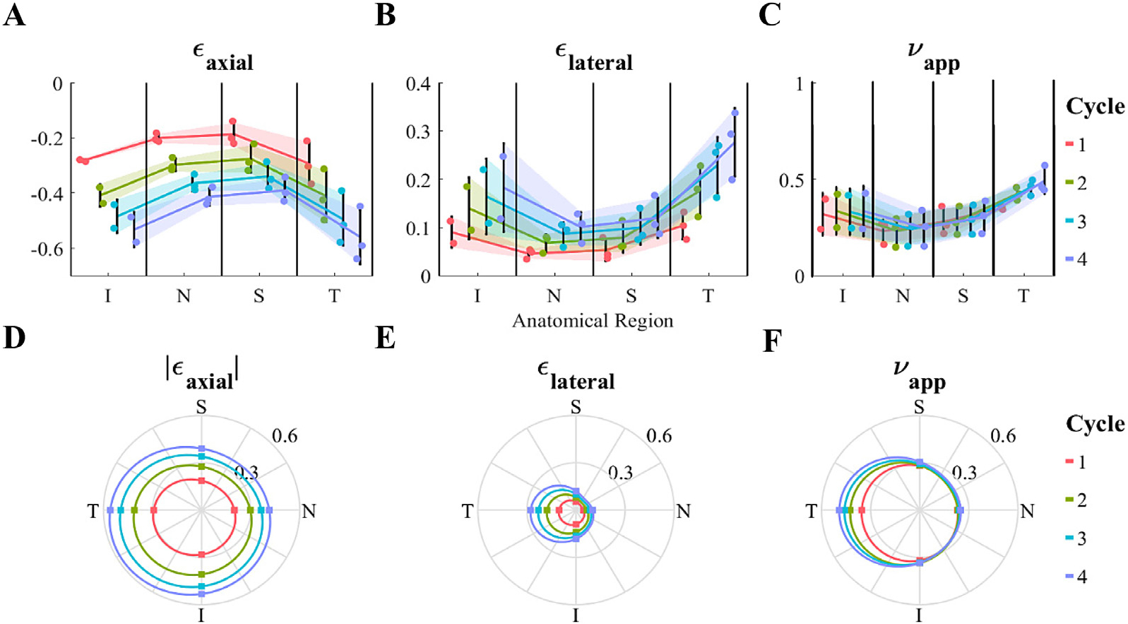
Fig. 2.

Regional dependence (analysis of variance) of (A and D) axial strain [∈axial], (B and E) lateral strain [∈lateral], and (C and F) apparent Poisson’s ratio [νapp]. For each parameter, the first row (A-C) shows the individual data points, their means ± standard deviation (shaded region) for each anatomical region and cycle number, and the second row (D-F) illustrates the mean values (dots) in a polar plot matching the anatomical orientations, where 0, 90, 180 and 270 degrees correspond to nasal [N], superior [S], temporal [T], and inferior [I], respectively. Each of ∈axial, ∈lateral and νapp were dependent on anatomical region, with the temporal and inferior quadrants being more compliant than the nasal and superior quadrants. The cycle number significantly impacted ∈axial and ∈lateral; however, it did not affect νapp. There was no interaction between the anatomical region and cycle number, i.e. heterogeneity was not affected by loading level.
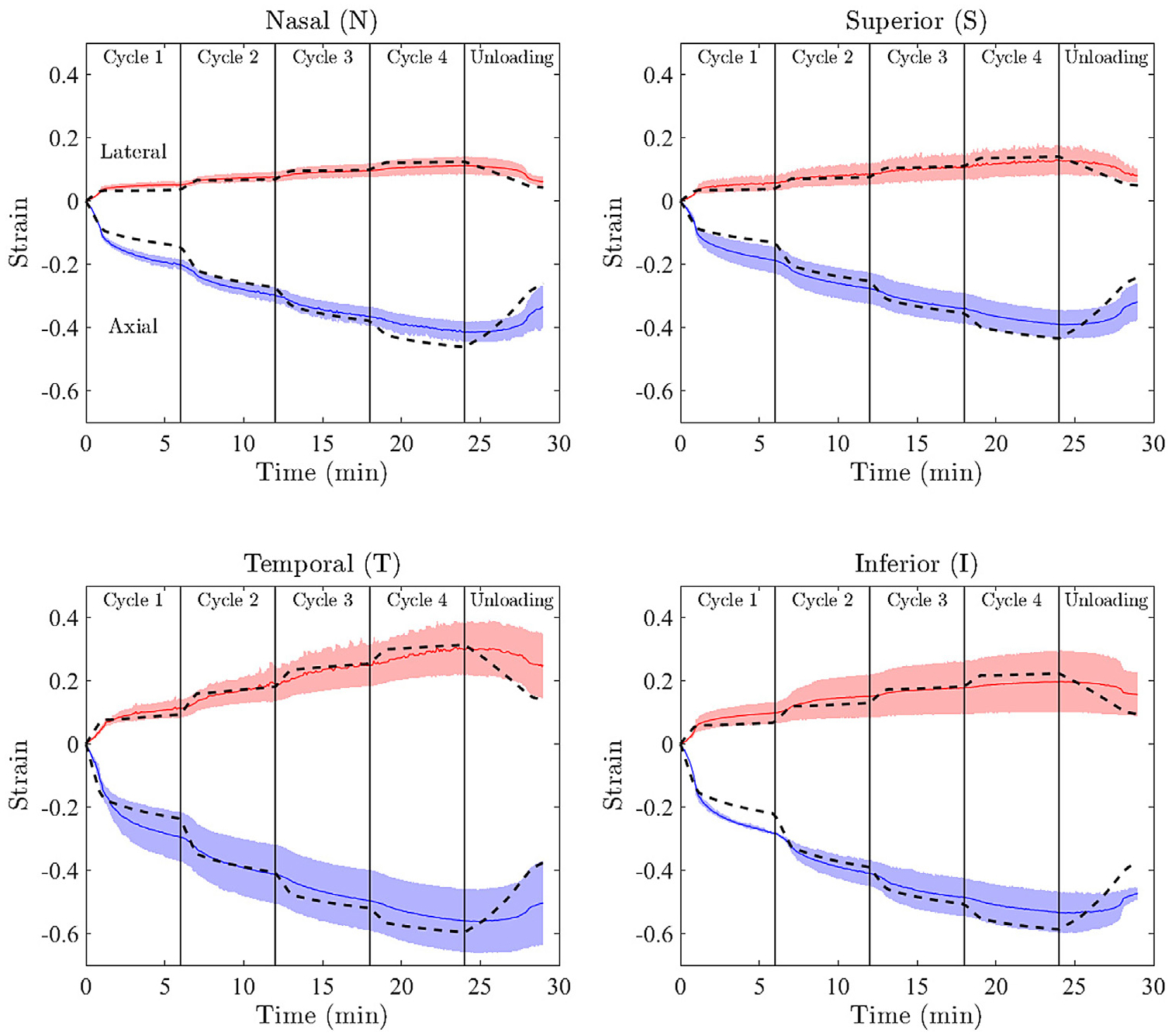
Fig. 3.

Results of data-fitting for each of the anatomical quadrants. The means ± standard deviation of the ex vivo experimental data are shown with solid lines and shading, respectively. Positive strains correspond to the lateral direction, while negative values are axial strains. For each region, the model response generated using the median of accepted fits is shown by the dashed lines. Note the good agreement between experimental (solid lines) and fitted (dashed lines) strains.
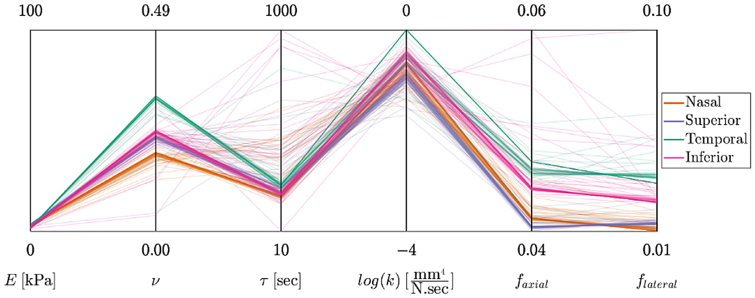
Fig. 4.

The data-fitting results shown in parallel coordinates format. The four coordinates on the left are the model parameters (E, ν, τ, k). For each model parameter, the graphed range of the coordinate corresponds to the prescribed range of model parameter values. The two additional coordinates are the RMSE of the fits in the axial and lateral direction (i.e., faxial and flateral).
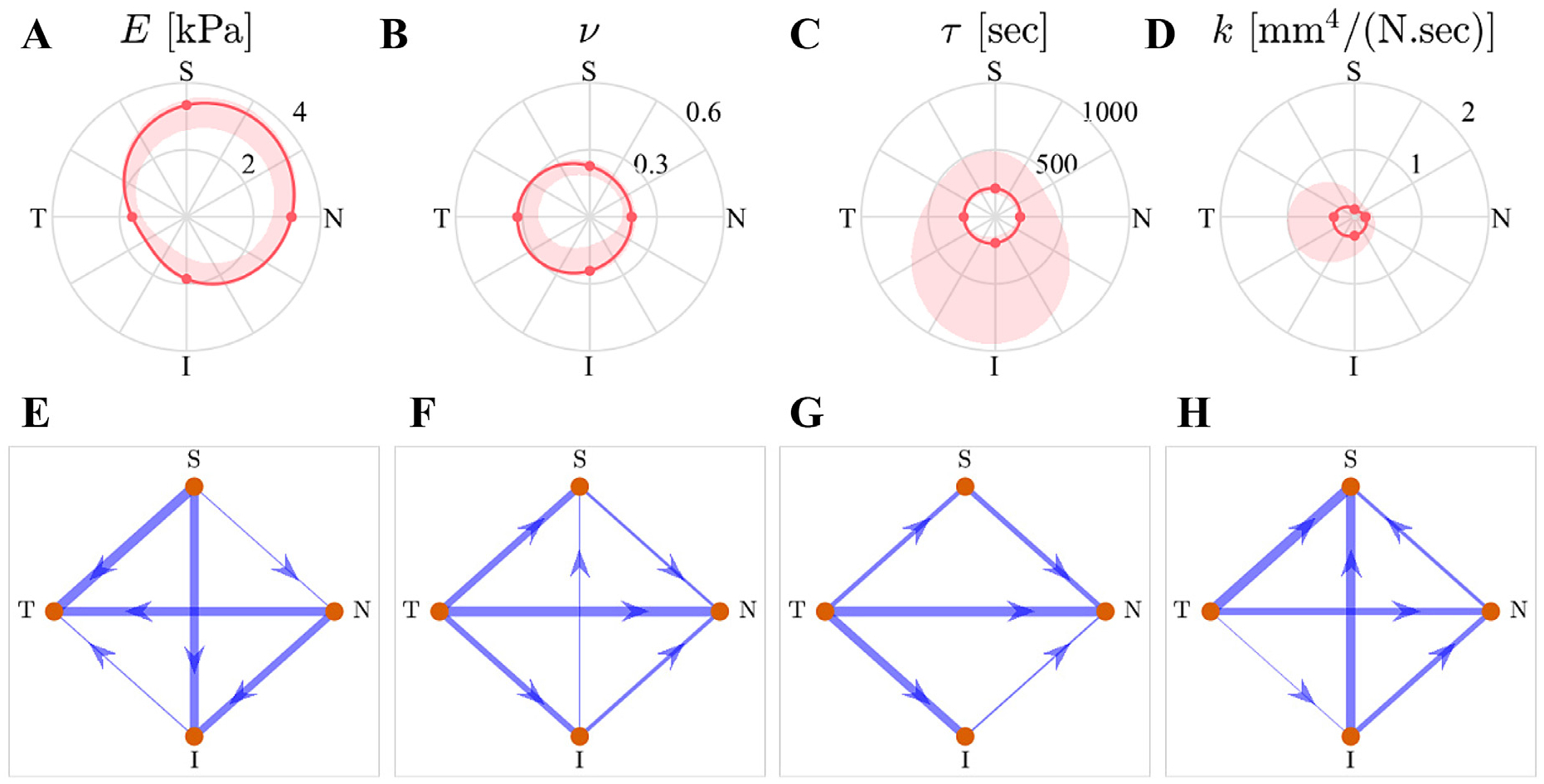
Fig. 5.

Anatomical distribution of the fit results. The first row shows the spatial distribution of each fit-ting parameter. The dots correspond to the median values, solid lines are the interpolated medians, and shaded areas are 95% confidence intervals for the acceptable fits (not the inter-sample variance). The second row shows the results of the multiple comparisons between the parameter values for each anatomical region using network graphs, where every arrow connecting two regions (start and destination) indicate that the “start” region has a statistically-significantly larger value compared to the “destination,” and the width of the lines is linearly proportional to the magnitude of the difference. The absence of a line implies that the difference was not statistically significant.


