Power calculation for analyses of cross-sectional stepped-wedge cluster randomized trials with binary outcomes via generalized estimating equations

Abstract

Power calculation for stepped-wedge cluster randomized trials (SW-CRTs) presents unique challenges, beyond those of standard parallel cluster randomized trials, due to the need to consider temporal within cluster correlations and background period effects. To date, power calculation methods specific to SW-CRTs have primarily been developed under a linear model. When the outcome is binary, the use of a linear model corresponds to assessing a prevalence difference; yet trial analysis often employs a nonlinear link function. We propose power calculation methods for cross-sectional SW-CRTs under a logistic model fitted by generalized estimating equations. Firstly, under an exchangeable correlation structure, we show the power based on a logistic model is lower than that from assuming a linear model in the absence of period effects. We then evaluate the impact of background prevalence changes over time on power. To allow the correlation among outcomes in the same cluster to change over time and with treatment status, we generalize the methods to more complex correlation structures. Our simulation studies demonstrate that the proposed power calculation methods perform well with the model-based variance under the true correlation structure and reveal that a working independence structure can result in substantial efficiency loss, while a working exchangeable structure performs well even when the underlying correlation structure deviates from exchangeable. An extension to our methods accounts for variable cluster sizes and reveals that unequal cluster sizes have a modest impact on power. We illustrate the approaches by application to a quality of care improvement trial for acute coronary syndrome.

1 ∣. INTRODUCTION

Stepped-wedge cluster randomized trials (SW-CRTs) have become increasingly popular in recent years.^1,2 In this type of design, clusters are randomized to cross-over from a control to an intervention condition in a sequential fashion (Table 1).³ In the first time-period, all clusters receive the control condition. At the beginning of each subsequent time-period, clusters are randomized to cross-over and initiate the intervention (the “steps”). By the final time-period, all clusters receive the intervention condition. The design offers a practical solution when the intervention can only feasibly be implemented in a few clusters at a given time. The design also has the advantage that all clusters will receive the intervention by the end of the trial, which may encourage community involvement.

TABLE 1.

Schematic of a balanced stepped-wedge cluster randomized trial (SW-CRT)

		Time-period
		1	2	3	4	5
Cluster	1	0	1	1	1	1
	2	0	1	1	1	1
	3	0	0	1	1	1
	4	0	0	1	1	1
	5	0	0	0	1	1
	6	0	0	0	1	1
	7	0	0	0	0	1
	8	0	0	0	0	1

Table 1 represents a SW-CRT with eight clusters (I = 8), four steps (I/q = 4), two clusters randomized to initiate the intervention at each step (q = 2), and five time-periods (T = I/q + 1 = 5). 0 represents control and 1 intervention.

Binary outcome measures are common in SW-CRTs.^4-6 Although power calculation has been extensively discussed for standard parallel cluster randomized trials (CRTs) with binary outcomes,^7-12 SW-CRT designs present unique challenges. Two notable features of the SW-CRT design are that: i) the outcome is measured within each cluster over time and ii) the treatment switches from the control to the intervention condition within a cluster at a particular time-period. These features give rise to more complex correlation structures than typically considered for standard parallel CRTs and also mean it is important to evaluate the role of background period effects on the estimated study power. We focus this article on the cross-sectional SW-CRT design, where the outcome is measured on different individuals within each cluster at each time-period. For example, in a cross-sectional SW-CRT to evaluate a hospital-based quality of care improvement intervention for acute coronary syndrome, the binary outcome of a cardiovascular event (yes/no) was measured among cross-sections of individuals attending the hospitals during each time-period.¹³

The majority of power calculation methods and software specific to SW-CRTs have been developed under a linear mixed-effects (LME) modeling framework.^14-17 Although a linear model is most suited to a continuous outcome, it has been applied in practice to calculate the power for a binary outcome where the intervention effect is on the prevalence difference scale. The assumption of a linear model is not ideal, since: i) the variance of a binary outcome is a function of the mean, hence it changes as the outcome probability changes and ii) the predicted outcome probability based on a linear model may be outside the (0, 1) range. Zhou et al¹⁸ considered a linear model with a truncated normal distribution to ensure the outcome probability fell within the (0, 1) range. Methods based on link functions other than the identity have not been extensively discussed for SW-CRTs,¹⁹ and are highlighted as an area for future development.¹⁷ In particular, for binary outcomes under a logit link function, we are aware of two power calculation publications; firstly, a method was developed by Li et al²⁰ under the generalized estimating equations (GEEs) approach, and secondly, a simulation-based method under a generalized linear mixed-effects model (GLMM) was investigated by Baio et al.²¹ Neither included a comparison to the power estimated if a linear model was assumed.

Furthermore, both the published approaches^20,21 focus on a few specific within-cluster correlation structures and assume equal cluster sizes. As previously mentioned, the SW-CRT design gives rise to more complex correlation structures. Additionally, while it is well known for standard parallel CRTs that cluster size variation reduces power,^8,11,12 the situation is more intricate for SW-CRTs. This is because in a SW-CRT the variance of the treatment effect estimator is dependent on when each variable size cluster initiates the intervention, which is determined by randomization.^22,23 Therefore, in this article, we address two important outstanding research questions:

1. Is estimating power of a cross-sectional SW-CRT with binary outcomes assuming an exchangeable correlation structure under a linear model based on testing the prevalence difference sufficient when a model implementing a logit link function will be fitted in the analysis phase?

2. How do more complex correlation structures and unequal cluster sizes impact the power of a cross-sectional SW-CRT with binary outcomes when a logit link function is utilized?

To address question one, we start this article by comparing the estimated power for binary outcomes based on detecting a prevalence difference under a LME model to that based on detecting a log odds ratio under a logistic model fitted by the GEE approach. To allow computation of a closed-form expression for the variance of the treatment effect estimate under the logistic model, we firstly simplify the standard mean model proposed by Hussey and Hughes¹⁴ based on an average treatment effect with discrete time-effects to the model in Zhou et al²⁴ that eliminates the time-effects. Under this simplified scenario, we show that the power when implementing a logistic model is lower than that realized with a linear model; something that has not previously been appreciated in the SW-CRT literature. We then explore power differences between the linear and logistic models with adjustment for discrete time-effects as in the standard mean model of Hussey and Hughes¹⁴ by numerically calculating the variance of the treatment effect estimate for the logistic model. This leads to an exploration of differences in study power under the logistic model as the outcome prevalence changes over time. Although it has been previously noted that power calculation with binary outcomes implicitly depends on the assumed period effect,²⁰ the dependence on outcome prevalence changes over time has not been explored in detail.

Subsequently, we address question two by extending the power calculation methods under the logistic model with discrete time-effects and the exchangeable correlation structure to three more complex correlation structures relevant to the cross-sectional SW-CRT design. To allow the correlation of outcomes within a cluster to change over time, we consider two structures. Firstly, the nested exchangeable correlation structure corresponding to the LME model of Hooper et al,²⁵ and Girling and Hemming,²⁶ which was also explored in Li et al²⁰ in the context of binary outcomes; and secondly the exponential decay correlation structure of Kasza et al.²⁷ To allow the correlation of outcomes within a cluster to change with treatment status, a heterogeneous treatment correlation structure inspired by Hughes et al²⁸ is explored. A method to calculate power for the exponential decay and heterogeneous treatment structures has not previously been published in the context of binary outcomes. Accounting for these more complex correlation structures can have a substantial impact on the estimated power. Lastly, since we know that under cluster size variation the power of a particular SW-CRT design is conditional on when each cluster is randomized to switch from the control to the intervention condition,^22,23 we extend the method proposed by Martin et al²² for the linear model to the logistic model to allow approximation of the mean, minimum and maximum power across randomization sequences. This analytical approach leads to an efficient power calculation method that would not be feasible by simulation as it would be too time-consuming to simulate scenarios across thousands of different randomization sequences as well as several complex correlation structures.

Previous attention had been paid to the performance of the GEE approach in finite samples in the context of SW-CRTs with logistic models.^20,29,30 To explore the number of clusters necessary for implementation of our power calculation technique, which is based on the model-based variance of the logistic model, we conducted a simulation study considering three variance estimates for the treatment effect in the analysis stage; i) the model-based variance, ii) the sandwich variance of Liang and Zeger,³¹ and iii) the bias-corrected sandwich variance of Mancl and DeRouen.³² Additionally, while implementing the GEE approach has the advantage of robustness to correlation misspecification via a sandwich variance, a recent simulation study under a linear model highlighted efficiency loss when adopting a working independence structure.³³ Therefore, we also explore the implications of adopting either a working exchangeable or independence structure along with a sandwich variance in the trial analysis stage; showing for the logistic model that adoption of a working exchangeable structure is adequate when there are 20 or more clusters but a working independence structure can result in efficiency loss.

We illustrate the power calculation methods described in this article by application to the quality of care improvement trial for acute coronary syndrome of Wu et al.¹³ This trial had a binary outcome measure and a logistic GEE approach was implemented in the analysis. Therefore, we retrospectively estimate study power both to illustrate our technique and to provide a real-life example of the impact of various design parameters on study power.

In summary, the main contributions of this article are firstly to elucidate differences in estimated power for cross-sectional SW-CRTs with binary outcomes under a logistic vs a linear model via a GEE approach, and secondly to provide methods to estimate power for this type of design under more complex correlation structures and variable cluster sizes. The article is structured as follows: Section 2.1 reviews the power calculation method based on the linear model of Hussey and Hughes.¹⁴ Section 2.2 compares the power calculated based on a linear model to that of a logistic model under no time-effect adjustment as well as discrete time-effect adjustment. Section 2.3 extends the power calculation method based on the logistic model with time-effect adjustment to more complex correlation structures. Considerations to take into account variable cluster sizes are in Section 2.4. The simulation study is in Section 3. Section 4 describes the illustrative example. We conclude with a Discussion (Section 5).

2 ∣. METHODS

2.1 ∣. Power calculation with a linear model

Following the landmark paper by Hussey and Hughes,¹⁴ several publications and widely used software^14-17,21 have the capability to perform power calculation based on an average treatment effect in the following linear random-intercepts model with discrete fixed time-effects:

$$Y_{ijk}={\beta }_j+X_{ij}\theta +{\alpha }_i+e_{ijk},{\alpha }_i\sim N(0,{\tau }^2),e_{ijk}\sim N(0,{\sigma }_e^2),$$ (1)

where Y_ijk is the outcome for individual k = 1, … , n at time-period j = 1, … , T in cluster i = 1, … , I for a cross-sectional design where different individuals are observed in each time-period. β_j is the fixed effect for jth time-period, X_ij is the treatment indicator of cluster i in period j (X_ij = 1 if cluster i receives intervention in period j and 0 otherwise), θ is the treatment effect, α_i is the random-effect for cluster i, and e_ijk is the individual-specific error independent of α_i. This model can be reformulated as a marginal model with an exchangeable correlation structure and identity link function, as follows:

$$\mathbb{E}(Y_{ijk}\mid X_{ij})={\beta }_j+X_{ij}\theta ,\text{var}(Y_{ijk})={\sigma }_e^2+{\tau }^2={\sigma }^2,\text{corr}(Y_{ijk},Y_{ij{k}^{\prime }})=\text{corr}(Y_{ijk},Y_{i{j}^{\prime }{k}^{\prime }})=\rho =\frac{{\tau }^2}{{\sigma }_e^2+{\tau }^2}=\frac{{\tau }^2}{{\sigma }^2}.$$ (2)

Although this model is primarily suited to continuous outcomes, it has often been used to estimate the power of a cross-sectional SW-CRT with binary outcomes where θ = p₁ − p₀ represents a prevalence difference in the outcome between intervention and control; with p₁ representing the outcome probability under intervention and p₀ the outcome probability under control. All software packages outlined in Table 2 will perform a power calculation based on this model following specification of p₁ and p₀ along with ρ the correlation between outcomes in the same cluster. The packages differ in their assumed values for ${\sigma }_e^2$ and τ².

TABLE 2.

Available software for power calculation for binary outcomes based on a linear model assessing a prevalence difference with discrete time-effect adjustment

Software	Optionsa	${\sigma }_{\mathit{e}}^2$	τ 2	Publication
R/excel, swCRTdesign::swPwr		$\frac{p_0+p_1}{2}\left(1-\frac{p_0+p_1}{2}\right)$	$\frac{\rho }{1-\rho }\left\{\frac{p_0+p_1}{2}\left(1-\frac{p_0+p_1}{2}\right)\right\}$	14,17
STATA, steppedwedge	Within	p0(1 – p0)	$\frac{\rho }{1-\rho }{p}_0(1-p_0)$	15,34
	Total	p0(1 – p0) – τ2	ρp0(1 – p0)
R, SWSamp::HH.binary	Within	$\frac{p_0(1-p_0)+p_1(1-p_1)}{2}$	$\frac{\rho }{1-\rho }\left\{\frac{p_0(1-p_0)+p_1(1-p_1)}{2}\right\}$	21
	Total	$\frac{p_0(1-p_0)+p_1(1-p_1)}{2}-{\tau }^2$	$\rho \left\{\frac{p_0(1-p_0)+p_1(1-p_1)}{2}\right\}$
R, Shiny CRT Calculator		$\frac{p_0(1-p_0)+p_1(1-p_1)}{2}-{\tau }^2$	$\rho \left\{\frac{p_0(1-p_0)+p_1(1-p_1)}{2}\right\}$	16

Note: p₀ = outcome probability under control, p₁ = outcome probability under intervention, ρ = intercluster correlation, ${\sigma }_e^2$ and τ² are as defined by Model (1).

^aOptions provided by the software package to calculate ${\sigma }_e^2$ and τ² from p₀, p₁, and ρ.

2.2 ∣. Comparison of power for a logistic vs a linear model

Models with a logit link function are frequently applied to analyze binary outcome data. Therefore, the implications of calculating study power based on a linear model when a logistic model will be utilized to analyze the trial is important.

For ease of a comparison, we firstly simplify Model (2) in Web Appendix A to SW-CRTs that take place over a relatively short time frame and do not require adjustment for a time trend.²⁴ Under this simplified scenario, a closed-form expression for the variance of the treatment effect estimate exists under both a linear and a logistic model. We determine that the Wald statistic of the treatment effect estimate based on a log odds ratio is lower than that based on a prevalence difference, and hence the approximate power to detect a treatment effect is lower for the logistic model than the linear model (Web Appendix A). The magnitude of the difference in estimated power is shown for p₀ = 0.1 and corresponding log odds ratios [θ* = logit(p₁) − logit(p₀)] when n = 30, ρ = 0.1, I = 20, and T = 5 in Figure 1A. At a log odds ratio of −0.39, corresponding to p₁ = 0.07, the estimated power based on the linear model is 80% and the estimated power based on the logistic model is lower at 76.1%. Web Figure 1 shows that the difference in estimated power increases substantially as ρ increases or n decreases for a control prevalence of p₀ = 0.1; whereas for a control prevalence of 0.5, ρ and n have little influence on the magnitude of the difference. Since models without time-effect adjustment are generally inadequate in practice, we next discuss models that include discrete time-effects.

FIGURE 1.

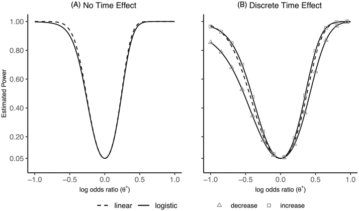
Comparison of estimated power for binary outcomes under the linear and logistic models. Panel A displays estimated power for the linear and logistic models with no time effect adjustment (Web Appendix A) for an outcome probability under control (p₀) of 0.1 and detectable log odds ratio [θ* = logit(p₁) – logit(p₀)] from −1 to 1. Panel B displays estimated power for the linear model with discrete time-effect adjustment [Model (2)] for an outcome probability under control (p₀) of 0.1 and detectable log odds ratio [θ* = logit(p₁) – logit(p₀)] from −1 to 1. Additionally, Panel B displays estimated power for the logistic model with discrete time-effect adjustment [Model (4)] for a detectable log odds ratio (θ*) from −1 to 1 and an outcome probability under control at the first time-period of 0.1, which either decreases (triangle) or increases (square) at each subsequent time-period by 0.01. Both figures are for a SW-CRT design with n = 30, ρ = 0.1, I = 20, and T = 5

In general, adjustment for time in SW-CRT analysis is recommended to avoid a biased intervention effect estimate. This is because the intervention status and time are correlated, so if time is associated with the outcome, the intervention effect will be confounded by time. When discrete time-effects are included in the linear model, as in Model (2), the variance of the treatment effect estimate has a closed-form expression.¹⁴ For balanced SW-CRT designs where q clusters are randomized to cross-over to intervention at each step and each cluster contributes n individuals at each time-period (Table 1), the expression is:

$$\text{var}(\widehat{\theta })=\frac{12{\sigma }^2(T-1)(1-\rho )(1-\rho +Tn\rho )}{nIT(T-2)\{2(1-\rho )+n\rho (T+1)\}}.$$ (3)

Due to the adjustment for discrete time-effects, the variance in Equation (3) is larger than that calculated in Web Appendix A for the linear model without time-effects; however, the expression does not depend on the magnitude of the time trend since β_j does not appear in Equation (3). As we will illustrate below, this is no longer the case when a logit link function is used.

When a logistic model with discrete time-effect adjustment is considered, we can write the model as:

$$\mathrm{logit}\{\mathbb{E}(Y_{ijk}\mid X_{ij})\}={\beta }_j^{\ast }+X_{ij}{\theta }^{\ast },Y_{ijk}\sim \text{ber}\{\mathbb{E}(Y_{ijk}\mid X_{ij})\},\text{corr}(Y_{ijk},Y_{ij{k}^{\prime }})=\text{corr}(Y_{ijk},Y_{i{j}^{\prime }{k}^{\prime }})=\rho ,$$ (4)

where ber represents the Bernoulli distribution. It is not possible to derive a closed-form expression for the variance of the treatment effect estimate under Model (4). However, the variance can be calculated by numerical matrix inversion:²⁰

$$\text{var}({\widehat{\theta }}^{\ast })={\left\{{\left(\sum _{i=1}^I{Z}_i^{⊺}{W}_i{Z}_i\right)}^{-1}\right\}}_{(T+1,T+1)},$$ (5)

where Z_i is the design matrix given by Z_i = (I_T,X_i) ⊗ 1_n with I_T the T × T identity matrix, X_i = (X_i1, … , X_iT)^⊺ is the treatment sequence for cluster i, ⊗ is the Kronecker product, 1_n is the vector of 1’s of length n, and W_i is the weight matrix given by $W_i=A_i^{1∕2}{R}_i^{-1}{A}_i^{1∕2}$ with $R_i^{-1}=\{(1-\rho )I_{nT}+\rho 1_{nT}{1}_{nT}^{⊺}{\}}^{-1}$, A_i = diag {p_i1(1 − p_i1), … , p_iT(1 − p_iT)} ⊗ I_n, $p_{ij}=\text{expit}({\beta }_j^{\ast }+{\theta }^{\ast }{X}_{ij})$. For example, for the SW-CRT given in Table 1, we have:

$$\begin{gathered} X_1=(0,1,1,1,1{)}^{⊺},X_2=(0,1,1,1,1{)}^{⊺},X_3=(0,0,1,1,1{)}^{⊺},X_4=(0,0,1,1,1{)}^{⊺}, \\ {X}_5=(0,0,0,1,1{)}^{⊺},X_6=(0,0,0,1,1{)}^{⊺},X_7=(0,0,0,0,1{)}^{⊺},X_8=(0,0,0,0,1{)}^{⊺}. \end{gathered}$$

As noted in Li et al,²⁰ $\text{var}({\widehat{\theta }}^{\ast })$ depends on the anticipated time trend since p_ij, the outcome probability at each time-period, is included in the W_i component of the variance of the treatment effect estimate in Equation (5). Therefore, the power to detect a fixed log odds ratio under the logistic model depends on changes in the outcome prevalence over time. If the outcome prevalence is less than 50% at the first time-period, then an increasing outcome prevalence under control during the SW-CRT will result in higher power. Whereas, if the outcome prevalence is greater than 50% at the first time-period, a decreasing outcome prevalence will result in higher power. This is because the power to detect a certain log odds ratio is highest at probabilities close to 0.5. For illustration on Figure 1B, we display the power based on the logistic model with discrete time-effect adjustment for detectable log odds ratio (θ*) from −1 to 1 with an outcome prevalence of 0.1 in the first time-period, decreasing or increasing by 0.01 at each subsequent time-period, as well as the power for the linear model with discrete time-effect adjustment.

2.3 ∣. More complex correlation structures

We extend the power calculation method based on the Wald test of the treatment effect under the logistic model with discrete time-effects, ${\mathrm{W}}_{\text{logistic}}=\mid {\theta }^{\ast }∕\surd \text{var}({\widehat{\theta }}^{\ast })\mid$, to three more complex correlation structures:

1. Firstly, the nested exchangeable correlation structure corresponding to the LME model in Hooper et al,²⁵ and Girling and Hemming,²⁶ which allows the correlation of outcome measures in the same cluster at the same time-period to differ from the correlation of outcome measures in the same cluster at different time-periods:

   $$\log \text{it}\{\mathbb{E}(Y_{ijk}\mid X_{ij})\}={\beta }_j^{\ast }+X_{ij}{\theta }^{\ast },Y_{ijk}\sim \text{ber}\{E(Y_{ijk}\mid X_{ij})\},\text{corr}(Y_{ijk},Y_{ij{k}^{\prime }})={\rho }_1,\text{corr}(Y_{ijk},Y_{i{j}^{\prime }{k}^{\prime }})={\rho }_2.$$ (6)

   A similar correlation structure in the context of binary outcomes analyzed using a logistic model was proposed in Li et al²⁰ where the focus was on cohort designs, so an additional within-individual correlation parameter was included. The variance of the treatment effect estimate in Model (6) can be calculated by numerical matrix inversion as in Equation (5), where Z_i and W_i have the same definition as in Equation (5) except $R_i^{-1}=\{(1-{\rho }_1)I_{nT}+({\rho }_1-{\rho }_2)I_T\otimes 1_n{1}_n^{⊺}+{\rho }_2{1}_{nT}{1}_{nT}^{⊺}{\}}^{-1}$. An example of this correlation structure is displayed in Web Appendix B. For the correlation matrix to be positive definite, it is required that ∣ρ₁∣ < 1 and −{1 + (n − 1)ρ₁}/ {n(T − 1)} <₂ < ρ₁ +(1 − ρ₁)/n (Web Figure 2).

2. Secondly, the exponential decay correlation structure corresponding to the LME model in Kasza et al,²⁷ which allows the correlation of outcome measures in the same cluster to decay via an autoregressive structure as the time between the measurements increases:

   $$\log \text{it}\{\mathbb{E}(Y_{ijk}\mid X_{ij})\}={\beta }_j^{\ast }+X_{ij}{\theta }^{\ast },Y_{ijk}\sim \text{ber}\{\mathbb{E}(Y_{ijk}\mid X_{ij})\},\text{corr}(Y_{ijk},Y_{i{j}^{\prime }{k}^{\prime }})=\tau {\rho }^{\mid j-j^{\prime }\mid }.$$ (7)

   To the best of our knowledge, this correlation structure has only previously been studied in the context of continuous outcomes. For the logistic model with discrete time-effects, the variance of the treatment effect estimate in Model (7) can be calculated as in Equation (5) with $R_i^{-1}={\left\{(1-\tau )I_{nT}+\tau \varrho \otimes 1_n{1}_n^{⊺}\right\}}^{-1}$ and ϱ a T × T matrix with elements ϱ_jj′ = ρ^∣j−j′. Web Appendix B provides an example correlation structure with the positive definite region for τ and ρ (Web Figure 2).

3. Lastly, the heterogeneous treatment correlation structure inspired by the LME model in Hughes et al,²⁸ which allows the correlation of outcome measures in the same cluster to change after the intervention is initiated. Two individuals in the same cluster under control have correlation ρ₁, one individual under control and another under intervention have correlation ρ₂, and two individuals under intervention have correlation ρ₃:

   $$\log \text{it}\{\mathbb{E}(Y_{ijk}\mid X_{ij})\}={\beta }_j^{\ast }+X_{ij}{\theta }^{\ast },Y_{ijk}\sim \text{ber}\{\mathbb{E}(Y_{ijk}\mid X_{ij})\},\text{corr}(Y_{ijk},Y_{i{j}^{\prime }{k}^{\prime }})={\rho }_1+({\rho }_2-{\rho }_1)X_{i{j}^{\prime }}+({\rho }_3-{\rho }_2)X_{ij},j^{\prime }\ge j.$$ (8)

   To the best of our knowledge, this correlation structure has only previously been studied in the context of continuous outcomes. For the logistic model with discrete time-effects, the variance of the treatment effect estimate in Model (8) can be calculated as in Equation (5) with $R_i^{-1}=\{(1-{\rho }_1)I_{nT}+({\rho }_1-{\rho }_2)(1-X_i)(1-X_i{)}^{⊺}\otimes 1_n{1}_n^{⊺}+{\rho }_2{1}_{nT}{1}_{nT}^{⊺}+({\rho }_3-{\rho }_2)X_i{X}_i^{⊺}\otimes 1_n{1}_n^{⊺}+({\rho }_1-{\rho }_3)\text{diag}(X_i\otimes 1_n){\}}^{-1}$. An example correlation structure and the positive definite region is in Web Appendix B.

The method can be extended to further complex correlation structures by replacing R_i in Equation (5) with the relevant structure of interest. Additional constraints on the correlation parameters imposed by a binary response variable are described in Web Appendix B.

Web Figure 3 illustrates how the different correlation structures influence the estimated power by setting the design parameters so that an exchangeable correlation with ρ = 0.05 will have 80% power, and varying the other correlation parameters. For instance, for the nested exchangeable structure we set ρ₁ = 0.05 and varied ρ₂, so that if ρ₂ < ρ₁ the study has less than 80% power and if ρ₂ > ρ₁ the study has more than 80% power. For the exponential decay structure, we set τ = 0.05 and varied the decay parameter ρ; when the decay parameter is one the study has 80% power and when it is less than one the power is under 80%. Lastly, for the heterogeneous treatment structure we set ρ₁ = 0.05, and varied ρ₂ and ρ₃; lower power is realized when ρ₂ is smaller, particularly when ρ₃ is larger.

2.4 ∣. Variable cluster sizes

Until now, we have considered designs with n individuals in each cluster at each time-period. In practice, cluster sizes often vary with different numbers of individuals by cluster. This section investigates the effect of this variation on study power calculation. When cluster sizes vary, the variance of the treatment effect estimator depends on the treatment sequence each cluster receives, which is determined via randomization. This means the power calculated for a SW-CRT depends on a particular randomization sequence, which is usually unknown in the design stage. Therefore, one suggested approach is to calculate the average, minimum and maximum power attained across randomization sequences.^22,23 More specifically, considering the scenario where each of the i = 1, … , I clusters has n_i individuals at each of the j = 1, … , T time-periods, an expected variance of the treatment effect estimate, across all possible randomization sequences, can be obtained as follows:

$$\mathbb{E}\left\{\text{var}({\widehat{\theta }}^{\ast })\right\}=\sum _{s=1}^S\left[{\left\{{\left(\sum _{i=1}^I{Z}_{is}^{⊺}{W}_{is}{Z}_{is}\right)}^{-1}\right\}}_{(T+1,T+1)}P(S=s)\right],$$ (9)

where Z_is is the design matrix for a particular randomization sequence given by Z^is = (I_T, X_is) ⊗ 1_ni with I_T the T × T identity matrix, X_is = (X_i1s, … , X_iTS)^⊺ is the treatment sequence for cluster i for a particular randomization sequence s, 1_ni is the vector of 1’s of length n_i, and W_is is the weight matrix for a particular randomization sequence given by $W_{is}=A_{is}^{1∕2}{R}_i^{-1}{A}_{is}^{1∕2}$ with $R_i^{-1}$ being the inverse of the correlation matrix for cluster i, A_is = diag {p_i1s(1 − p_i1s), … , p^iTS(1 − p_iTs)} ⊗ I_ni, $p_{ijs}=\text{expit}({\beta }_j^{\ast }+{\theta }^{\ast }{X}_{ijs})$.

In general, for a balanced SW-CRT with I clusters and q clusters randomized at each step, there are S = I!/{(q!)^T−1} possible randomization sequences. Therefore, the SW-CRT given in Table 1, has S = 8!/{(2!)⁴} = 2520 randomization sequences. Two example sequences, which we will denote s = 1 and s = 2, are:

$$\begin{gathered} s=1,P(S=1)=1∕2520 \\ {X}_{11}=(0,1,1,1,1{)}^{⊺},X_{21}=(0,1,1,1,1{)}^{⊺},X_{31}=(0,0,1,1,1{)}^{⊺},X_{41}=(0,0,1,1,1{)}^{⊺}, \\ {X}_{51}=(0,0,0,1,1{)}^{⊺},X_{61}=(0,0,0,1,1{)}^{⊺},X_{71}=(0,0,0,0,1{)}^{⊺},X_{81}=(0,0,0,0,1{)}^{⊺}. \\ s=2,P(S=2)=1∕2520 \\ {X}_{12}=(0,0,1,1,1{)}^{⊺},X_{22}=(0,1,1,1,1{)}^{⊺},X_{32}=(0,1,1,1,1{)}^{⊺},X_{42}=(0,0,1,1,1{)}^{⊺}, \\ {X}_{52}=(0,0,0,1,1{)}^{⊺},X_{62}=(0,0,0,1,1{)}^{⊺},X_{72}=(0,0,0,0,1{)}^{⊺},X_{82}=(0,0,0,0,1{)}^{⊺}. \end{gathered}$$

By enumerating all 2520 randomization sequences, the expected value of the variance of the treatment effect estimate across all randomization sequences can be obtained. Interestingly, the centrosymmetric property observed for SW-CRTs with continuous outcomes³⁵ does not necessarily hold true for binary outcomes, and each of the 2520 randomization sequences could lead to distinct variance estimates (see Web Appendix C for more details). As an alternative approach, the researcher may be interested in the minimum and maximum variance obtained across all randomization sequences to identify bounds for the power in the design stage:

$$\underset{s=1,\dots ,S}{\text{min}∕\max }\left\{\text{var}({\widehat{\theta }}^{\ast })\right\}=\underset{s=1,\dots ,S}{\text{min}∕\max }\left[{\left\{{\left(\sum _{i=1}^I{Z}_{is}^{⊺}{W}_{is}{Z}_{is}\right)}^{-1}\right\}}_{(T+1,T+1)}\right].$$ (10)

While there will be SW-CRTs where all randomization sequences can be enumerated, in practice for designs with a larger number of clusters it will be too time-consuming to enumerate the variance of the treatment effect estimates for all randomization sequences. For example, a design with I = 20 clusters with q = 5 randomized to initiate the intervention at each step has over 11 × 10⁹ randomization sequences. Therefore, as proposed by Martin et al²² for the linear model, one can select m = 1, … , M sequences at random, and calculate an estimate for the average, minimum, and maximum variance for the logistic model, as follows:

$$\widehat{\mathbb{E}}\left\{\text{var}({\widehat{\theta }}^{\ast })\right\}=\sum _{m=1}^M\left[{\left\{{\left(\sum _{i=1}^I{Z}_{im}^{⊺}{W}_{im}{Z}_{im}\right)}^{-1}\right\}}_{(T+1,T+1)}P(M=m)\right],$$ (11)

$$\widehat{\underset{m=1,\dots ,M}{\text{min}∕\max }}\left\{\text{var}({\widehat{\theta }}^{\ast })\right\}=\underset{m=1,\dots ,M}{\text{min}∕\max }\left[{\left\{{\left(\sum _{i=1}^I{Z}_{im}^{⊺}{W}_{im}{Z}_{im}\right)}^{-1}\right\}}_{(T+1,T+1)}\right].$$ (12)

Using this approach, the minimum variance will be overestimated and maximum variance will be underestimated unless the randomization sequence that produces the lowest or highest variance is selected by chance. However, some insight into the variation in power from variable cluster sizes is achieved. For example for M = 1000, Figure 2 displays the impact of cluster size variation on the estimated average, maximum and minimum power for designs with an arithmetic mean cluster-period sizes of $\overline{n}=30$ and cluster size coefficient of variation (CV) ranging from 0 to 2. In Figure 2, we observe that cluster size variation results in a larger power loss when there are a smaller number of clusters, and this power loss reduces as the number of clusters increases. Also, for this example, the estimated minimum and maximum powers are close to the mean power, except in a few instances where a certain randomization sequence has a lower minimum power.

FIGURE 2.

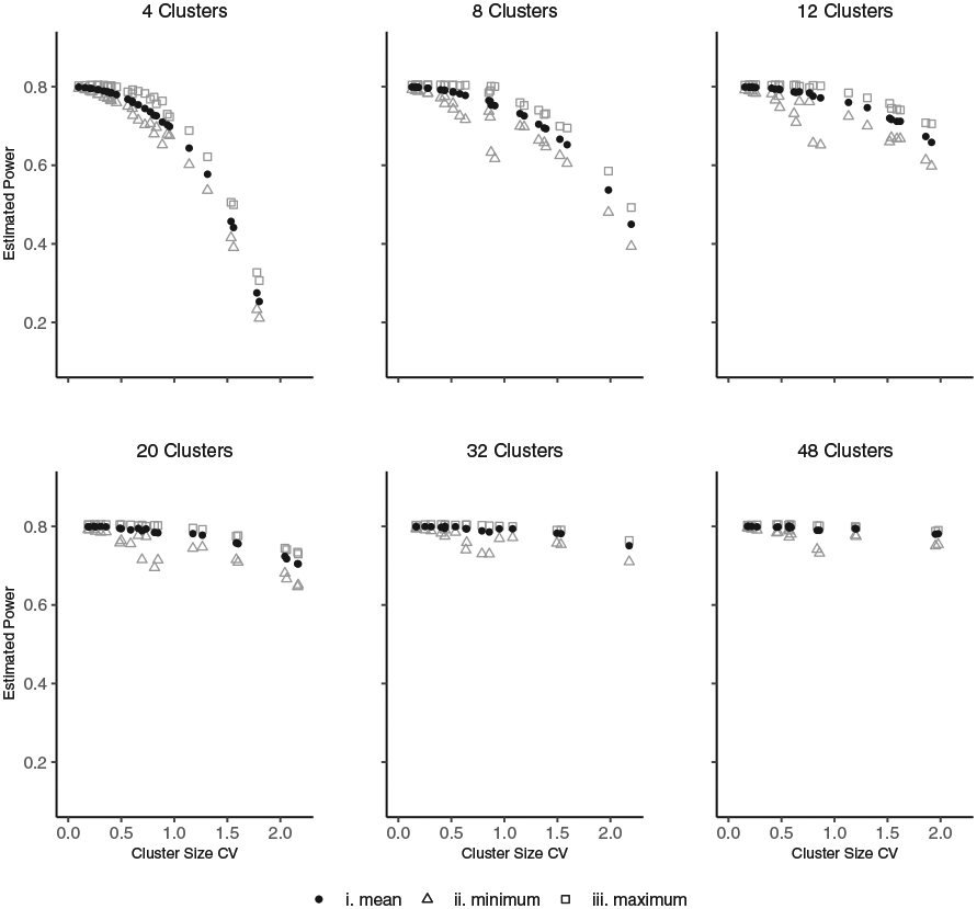
Effect of variable cluster sizes on estimated power for the exchangeable correlation structure. The effect size (log odds ratio between intervention and control, θ*) was fixed so that under equal cluster-period sizes of n = 30 there would be 80% power for a design with ρ = 0.05, T = 5, I = 4, 8, 12, 20, 32 and 48, q = 1, 2, 3, 5, 8 and 12, respectively. Cluster-period sizes were varied so that the arithmetic mean cluster-period size remained at $\overline{n}=30$ and the cluster size coefficient of variation (CV) ranged from 0 to 2. One thousand randomization sequences (M = 1000) were explored and the mean, minimum and maximum power estimated by Equations (11) and (12), respectively, are displayed

3 ∣. SIMULATION STUDY

We conducted a simulation study to explore the number of clusters necessary to implement the power calculation methods based on the logistic model with discrete time-effects fitted by the GEE approach in finite samples. We considered scenarios with equal cluster sizes along with the exchangeable, nested exchangeable, exponential decay and heterogeneous treatment correlation structures. We estimated power based on the model-based variance of the treatment effect estimate, assuming the correlation structure is correctly specified. To simulate study power and type I error, we fitted the GEE model under the true correlation structure along with the model-based variance. Additionally, we considered the sandwich variance of Liang and Zeger,³¹ as well as the bias-corrected sandwich variance of Mancl and DeRouen³² (MD), under adoption of the true correlation structure, the working exchangeable structure and the working independence structure in the analysis. Furthermore, we studied the influence of cluster size variation under the exchangeable correlation structure.

3.1 ∣. Data generating process

3.1.1 ∣. Equal cluster sizes

Binary outcome data under the logistic marginal model with discrete time-effects and correlation corresponding to the exchangeable (Equation 4), nested exchangeable (Equation 6), exponential decay (Equation 7) and heterogeneous treatment (Equation 8) structures were simulated using the method of Qaqish³⁶ for the 72 scenarios outlined in Web Tables 1 and 3. For comparison purposes, firstly the number of measurement time-periods was fixed at T = 5; the number of clusters (I) was equal to 4, 8, 12, 20, 32, and 48, so that the number of cluster randomized at each step (q) was 1, 2, 3, 5, 8, and 12, respectively. Secondly, the number of measurement time-periods was fixed at T = 7; the number of clusters (I) was equal to 6, 18, and 36, so that the number of cluster randomized at each step (q) was 1, 3, and 6, respectively. The data were simulated under no intervention effect to calculate the type I error, as well as varying intervention effects (log odds ratios, θ*) so the estimated power was 80% for each scenario based on the Wald test of the treatment effect using the variance expression in Equation (5) along with the relevant correlation structure. A gently decreasing discrete time-effect was assumed. For each of these 72 simulation scenarios, the data were generated 1000 times.

3.1.2 ∣. Unequal cluster sizes

For each design the cluster sizes, n_i for all time-periods j = 1, … , T, were chosen so that the cluster size CV was large at 1.8 (Web Table 5). One thousand (M = 1000) randomization sequences were randomly selected, and the intervention effect fixed so that the mean estimated power based on the variance formula in Equation (11) was 80%. The minimum and maximum power was approximated from the 1000 selected sequences using the variance formula in Equation (12). Binary outcome data under the logistic marginal model with discrete time-effects and exchangeable correlation structure was simulated using the method of Qaqish.³⁶ For each of the 12 scenarios in Web Table 5, datasets corresponding to each of the 1000 chosen randomization sequences were simulated 10 times to calculate the mean power via simulation (10 000 replicates in total). To calculate the minimum and maximum power via simulation, datasets corresponding to the randomization sequence that had the minimum and maximum estimated power were generated 1000 times, respectively.

3.2 ∣. Analysis method

GEE models were fitted to each simulated dataset as described in Prentice.³⁷ For each simulated dataset, a model adopting the true correlation structure was fitted. For the exchangeable, nested exchangeable and heterogeneous treatment structures, the geeglm function in the R package geepack was used to fit the model. The nested exchangeable and heterogeneous treatment structures were “userdefined” by the “zcor” option. We were not able to find standard software that can fit the exponential decay structure, and therefore implemented a Fisher scoring algorithm as outlined in Web Appendix D. In addition to the true correlation structure, both a model adopting a working exchangeable and independence structure were fitted using geeglm. The model-based, sandwich and MD variance estimates (Web Appendix D) were used to test the treatment effect, and the simulated power was calculated by the proportion of times the two-sided Wald test rejected the null of no treatment difference at the 5% level.

3.3 ∣. Results

Figure 3 displays the simulation results for equal cluster sizes based on T = 5 time-periods. When there are 20 or more clusters, all three variance estimates result in the correct power close to 80% and type I error close to 5% when the true correlation structure is adopted in the analysis. When there are 4 to 12 clusters, as expected; the model-based variance continues to perform well, the sandwich variance results in inflated type I error so the power achieved by this approach is not relevant, and the MD variance maintains type I error but results in power loss. For the working exchangeable structure, the type I error and power are maintained at their nominal levels when there are 20 or more clusters and the sandwich or MD variance are utilized. The model-based variance results in inflated type I error due to model misspecification. For the working independence structure, while type I error is maintained near the 5% level for the sandwich and MD variances for 20 or more clusters, there is substantial efficiency loss; for example, in the design with 48 clusters the simulated power is between 38% and 57%. As anticipated, for a working independence structure, the model-based variance produces results with large type I errors of over 30%. Web Tables 1 and 2 provide detailed results for the simulations with T = 5 time-periods including the mean estimated correlation parameters. Simulations with T = 7 time-periods gave similar results (Web Figure 4, Web Tables 3 and 4).

FIGURE 3.

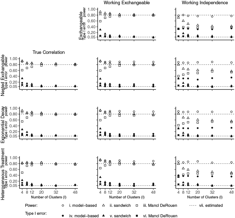
Simulated power and type I error with equal cluster sizes based on T = 5 time-periods. For each scenario, the effect size (log odds ratio between intervention and control, θ*) was fixed so that the estimated power was 80%. The power and type I error was simulated for the model-based, sandwich and Mancl-DeRouen variance by conducting 1000 replicates. The leftmost figure in each row displays the results from simulating the data under the indicated correlation structure and fitting the true correlation structure in the analysis. The middle figure displays the results from simulating the data under the true correlation structure and fitting a working exchangeable structure in the analysis. The rightmost figure displays the results from simulating the data under the true correlation structure and fitting a working independence structure in the analysis. For the first row, under an exchangeable correlation structure, fitting a working exchangeable correlation structure in the analysis corresponds to fitting the true correlation structure

The simulation results for variable cluster sizes are in Web Figure 5 and Web Table 5. For the true exchangeable correlation structure, the model-based variance performs well. The type I error for the sandwich variance reduces to 7.4% when there are 48 clusters. The MD variance maintains type I error below 5%, but results in efficiency loss. In fact, the efficiency loss from employing the MD variance is larger than that contributed by cluster size variation in this simulated scenario with large cluster size variation. For the working independence structure, we observe power loss for all three variances; particularly the MD variance.

R code to implement the power calculation methods and replicate the simulation study can be found at https://github.com/lindajaneharrison/SW-CRTs/releases/tag/v2.0.

4 ∣. ILLUSTRATIVE EXAMPLE

To demonstrate the methods outlined in the article to estimate the power of a cross-sectional SW-CRT with binary outcomes, we discuss a trial that evaluated whether a quality of care improvement intervention would result in better clinical outcomes among patients with acute coronary syndrome.^13,38 The study was designed to include 104 hospitals (the clusters), five time-periods (T = 5) consisting of a baseline time-period and four steps, where 26 clusters were randomly assigned to initiate the intervention at each step. To account for potential drop-out of hospitals, power calculation was based on 96 hospitals. The authors assumed an event rate of 8% for cardiovascular events, and stated the study would have 98% power at the two-sided 5% significance level to detect a relative risk reduction of 20% assuming an intercluster correlation of ρ = 0.1. In the trial design³⁸ and analysis,¹³ the authors planned and implemented a logistic GEE model, and based the primary analysis on an odds ratio comparing the intervention to control adjusting for discrete time-effects. If the study had assumed a binary outcome with an 8% probability of an event under control, and a 20% reduction under intervention, we would calculate the power to detect a difference of 8% vs 6.4% implying a log odds ratio of −0.24.

We now illustrate the power calculation methods outlined in this article for assessing a prevalence difference or log odds ratio, with and without time-effect adjustment. Under the linear model with no time-effect (Web Appendix A), the study would have 98.2% power (Table 3). As expected, using the logistic model with no time-effect (Web Appendix A) resulted in lower power of 97.8%; but the reduction was negligible. Now, adding adjustment for time, based on the linear model in Equation (2) the power reduces to 71.0%, which represents a large reduction due to discrete time-effect adjustment. If more accurately, a logistic GEE is assumed with time-effect adjustment (Equation 4) and there is a time trend such that the probability of an event decreases between the first and second time-period so β₁ = logit(0.08) = −2.44 and β_j = logit(0.08) − 0.15 = −2.59 for j = 2, … , T, we calculate the study power to be 64.4%.

TABLE 3.

Illustrative example scenarios

8% vs 6.4%, log odds ratio θ* = −0.24, $\overline{\mathit{n}}=40$
Correlation Structure	Model	Equations	${\beta }_1^{\ast },{\beta }_2^{\ast },{\beta }_3^{\ast },{\beta }_4^{\ast },{\beta }_5^{\ast }$	CV	Power (%)
Exch. ρ = 0.1	Linear, no time	a	Not required		98.2
Exch. ρ = 0.1	Logistic, no time	a	Not required		97.8
Exch. ρ = 0.1	Linear, time adj.	2, 3	Not required		71.0
Exch. ρ = 0.1	Logistic, time adj.	4, 5	−2.44, −2.59, −2.59, −2.59, −2.59		64.4
Nested exch. ρ1 = 0.1, ρ2 = 0.01	Logistic, time adj.	5, 6	−2.44, −2.59, −2.59, −2.59, −2.59		24.0
Exp. decay τ = 0.1, ρ = 0.56	Logistic, time adj.	5, 7	−2.44, −2.59, −2.59, −2.59, −2.59		26.5
Het. ρ1 = 0.1, ρ2 = 0.02, ρ3 = 0.08	Logistic, time adj.	5, 8	−2.44, −2.59, −2.59, −2.59, −2.59		24.8
Exch. ρ = 0.1	Logistic, time adj.	11, 12	−2.44, −2.59, −2.59, −2.59, −2.59	0.32	Mean: 64.3 Min: 63.4, max: 64.8
Exch. ρ = 0.1	Logistic, time adj.	11, 12	−2.44, −2.59, −2.59, −2.59, −2.59	1.04	Mean: 64.0 min: 61.8, max: 64.9

Abbreviations: adj., adjustment; CV, cluster size coefficient of variation; exch., exchangeable; exp., exponential; het., heterogeneous treatment.

^aEquations in Web Appendix A.

Next, we consider the impact of more complex correlation structures. An intercluster correlation of ρ = 0.1 was assumed in the power calculation based on a previous CRT, however the estimated ρ in the analysis was 0.01. Among other reasons, one explanation could be that the correlation reduced as the time between measurements increased, or that the correlation reduced when clusters initiated the intervention. We calculated a power of 24.0% for the nested exchangeable structure with a within-period correlation of ρ₁ = 0.1 and an interperiod correlation of ρ₂ = 0.01. For the exponential decay structure, we assumed τ = 0.1 and ρ = 0.56, so the correlation between outcomes in the same cluster and time-period was 0.1, and this correlation decayed over time such that the correlation between outcomes in the same cluster four time-periods apart was 0.1 × 0.56⁴ = 0.01. The power in this case was 26.5%. Finally, assuming a heterogeneous treatment structure with correlation for two individuals on control of ρ₁ = 0.1, two individuals on intervention of ρ₃ = 0.08, and for one individual on control and one on intervention of ρ₂ = 0.02, the study power would be 24.8%.

Lastly, to gain some insight into the impact of varying cluster sizes, we assumed the exchangeable correlation structure with ρ = 0.1 and mapped hospital size information¹³ to cluster sizes to produce moderate (CV = 0.32) and large (CV = 1.04) cluster size variation. Based on 1000 randomization sequences, the mean power was estimated to be 64.3% (min. 63.4, max. 64.8) and 64.0% (min. 61.8, max. 64.9) for moderate and large variation, respectively (Table 3). Since there are a large number of clusters, the power reduction due to cluster size variation is small.

5 ∣. DISCUSSION

In the rapidly evolving field of SW-CRTs, binary outcome measures commonly arise.^4-6 Power calculation methods have focused on a linear model with normal approximation for binary outcomes.^16,17 In this article, we illustrate that accounting for a logistic marginal model at the study planning stage, when this is the planned analysis method, tends to result in lower estimated power than when a linear model is incorrectly assumed. The reduction in power is larger when there are a smaller number of individuals at each time-period and fewer time-periods. When the outcome is rare or very common, a higher intercluster correlation will result in a larger reduction in power; however when the outcome has close to a 50% prevalence, the intercluster correlation has little impact on the reduction in power. Importantly, if the outcome prevalence decreases toward 0% or increases toward 100% (ie, moves away from 50% prevalence) during the study, the power to detect a fixed log odds ratio can decrease substantially. Therefore, we recommend performing power calculation based on the logistic marginal model taking into account an anticipated time trend when this will be the analysis method. A power sensitivity analysis that specifies a plausible time trend with an outcome prevalence moving away from 50% over the course of the study would be a conservative approach. Li et al²⁰ proposed methods for cohort SW-CRTs under the nested exchangeable correlation structure. In this article, we provide power calculation techniques for binary outcomes under several correlation structures for cross-sectional SW-CRTs.

As previously noted for the linear²⁴ and logistic²⁹ model, it is important in the trial planning stage to account for the fact a SW-CRT should include time adjustment. This adjustment, using discrete time-effects, will result in lower power, and is therefore an important consideration. Similarly, it is worth exploring more complex correlation structures when planning a SW-CRT. As highlighted by Hooper et al,²⁵ Kasza et al²⁷ and others, in cross-sectional SW-CRTs the correlation of outcome measures within the same cluster is likely to reduce as the time period between measurements increases. In this circumstance for the logistic model the power would be lower using the nested exchangeable or exponential decay correlation structure than the exchangeable structure.

Since the treatment status variable is changing within a cluster in the SW-CRT design, when a GEE approach is used for the trial analysis, adopting a working independence correlation structure along with a sandwich variance will result in efficiency loss.³⁹ This finding has been observed in simulation studies of SW-CRTs with continuous outcomes,³³ and is confirmed here for binary outcomes. Interestingly, adopting a working exchangeable correlation structure along with a sandwich variance resulted in similar power to an analysis utilizing the true more complex correlation structure when there were 20 or more clusters. Therefore, it appears less important to fit the correct correlation structure in the analysis phase when implementing a GEE approach because adopting an exchangeable correlation structure is satisfactory.

When there were fewer than 20 clusters, we observed small sample downward bias of the sandwich variance.³¹ Therefore, to maintain type I error at the nominal level, we implemented the bias-corrected sandwich variance of Mancl and DeRouen.³² This bias-corrected variance performed well and maintained the type I error close to 5% when there were 8 or more clusters. It did result in a modest reduction of power, with a smaller reduction as the number of clusters increased. Other finite sample sandwich variance corrections, such as the Kauerman and Carroll⁴⁰ and Fay and Grubard⁴¹ corrections, have been explored in the context of SW-CRTs with binary outcomes;^20,30 we choose to implement the Mancl and DeRouen correction as it appeared to have the best trade-off between type I error control and maintenance of power in previous literature.²⁰ Another adaptation could employ the matrix-adjusted GEEs of Preisser and Qaqish,⁴² since when there are a small number of clusters this additional adjustment should result in less finite sample bias in correlation estimation. We choose to primarily use a standard R package (geepack) that does not employ matrix adjustment, and the approach resulted in adequate correlation parameter estimates.

We implemented a Fisher scoring algorithm to incorporate the exponential decay correlation structure of Kasza et al.²⁷ This structure allows the correlation between outcomes in the same cluster to decay as the number of time-periods between them increases. It is most appropriate if all individuals in the same period are measured at approximately the same time. Under a LME modeling framework, Grantham et al⁴³ extended this idea to accommodate continuous enrollment allowing the correlation decay to depend on the distance between the actual measurement times. Further extension to a model with a logit link should be possible.

In general, the estimated impact of unequal cluster sizes on study power is modest, unless there are a small number of clusters and extensive cluster size variation. Therefore, in scenarios where there are enough clusters to employ the sandwich variance of Liang and Zeger,³¹ unequal cluster sizes do not appear to impact power substantially for realistic levels of cluster size heterogeneity. In scenarios with fewer clusters it is advisable to implement a bias-corrected sandwich variance, such as that of Mancl and DeRouen,³² to maintain type I error as well as robustness to correlation misspecification. In this case, the power loss from the conservativeness of this bias-corrected variance is larger than that from cluster size variation. Lastly, we choose to adopt a marginal model in our exploration of power for binary outcomes. This allows the interpretation of the intervention effect to remain the same regardless of the correlation structure. An alternative would be to consider GLMMs where the intervention effect is conditional upon the random-effects. Using simulation techniques, Barker et al²⁹ compared the analysis of a SW-CRT with a binary outcome and a logit link function under a GEE with a working exchangeable correlation structure to a GLMM with a random-intercept. Additionally, Baio et al²¹ described a simulation approach to estimate power with equal cluster sizes under a GLMM framework for certain random-intercept models. Extending these simulation approaches to estimate power for more complex random-effect structures may not be straightforward since for binary outcomes with a logit link function it is likely fitting procedures will be computationally intensive due to the need to integrate out the random-effects. Future research could explore power estimation under a logit GLMM via approximation.^10,11,44

DATA AVAILABILITY STATEMENT

Data sharing is not applicable to this article as no new data were created or analyzed in this study.

REFERENCES

- 1.Brown CA, Lilford RJ. The stepped wedge trial design: a systematic review. BMC Med Res Methodol. 2006;6(1):54. [DOI] [PMC free article] [PubMed] [Google Scholar]
- 2.Beard E, Lewis JJ, Copas A, et al. Stepped wedge randomised controlled trials: systematic review of studies published between 2010 and 2014. Trials. 2015;16(1):353. [DOI] [PMC free article] [PubMed] [Google Scholar]
- 3.Hemming K, Haines TP, Chilton PJ, Girling AJ, Lilford RJ. The stepped wedge cluster randomised trial: rationale, design, analysis, and reporting. BMJ. 2015;350:h391. 10.1136/bmj.h391 [DOI] [PubMed] [Google Scholar]
- 4.Martin J, Taljaard M, Girling A, Hemming K. Systematic review finds major deficiencies in sample size methodology and reporting for stepped-wedge cluster randomised trials. BMJ Open. 2016;6(2):e010166. 10.1136/bmjopen-2015-010166 [DOI] [PMC free article] [PubMed] [Google Scholar]
- 5.Barker D, McElduff P, D’Este C, Campbell MJ. Stepped wedge cluster randomised trials: a review of the statistical methodology used and available. BMC Med Res Methodol. 2016;16:69. 10.1186/s12874-016-0176-5 [DOI] [PMC free article] [PubMed] [Google Scholar]
- 6.Davey C, Hargreaves J, Thompson JA, et al. Analysis and reporting of stepped wedge randomised controlled trials: synthesis and critical appraisal of published studies, 2010 to 2014. Trials. 2015;16:358. 10.1186/s13063-015-0838-3 [DOI] [PMC free article] [PubMed] [Google Scholar]
- 7.Shih WJ. Sample size and power calculations for periodontal and other studies with clustered samples using the method of generalized estimating equations. BiomJ. 1997;39(8):899–908. [Google Scholar]
- 8.Pan W Sample size and power calculations with correlated binary data. Control Clin Trials. 2001;22(3):211–227. [DOI] [PubMed] [Google Scholar]
- 9.Liu A, Shih W, Gehan E. Sample size and power determination for clustered repeated measurements. Stat Med. 2002;21(12):1787–1801. [DOI] [PubMed] [Google Scholar]
- 10.Moerbeek M, Van Breukelen GJ, Berger MP. Optimal experimental designs for multilevel logistic models. J Royal Stat Soc Ser D (Stat). 2001;50(1):17–30. [Google Scholar]
- 11.Candel MJ, Van Breukelen GJ. Sample size adjustments for varying cluster sizes in cluster randomized trials with binary outcomes analyzed with second-order PQL mixed logistic regression. Stat Med. 2010;29(14):1488–1501. [DOI] [PubMed] [Google Scholar]
- 12.Rutterford C, Copas A, Eldridge S. Methods for sample size determination in cluster randomized trials. Int J Epidemiol. 2015;44(3):1051–1067. 10.1093/ije/dyv113 [DOI] [PMC free article] [PubMed] [Google Scholar]
- 13.Wu Y, Li S, Patel A, et al. Effect of a quality of care improvement initiative in patients with acute coronary syndrome in resource-constrained hospitals in china: a randomized clinical trial. JAMA Cardiol. 2019;4(5):418–427. 10.1001/jamacardio.2019.0897 [DOI] [PMC free article] [PubMed] [Google Scholar]
- 14.Hussey MA, Hughes JP. Design and analysis of stepped wedge cluster randomized trials. Contemp Clin Trials. 2007;28(2):182–191. 10.1016/j.cct.2006.05.007 [DOI] [PubMed] [Google Scholar]
- 15.Hemming K, Girling A. A menu-driven facility for power and detectable-difference calculations in stepped-wedge cluster-randomized trials. Stata J. 2014;14(2):363–380. [Google Scholar]
- 16.Hemming K, Kasza J, Hooper R, Forbes A, Taljaard M. A tutorial on sample size calculation for multiple-period cluster randomized parallel, cross-over and stepped-wedge trials using the shiny CRT calculator. Int J Epidemiol. 2020;49(3):979–995. 10.1093/ije/dyz237 [DOI] [PMC free article] [PubMed] [Google Scholar]
- 17.Voldal EC, Hakhu NR, Xia F, Heagerty PJ, Hughes JP. swCRTdesign: an R package for stepped wedge trial design and analysis. Comput Methods Prog Biomed. 2020;196:105514. [DOI] [PMC free article] [PubMed] [Google Scholar]
- 18.Zhou X, Liao X, Kunz LM, Normand SLT, Wang M, Spiegelman D. A maximum likelihood approach to power calculations for stepped wedge designs of binary outcomes. Biostatistics. 2020;21(1):102–121. [DOI] [PMC free article] [PubMed] [Google Scholar]
- 19.Li F, Hughes JP, Hemming K, Taljaard M, Melnick ER, Heagerty PJ. Mixed-effects models for the design and analysis of stepped wedge cluster randomized trials: an overview. Stat Methods Med Res. 2021;30(2):612–639. 10.1177/0962280220932962 [DOI] [PMC free article] [PubMed] [Google Scholar]
- 20.Li F, Turner EL, Preisser JS. Sample size determination for GEE analyses of stepped wedge cluster randomized trials. Biometrics. 2018;74:1450–1458. 10.1111/biom.12918 [DOI] [PMC free article] [PubMed] [Google Scholar]
- 21.Baio G, Copas A, Ambler G, Hargreaves J, Beard E, Omar RZ. Sample size calculation for a stepped wedge trial. Trials. 2015;16:354. 10.1186/s13063-015-0840-9 [DOI] [PMC free article] [PubMed] [Google Scholar]
- 22.Martin JT, Hemming K, Girling A. The impact of varying cluster size in cross-sectional stepped-wedge cluster randomised trials. BMC Med Res Methodol. 2019;19(1):123. 10.1186/s12874-019-0760-6 [DOI] [PMC free article] [PubMed] [Google Scholar]
- 23.Harrison LJ, Chen T, Wang R. Power calculation for cross-sectional stepped wedge cluster randomized trials with variable cluster sizes. Biometrics. 2019;76:951–962. 10.1111/biom.13164 [DOI] [PMC free article] [PubMed] [Google Scholar]
- 24.Zhou X, Liao X, Spiegelman D. “Cross-sectional” stepped wedge designs always reduce the required sample size when there is no time effect. J Clin Epidemiol. 2017;83:108–109. 10.1016/j.jclinepi.2016.12.011 [DOI] [PMC free article] [PubMed] [Google Scholar]
- 25.Hooper R, Teerenstra S, de Hoop E, Eldridge S. Sample size calculation for stepped wedge and other longitudinal cluster randomised trials. Stat Med. 2016;35(26):4718–4728. 10.1002/sim.7028 [DOI] [PubMed] [Google Scholar]
- 26.Girling AJ, Hemming K. Statistical efficiency and optimal design for stepped cluster studies under linear mixed effects models. Stat Med. 2016;35(13):2149–2166. [DOI] [PMC free article] [PubMed] [Google Scholar]
- 27.Kasza J, Hemming K, Hooper R, Matthews J, Forbes AB. Impact of non-uniform correlation structure on sample size and power in multiple-period cluster randomised trials. Stat Methods Med Res. 2019;28(3):703–716. 10.1177/0962280217734981 [DOI] [PubMed] [Google Scholar]
- 28.Hughes JP, Granston TS, Heagerty PJ. Current issues in the design and analysis of stepped wedge trials. Contemp Clin Trials. 2015;45(Pt A):55–60. 10.1016/j.cct.2015.07.006 [DOI] [PMC free article] [PubMed] [Google Scholar]
- 29.Barker D, D’Este C, Campbell MJ, McElduff P. Minimum number of clusters and comparison of analysis methods for cross sectional stepped wedge cluster randomised trials with binary outcomes: a simulation study. Trials. 2017;18(1):1–11. [DOI] [PMC free article] [PubMed] [Google Scholar]
- 30.Ford WP, Westgate PM. Maintaining the validity of inference in small-sample stepped wedge cluster randomized trials with binary outcomes when using generalized estimating equations. Stat Med. 2020;39(21):2779–2792. [DOI] [PubMed] [Google Scholar]
- 31.Liang KY, Zeger SL. Longitudinal data analysis using generalized linear models. Biometrika. 1986;73(1):13–22. [Google Scholar]
- 32.Mancl LA, DeRouen TA. A covariance estimator for GEE with improved small-sample properties. Biometrics. 2001;57(1):126–134. [DOI] [PubMed] [Google Scholar]
- 33.Ren Y, Hughes JP, Heagerty PJ. A simulation study of statistical approaches to data analysis in the stepped wedge design. Stat Biosci. 2020;12:319–415. [DOI] [PMC free article] [PubMed] [Google Scholar]
- 34.Hemming K, Girling A. A menu-driven facility for power and detectable-difference calculations in stepped-wedge cluster-randomized trials. Erratum Stata J. 2016;16(1):243–243. [Google Scholar]
- 35.Kasza J, Bowden R, Forbes AB. Information content of stepped wedge designs with unequal cluster-period sizes in linear mixed models: informing incomplete designs. Stat Med. 2021;40(7):1736–1751. [DOI] [PubMed] [Google Scholar]
- 36.Qaqish BF. A family of multivariate binary distributions for simulating correlated binary variables with specified marginal means and correlations. Biometrika. 2003;90(2):455–463. [Google Scholar]
- 37.Prentice RL. Correlated binary regression with covariates specific to each binary observation. Biometrics. 1988;44(4):1033–1048. [PubMed] [Google Scholar]
- 38.Li S, Wu Y, Du X, et al. Rational and design of a stepped-wedge cluster randomized trial evaluating quality improvement initiative for reducing cardiovascular events among patients with acute coronary syndromes in resource-constrained hospitals in China. Am Heart J. 2015;169(3):349–355. 10.1016/j.ahj.2014.12.005 [DOI] [PubMed] [Google Scholar]
- 39.Mancl LA, Leroux BG. Efficiency of regression estimates for clustered data. Biometrics. 1996;52(2):500–511. [PubMed] [Google Scholar]
- 40.Kauermann G, Carroll RJ. A note on the efficiency of sandwich covariance matrix estimation. J Am Stat Assoc. 2001;96(456):1387–1396. [Google Scholar]
- 41.Fay MP, Graubard BI. Small-sample adjustments for Wald-type tests using sandwich estimators. Biometrics. 2001;57(4):1198–1206. [DOI] [PubMed] [Google Scholar]
- 42.Preisser JS, Lu B, Qaqish BF. Finite sample adjustments in estimating equations and covariance estimators for intracluster correlations. Stat Med. 2008;27(27):5764–5785. [DOI] [PubMed] [Google Scholar]
- 43.Grantham KL, Kasza J, Heritier S, Hemming K, Forbes AB. Accounting for a decaying correlation structure in cluster randomized trials with continuous recruitment. Stat Med. 2019;38(11):1918–1934. [DOI] [PubMed] [Google Scholar]
- 44.Xia F, Hughes JP, Voldal EC, Heagerty PJ. Stepped wedge designs: power and sample size calculation with discrete outcomes. Paper presented at: Proceedings of the 3rd International Conference on Stepped Wedge Trial Design; York UK (virtual) 2021. [DOI] [PMC free article] [PubMed] [Google Scholar]
Associated Data
This section collects any data citations, data availability statements, or supplementary materials included in this article.
Supplementary Materials