A Primer on EEG Spectrograms

Summary:

As continuous brain monitoring becomes a routine part of clinical care, continuous EEG has allowed better detection and characterization of nonconvulsive seizures, and patterns along the ictal–interictal continuum in critically ill patients. However, this increased workload has led many to turn to quantitative EEG whose central tool is the “spectrogram.” Although in relatively wide use, many clinicians lack a detailed understanding of how spectrograms relate to the underlying “raw” EEG signal. This article provides an approachable set of first principles to help clinicians understand how spectrograms encode information about the raw EEG and how to interpret spectrograms to efficiently infer underlying EEG patterns.

Continuous brain monitoring is becoming a routine part of clinical care. Continuous EEG has translated into better detection and characterization of nonconvulsive seizures and patterns along the ictal–interictal continuum in critically ill patients but at the cost of greatly increased clinical work.¹ This situation has led many medical centers to adopt quantitative EEG to improve efficiency.² The central tool in quantitative EEG, the “spectrogram,” also known as color spectral array or color density spectral array, is standard in most quantitative EEG software. The spectrogram is typically displayed as a three-way plot of time on the x axis, frequency on the y axis, and power as color.³ Although spectrograms are now widely used, most clinicians lack a detailed understanding of how spectrograms relate to features of the underlying “raw” EEG signal. This article provides an approachable set of first principles to help clinicians understand how spectrograms encode information about the raw EEG and how to interpret spectrograms to efficiently infer underlying EEG patterns.

OSCILLATING BACKGROUNDS: REGULAR VERSUS CHANGING SIGNALS

The surface EEG is a representation of postsynaptic potentials generated in the cerebral cortex.⁴ This signal is sampled at discrete time points (i.e., with a certain sampling frequency), and the voltage samples are interpolated to generate a signal that is displayed on a computer screen (Fig. 1).

FIG. 1.

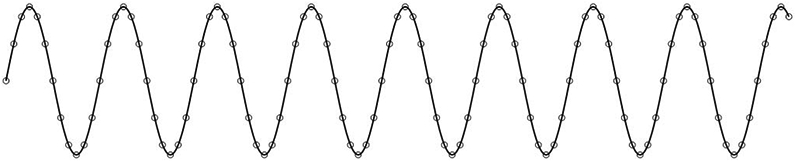
Interpolation of data sampled at discrete time points to generate a signal.

Over short periods (e.g., < 1 second), EEG signals often appear as oscillating waves. An oscillating signal is a regularly repeating pattern with a few fundamental properties of interest to the clinician (Fig. 2). First, the frequency f is how often the wave repeats itself over time. Frequency is measured in Hertz (Hz), the number of oscillations per second. Second, the phase θ is the timing of the wave relative to where it is along its cycle. Phase shifting a perfectly regular oscillatory signal backward or forward in time by one complete cycle brings the wave back to its original timing. Phase is measured in degrees (°) or radians (units of π). Next, there is amplitude A, which is the average distance between peaks to troughs, measured in microvolts (μV). Finally, there is power P, the square of the amplitude A². Power is often displayed on a logarithmic scale, in decibels dB.

FIG. 2.

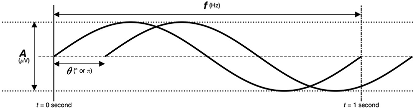
Fundamental wave properties.

Like any signal, an EEG signal always has an associated “spectrum,” meaning that it is always possible to decompose a signal into a series of sine waves and cosine waves. It is also possible to reconstruct the EEG signal from the same spectrum of sine and cosine waves. The spectrum of sine and cosine waves is also called the “frequency domain” representation of the signal. Otherwise, the signal itself is in the “time domain.” The mathematical formula that allows us to move back and forth between time and frequency domains is the “Fourier transformation” (Fig. 3).

FIG. 3.

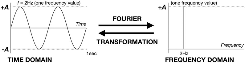
Schematic of Fourier transformation.

Some oscillating signals have very simple spectra, whereas others demonstrate complicated spectra. Regular oscillations can be made up of contributions from a relatively small number of sine and cosine waves. For example, a pure sine wave includes only one frequency, which means that its spectrum has non-zero amplitude for just this single frequency f. In contrast, signals that are irregular and changing are more complicated, and, are composed of a mixture of oscillations with a broader spectrum and contributions from a larger number of sine and cosine waves. These EEG signals can be constructed (or broken down into) a linear weighted average of sine and cosine waves (Fig. 4).

FIG. 4.

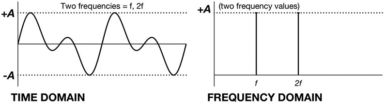
An example of mixing oscillations in the time and frequency domains.

The best approximation to a simple sinusoidal wave in real-life EEG is the posterior dominant rhythm (PDR) in the alpha frequency range (f = 8–13 Hz). The PDR is a normal waking background rhythm seen predominantly over the occipital regions during relaxed periods with the eyes closed. A 10-second EEG segment of PDR is shown in Fig. 5A.⁵ Its power spectrum is shown in Fig. 5B on a logarithmic scale in decibels dB (derived from power P).⁵ A prominent peak is present at approximately 9.5 Hz.

FIG. 5.

The EEG and power spectra of the posterior dominant rhythm (A and B) and a non-regular signal (C and D).

Unlike the PDR, most EEG background signals are composed of a broad mixture of oscillations rather than from waves limited to a particular narrow band of frequencies. An example of such a motley crew of frequencies is shown in Fig. 5C.⁵ This signal shows a mixture of delta, theta, and faster oscillations. Accordingly, the spectrum in Fig. 5D shows the highest power in the delta (0–4 Hz) range.⁵ This power persists but decreases in an approximately linear fashion across the 0 to 20 Hz range.

TRANSIENT EVENTS: FOREGROUND SIGNALS WITH SHAPE

Even more “complex” than irregular signals are nonoscillating transient events with a distinct shape, such as an epileptic spike. Although the EEG background may be thought of as a relatively simple mixture of ongoing oscillations, transients in the EEG can be thought of as “foreground” events that burst through and stand out from the background. Examples of EEG transients include isolated interictal epileptiform discharges (such as sharp waves and spikes), periodic epileptiform discharges, and seizures. Like oscillating signals, transient events can also be decomposed into a series of oscillations. However, constructing sharp turns in a signal to render a sharper waveform requires more oscillations, which translates into a broader spectrum.

Let us first construct a spike–wave complex (i.e., a single, isolated, interictal epileptiform discharge) using component oscillations (Fig. 6).⁵ Our approximation becomes more accurate as we include a larger number of components. The top row (Fig. 6A) shows a spike and wave discharge (black) together with the approximations (red) constructed using 2 (left-most column) to 15 (right-most column) component sinusoids.⁵ Each sinusoid is depicted in the second row (Fig. 6B) and the amplitude spectrum (amplitude of each component sinusoid as a function of frequency) is shown in the third row (Fig. 6C).⁵

FIG. 6.

Constructing a spike–wave complex (A) by adding more sinusoids (B) with corresponding power spectra (C).

Similarly, more component oscillations are required to construct narrower transients; specifically, for constructive and destructive interference to render sharper “turns” in the signal (Fig. 7).⁵ It follows that a signal’s power spectrum is not only a function of the frequencies of the background oscillations but also a function of the signal’s shape, with sharp or spiky signal features producing higher frequency components in the spectrum.

FIG. 7.

Constructing a spikier wave (A) by adding more sinusoids (B) with corresponding power spectra (C).

When interictal epileptiform discharges become repetitive (i.e., as periodic discharges), describing them in terms of oscillations is even more complicated. Rather than describing the isolated events in terms of a spectrum as a function of amplitude (as we have been doing), it is more useful to describe the spectrum as a function of time, that is, as a spectrogram.

Simulated periodic discharges at different frequencies are shown in Fig. 8 (A: 1 Hz, B: 3 Hz, C: 5 Hz).⁵ The interdischarge intervals of these simulated periodic discharges are only approximately equal to mirror the fact that real-life periodic discharges do not occur at exactly regular intervals. Considering the resultant spectrograms, first there is high power in the frequency at which the pattern is repeating, sometimes called the “fundamental frequency” f₀. In addition to f₀, there are also frequency bands at multiples of these frequencies because when a pattern repeats with frequency f₀, it also repeats at multiples of that frequency (e.g., 2f₀, 3f₀, etc.) called harmonics (or harmonic frequencies). Finally, the spikiness of the periodically repeating element also adds to the power at high frequencies because high-frequency sinusoids are needed to render rapid changes in the signal as sharp turns.

FIG. 8.

Simulated periodic discharges at 1 (A), 3 (B), and 5 Hz (C) with corresponding spectrograms.

OSCILLATIONS, TRANSIENTS, AND EVENTS: SPECTROGRAM SEIZURES

A seizure is a transient EEG event that evolves. In other words, a seizure is all of the above that we have been considering: oscillations, transients, and an event with a beginning and end. During a seizure, the frequency, morphology, and amplitude of the EEG signal may all change over time. In Fig. 9A, an idealized (simulated) seizure at one pure frequency increases in frequency and amplitude over time.⁵ Its spectrogram in Fig. 9B shows an upward-sloping band whose color changes from green to red as the signal power increases.⁵

FIG. 9.

A simulated seizure (A) with corresponding spectrogram (B). A real seizure (C) with corresponding spectrograms (D). Power spectra from selected times in C and D (E).

Real seizures typically possess a variety of frequencies and morphologies with different component oscillations as shown in Fig. 9C.⁵ This seizure begins around t = 0.25 minutes, increases in frequency and amplitude in crescendo fashion, until reaching peak intensity around t = 1 minute, and then decrescendos before ending around t = 2 minutes. These dynamics are shown in the time-aligned spectrogram in Fig. 9D.⁵ The corresponding power spectra of selected vertical blue rectangles (“time slices”) between Figs. 9C and 9D are shown in Fig. 9E.⁵

It should be noted that the spectrogram within these time slices in Fig. 9D shows the same information as in Fig. 9E (i.e., power spectra) except that the x axis of Fig. 9E (i.e., frequency) is plotted as the spectrogram y axis of Fig. 9D, and the y axis of Fig. 9E (i.e., power in decibels) is plotted as spectrogram color of Fig. 9D.⁵

With the exception of electrodecremental events, seizures on the spectrogram are represented by high power and high frequencies, which can represent spiky ictal discharges. Very high frequencies represent oscillatory activities, such as ictal fast activity (i.e., “beta buzz”). These characteristics can help alert the clinician to the presence of seizures and status epilepticus on the spectrogram.

SPECTROGRAM LIMITATIONS: DETAIL VERSUS NOISE

In real-world intensive care unit monitoring, the EEG signal is never perfectly regular. Rather, the EEG signal is best regarded as random: it contains an underlying signal of interest plus unwanted noise. Given this randomness, the EEG power spectrum and its spectrogram need to be estimated. To accurately estimate EEG power at a particular frequency, we need to perform some type of averaging or “smoothing” over a specified “time window” of data T to generate a spectral “estimate” from the finite-length signal residing inside our window. Window size is usually chosen based on either the maximum window length over which the signal can be considered stable or based on the desired level of temporal (time) resolution.

In Fig. 10A, we show a 15-second sample of a simulated random signal generated by a model whose true power spectrum is known, which is represented by a red curve against the estimated power spectra (in blue) of Figs. 10B-10E.⁵ The true spectrum in red has two peaks at approximately 11 and 14 Hz. Let us now choose a set window size T = 15 seconds. One way to estimate the power spectrum is to calculate the discrete Fourier transformation, using an algorithm known as the “fast Fourier transform”, and then take the squared amplitude of the result as an estimate of the power spectrum. The result is shown as the blue line in Fig. 10B.⁵ The power spectrum appears very noisy because it is estimated using only a single sample. Such estimates are called “periodograms”.

FIG. 10.

A simulated random signal (A) with known power spectrum (red line in B–E) and estimates of power spectrum (blue line in B–E).

Although we could obtain better estimates of the true spectrum by averaging multiple periodogram samples in a controlled experimental setting, we cannot hold a patient’s state constant to obtain repeated samples. Another method is required to reduce the variance of the spectral estimate, such as smoothing the spectrogram. Figures 10C-10E show progressively more smoothing of the original estimated signal in blue.⁵ However, smoothing blurs together fine spectral details, and beyond a certain point, the spectral peaks of the actual signal (red line) become indistinguishable in the estimated signal (blue line) of the most aggressive example of smoothing from Fig. 10E.⁵

The spectral resolution is defined as the minimum distinguishable difference between two peaks of an estimated power spectrum. In our examples, the approximate respective spectral resolutions are <1 Hz (Fig. 10C), 2 Hz (Fig. 10D), and 5 Hz (Fig. 10E).⁵ The optimal trade-off between smoothing to decrease noise (i.e., variance reduction) and enhancing detail (i.e., spectral resolution) seems to be achieved in Fig. 10D.⁵ This “detail versus noise” trade-off is technically known as the “bias-variance trade-off.” With more spectral resolution comes more noise, but with less noise comes less spectral resolution.

As another example, Fig. 11 shows a real PDR EEG signal instead of a simulated one and its resultant spectrogram alongside its power spectrum.⁵ From a 4-second segment of raw PDR EEG signal, we have estimated three 5-minute spectrogram samples of the same EEG signal with different spectral resolutions W. In the “high-resolution” (W = 0.25 Hz) spectrogram estimate, much detail appears to be noise. In the “low-resolution” (W = 4 Hz) spectrogram estimate, the smoothing appears excessive, which blurs out detail and distorts the underlying spectrum, introducing bias in the process of “reducing variance.” In contrast, the “medium-resolution” (W = 1.5 Hz) spectrogram estimate appears to strike an appropriate trade-off between detail and noise as in Fig. 10D. The optimal degree of spectral smoothing depends on the intrinsic smoothness of the underlying process that generates the signal and will vary depending on the application. A spectral resolution of approximately 1 Hz is typically sufficient for spectral smoothing and high-quality spectral estimates in clinical ICU EEG monitoring.

FIG. 11.

A real sample of posterior dominant rhythm with spectrograms of differing spectral resolutions.

SPECTROGRAM LIMITATIONS: TEMPORAL VERSUS SPECTRAL RESOLUTION

Up to this point, we have only considered trade-offs when the window size T remains constant. Another trade-off in computing spectrograms occurs when window size T changes. Specifically, a shorter window size of time T allows finer temporal detail (i.e., temporal resolution) but at the expense of more noise. To illustrate this, Fig. 12A shows a 20-second EEG segment with many epileptic spikes.⁵ In Figs. 12B, 12C, and 12D, the resultant 20-second spectrograms are calculated with sliding windows of width T = 4, 2, and 1 second, respectively.⁵ The spectrogram computed with the widest temporal window (Fig. 12B; T = 4 seconds) is smoothest but also has the poorest temporal resolution with none of the spikes distinctly visible.⁵ In contrast, spikes are clearly visible in the spectrogram with the shortest temporal window (Fig. 12D; T = 1 second), but this is the noisiest of all spectrograms.⁵

FIG. 12.

A simulated train of epileptic spikes (A) with spectrograms of progressively smaller window sizes T (B–D).

In addition to more noise, if we decrease window size T to increase temporal resolution, then we also decrease the spectral resolution. This trade-off is because of the consequences of the “Nyquist theorem,” which states that the maximum spectral resolution (equal to approximately twice the sampling rate) is directly proportional to the length of the signal segment T. Assuming a constant sampling rate, shrinking window size T reduces the number of high-frequency sinusoids available to represent the signal, which degrades our ability to distinguish fine detail in the frequency domain to decrease spectral resolution.

This “temporal-spectral resolution trade-off” is mathematically like the Heisenberg uncertainty principle, which describes the trade-off between precisely measuring the position or momentum of a particle. This trade-off means that higher spectral resolution comes at the cost of poorer resolution of temporal detail and vice versa. One must balance the need for temporal and spectral resolution based on the properties of the signal and the task at hand. For typical ICU EEG monitoring practice, a sliding window size of T = 4 seconds, and temporal resolution of W = 1 second, usually achieves an acceptable trade-off.

CONCLUSION

Spectrograms are increasingly used in continuous EEG monitoring. With increasing familiarity, distinct patterns can be recognized on the spectrogram and correlated with the conventional EEG.⁶ Although interpreting these patterns requires practice, they are nothing more than the recast of conventional EEG background and foreground findings reexpressed in terms of frequency and power against time. Frequency and power (dependent on amplitude) relate to fundamental characteristics of all waves, including EEG signals. A basic and intuitive understanding of these principles empowers the clinician to make fuller use of quantitative EEG.

REFERENCES

- 1.Haider HA, Esteller R, Hahn CD, et al. Sensitivity of quantitative EEG for seizure identification in the intensive care unit. Neurology 2016;87:935–944. [DOI] [PMC free article] [PubMed] [Google Scholar]
- 2.Swisher CB, Sinha SR. Utilization of quantitative EEG trends for critical care continuous EEG monitoring: a survey of neurophysiologists. J Clin Neurophysiol 2016;33:538–544. [DOI] [PubMed] [Google Scholar]
- 3.Purdon PL, Sampson A, Pavone KJ, Brown EN. Clinical electroencephalography for anesthesiologists: part I: background and basic signatures. Anesthesiology 2015;123:937–960. [DOI] [PMC free article] [PubMed] [Google Scholar]
- 4.Olejniczak P Neurophysiologic basis of EEG. J Clin Neurophysiol 2006;23:186–189. [DOI] [PubMed] [Google Scholar]
- 5.Ng M, Jing J, Westover MB. Atlas of intensive care quantitative EEG. New York: Springer Publishing Company, 2020. [Google Scholar]
- 6.Hirsch L, Brenner B. Atlas of EEG in critical care. Hoboken, New Jersey: Wiley-Blackwell, 2010. [Google Scholar]