Epidemiologic Health Impact Assessment: Estimation of Attributable Cases and Application to Decision Making

Abstract

Objectives:

The epidemiologic Health Impact Assessment (eHIA) process is receiving growing attention in Italy. In the context of such an approach, the present paper has three objectives: to review the computational aspects of eHIA for stressing strengths and weaknesses of methods and formulas; to discuss which rate at baseline could be used for the estimation of attributable cases; how to use the results of eHIA to make decisions regarding the realization of industrial projects.

Methods and Results:

Using a linear formulation of the relationship between exposure and disease occurrence: a) formulas have been derived to compute attributable cases (AC) using both Relative Risk (RR) and Excess Risk (ER) approaches; b) a discussion is made of the use as baseline rate of the rate that is caused by all the risk factors for a particular disease and a suggestion is made to use the rate that is caused simply by the risk factors that are under evaluation; c) under assumptions and approximations that must be validated in any specific situation, formulas are derived to compute Incremental Lifetime Cumulative Risk (ILCR), an indicator that can be used to compare the results coming from the eHIA approach with the levels of action used by USEPA and others (10⁻⁶, 10⁻⁵, 10⁻⁴).

Conclusion:

In this paper, the methodology and the formulas commonly used in eHIA have been enlarged to consider the case in which the baseline rate is equal to zero, suggesting to use Excess Risk (ER) estimates instead of Relative Risk (RR) estimates. Using different baseline rates produces very different estimates of AC, and work needs to be done on this topic. Lastly, due to assumptions, approximations, and uncertainty of eHIA computations, prudence and caution should be exercised in using eHIA results in decision making, particularly if hard decisions have to be made.

Introduction

The approach of epidemiologic Health Impact Assessment (eHIA) is receiving growing attention in Italy mainly for the stimuli arousing from two concurrent events: a legislative intervention [1] that is requiring a HIA for some environmental procedures of authorization of specific industrial projects (e.g., some types of power plants), and the publication of guidelines [2] for the implementation of HIA of projects of national relevance.

Many projects that require the adoption of HIA have been submitted to the national authorities for evaluation (see, for example https://va.minambiente.it/it-IT) and the documents produced are publicly available [3]. The reading of such documents shows that the methodologies adopted for eHIA are pretty similar and use the same mathematical formula to compute the impact of a project in terms of the number of attributable cases (AC) per year (or period) for a certain disease:

AC = (RR−1) × Rate_B ×Pop_exp × ΔE

where RR is the relative risk for a unit increase of exposure, Rate_B is the rate at baseline (per year/period), Pop_exp is the exposed population, and ΔE is the change in units of exposure to be evaluated. When applied to exposures like particulate matter (PM₁₀, PM_2.5) or NO_2, the formula changes a little bit because RR is usually available for changes of 10 µg/m³ of exposure (RR₁₀):

AC = (RR₁₀ – 1) × Rate_B × Pop_exp × ΔE/10 (1)

The value of RR is taken from the available literature, ΔE is generally identified through a model of diffusion of the exposures, and Pop_exp follows consequently: the selection of these three parameters usually does not present any relevant problem. The choice of Rate_B, i.e. the rate at baseline, on the contrary, is challenging both for theoretical and practical reasons, and this paper will expand on this.

A second topic that needs discussion is the use that can be made of the number of AC emerging from the previous computation, i.e. the true health impact of the project in the near future in terms of cases of a particular disease per year. It is well known that USEPA risk assessment [4] suggests a grading of different decisions according to the assessment results. Still, for eHIA at the moment no criteria for decision making have been suggested. A recent paper (in Italian) proposed a methodology to pass from AC to USEPA criteria to make decisions and applied such methodology to the study of ILVA (Taranto, Italy) emissions [5].

In this context, this paper has three objectives: first of all, to review all the computational aspects of eHIA with the aim of stressing strengths and weaknesses of the methods and formulas; secondly, to discuss what could be the possible choices for R_B, the rate at baseline, and what are the consequences (in terms of AC) of using different rates (R_B); thirdly, to discuss the use that can be done of the number of AC for decision making.

Methods and Results

To maintain as simple as possible the demonstrations that follows, we used a linear formulation of the relationship between exposure and disease occurrence (rates): this assumption is not necessary nor relevant for the discussion that follows, and any other type of relationship can easily be managed and does not modify the core of the discussion proposed.

As to the first objective, the starting point is to derive the formula (1). To this aim the following definitions are needed:

E_TD = exposure scenario of To-Day (TD) (ante operam scenario)

E_TM = exposure scenario of To-Morrow (TM) (post operam scenario)

ΔE = E_TM – E_TD (change of exposure [post operam – ante operam])

R_j = Rates of occurrence of a certain disease in the population (R_TD rate ante, R_TM rate post, R₁₀ rate corresponding to an increase of exposure of 10 μg/m³ [it is the case of air pollution])

RR₁₀ = Relative Risk for an increase of exposure of 10 μg/m³

P = exposed Population (P = P_TD = P_TM)

C_i = Number of cases (C_TD cases ante, C_TM cases post).

Figure 1 helps to understand the definitions.

Figure 1.

Graphic definition of the variables considered. Incidence rate

Applying geometry (triangles similarity theorem) we have the following proportion (and the algebraic manipulations that follow):

(R_TM – R_TD): (E_TM – E_TD) = (R₁₀ – R_TD): (E₁₀ – E_TD)

R_TM – R_TD = (R₁₀ – R_TD) × ΔE / 10 (2)

R_TM = R_TD + (R_TD × RR₁₀ – R_TD) ΔE / 10 = R_TD + R_TD (RR₁₀ – 1) ΔE / 10 (3)

and going from rates to cases we have:

Attributable Cases = AC = C_TM – C_TD = R_TM × P – R_TD × P =

= [R_TD + R_TD × (RR₁₀ – 1) × ΔE / 10] × P – R_TD × P = [R_TD × (RR₁₀ – 1) × ΔE / 10] × P (4)

which is formula (1) in the case of air pollution (RR₁₀ correspond to an increase of 10 μg/m³ of PM or NO₂). It is worth noting that, in general, AC is the number of attributable cases per year if R_TD is the rate at baseline per year. If we consider a log-linear formulation of the relationship between exposure and disease occurrence (Ln(rate) = f(E)), formula (4) can be written as:

Attributable Cases = AC = R_TD × [exp((LnRR₁₀) × (ΔE / 10)) − 1] × P (5)

or

Attributable Cases = AC = R_TD × [RR₁₀ ^ (ΔE / 10) − 1] × P (6)

As expected, if the exposure doesn’t change (ΔE=0) or if there is no population exposed (P=0), there will be 0 Attributable Cases, but the number of Attributable Cases will be 0, with all the formulas (4), (5), and (6), also when the baseline rate R_TD is equal to zero. This means that formulas (4), (5), and (6) can be used to compute the number of Attributable Cases due to an intervention only when the baseline rate for the disease under study is different from zero. This is usually the case for air pollution but it is not difficult to figure out situations in which a baseline rate of zero can be predicted: what can be done in these cases?

When the baseline rate R_TD is equal to zero (figure 2), we have (formula (2)):

Figure 2.

Graphic definition of the variables considered. Incidence rate with baseline rate R_TD equal to 0

(R_TM – R_TD) = (R₁ – R_TD) × (E_TM – E_TD) / 1

R_TM = (R₁ – R_TD) × ΔE = ER₁ × ΔE (7)

where ER₁ = Excess Risk for an increase of exposure of 1 unit. In this situation we do not need to know the Relative Risk (RR) but the Excess Risk (ER).

Alternatively,

R_TM – R_TD = α + β × E_TM – (α + β × E_TD)

R_TM = β × (E_TM – E_TD) = β × ΔE (8)

which implies that we need to know the value of beta, i.e. the exact relationship between the exposure and the effect (rate), a relationship that is usually unknown.

Both formulas (7) and (8) can then be used to compute the Attributable Cases:

Attributable Cases = R_TM × P

The use of the Excess Risk approach is not restricted to the situation in which R_TD is equal to zero: it can be extended and generalized to all the situations. Formula [4] can be rewritten using ER instead of RR:

Attributable Cases = AC = C_TM – C_TD = R_TM × P – R_TD × P =

= [R_TD + ER₁₀ × ΔE / 10] × P – R_TD × P =

= [ER₁₀ × ΔE / 10] × P (9)

where ER₁₀ is the Excess Risk for an increase of exposure of 10 μg/m³.

With reference to the first objective of this paper (the computational aspects of eHIA) two groups of formulas have been introduced which produce the same results in terms of attributable cases: the first one is based on the availability of the Relative Risk (RR), while the second one is based on the availability of the Excess Risk (ER). In addition, the formulas with the RR include also R_TD, the baseline rate, which must not be equal to zero to compute the number of attributable cases, while the formulas with the ER do not include R_TD, and can be used also when the baseline rate for a certain disease is equal to zero.

As can be easily observed, mathematically speaking the change in exposure (ΔE), that in figure 1 has been supposed positive, acts modifying the whole rate R_TD, i.e. the baseline rate of occurrence of a disease (ante operam scenario), moving it from the value R_TD to the value R_TM: is it correct?

If we consider, as usual in eHIA for typical environmental exposures like particulate matter, a disease whose occurrence is related to some different risk factors (for example: lung cancer), the ante operam (baseline) occurrence rate is based on the effects of all the risk factors for the disease (for lung cancer: smoking, traffic, heating, occupations,. . .) but the change in exposure ΔE does not influence the majority of them (if we take the reasonable assumption that ΔE does not interact with all the risk factors for the disease).

Let’s take the example of the Sars-CoV-2 virus diffusion. Suppose we wanted to open a new industrial plant in 2019, a year in which the baseline rate for a certain disease was R_TD (for example: 1 × 10⁻³). The application of formula (4) will produce a certain number of attributable cases (AC) due to the intervention. Suppose now that for some reason it was not possible to open the plant in 2019 and the opening was delayed to 2021: in the meantime, the Sars-CoV-2 virus diffusion doubled the rate of occurrence of the disease of interest, so that in 2021 the baseline R_TD will be 2 × 10⁻³, and consequently the number of cases attributable to the intervention will be doubled. So, we will have that the same intervention (the same new industrial plant) will produce a certain number of attributable cases in one year (2019) and a double number of cases in another year (2021), and this happens because of Sars-CoV-2 virus diffusion, a phenomenon which doesn’t have to do with the opening of the new plant.

The example suggests that it makes sense to discuss which value has to be chosen for the baseline rate R_TD, because such a choice has a strong numerical effect on the number of cases attributable to the intervention. To discuss the problem, it is useful to redefine some variables and perform again some algebraic manipulations.

Suppose that R_TD (rate ante) is composed of two parts: one (R_{TD E}) which depends on the exposures under evaluation (PM and NO₂, for instance), and another one (R_{TD OF}) which depends on all other risk factors (smoking, traffic, heating, occupations,. . .):

R_TD = R_{TD E} + R_{TD OF}

R_{TD OF} will not vary with ΔE (so we will have R_{TM OF} = R_{TD OF}), and only R_{TD E} will vary with ΔE producing R_{TM E} according to formula (2):

R_{TM E} = R_{TD E} + R_{TD E} × (RR₁₀ – 1) × ΔE / 10

and the total R_TM (rate post) will be:

R_TM = R_{TM OF} + R_{TM E} = R_{TD OF} +R_{TD E} + R_{TD E} × (RR₁₀ – 1) × ΔE / 10

With these specifications and moving from rates to attributable cases due to the exposures under evaluation (AC _E) we will have:

Attributable Cases _E = AC _E = C_TM – C_TD = R_TM × P – R_TD × P =

= [R_{TD OF} + R_{TD E} + R_{TD E} × (RR₁₀ – 1) × ΔE / 10] × P – (R_{TD OF} × P + R_{TD E} × P) =

= R_{TD E} × (RR₁₀ – 1) × ΔE / 10 × P (10)

Formula (10) differs from formula (3) – or formula (1) – for a very small but substantial element: R_{TD E} instead of R_TD (or Rate_B); which means that the baseline rate to be used for the computation of the cases attributable to the project under evaluation is R_{TD E}, the rate due to the exposures only related to the project, and not R_TD, the rate due to all risk factors for the disease.

The relevance of the difference will obviously depend on the specific situation (exposures) at hand and the disease(s) under scrutiny: the overestimation will be much higher depending on how much greater R_TD will be with respect to R_{TD E}. In the case of pollution and lung cancer, for example, if we consider that pollution is responsible of around 10% of the cases of lung cancer [6], the use of R_TD instead of R_{TD E} will cause an overestimation of the attributable cases of the order of around ten times.

The same reasoning must be applied to all the diseases under scrutiny (natural deaths, cardiovascular, respiratory,. . .), and the result is the same if we consider that the exposure will increase (more attributable cases) or will decrease (less attributable cases).

As can be seen in figure 1, we have supposed that the change of exposure ΔE will start from values of exposure greater than the cut-off (threshold) level (E₀). If this is not the case and ΔE goes from under to over E₀ nothing changes in the above demonstration provided that ΔE will be substituted with the part of ΔE that exceeds E₀.

The demonstration has been developed in the light of a prospective eHIA (future impact, VIS in Italian), but a similar methodology can be developed in the light of a retrospective eHIA (damage evaluation, VDS in Italian). Without entering in details, formulas (3) and (10) will change as follow:

AC = R_TD × [(RR₁₀ – 1) / RR₁₀] × ΔE / 10 × P (3a)

AC _E = R_{TD E} × [(RR₁₀ – 1) / RR₁₀] × ΔE / 10 × P (10a)

As to the third objective of this paper, i.e. to discuss the use that can be made of the number of AC (better: AC_E) for decision making, it is necessary to briefly introduce the question that has to be addressed.

Once the number of AC (AC_E) has been computed the resulting value should be used to make some decision regarding the project under evaluation: apart from the trivial consideration that when AC (AC_E) is greater than zero we will have some additional cases attributable to the project (and some cases avoided when AC is less than zero), at the moment there are no indications from the international literature on how to use the results of eHIA for decision making. If we consider the USEPA risk assessment for carcinogenic effects, we see that the methodology proposed computes an Excess Lifetime Risk ELR (ELR = Σ_i ELR_i = Σ_i UR_i × ΔE_i, where UR_i is a Unit Risk for the exposure i) and compares the resulting value against two reference values for action: 10⁻⁶ and 10⁻⁴.

A similar approach is adopted by the Italian legislation [7] with partially different levels of action (10⁻⁵ and 10⁻⁴). Regardless of the values and of the actions that have to be taken, an approach to arrive at using the results of eHIA for decision making could be that of finding a way to convert the eHIA results into the USEPA risk assessment for carcinogenic effects results: this is the strategy proposed by Galise et al [5] in a paper in Italian, and applied to the evaluation of the health impact of the emissions from a steel plant in Taranto and from a power plant in Brindisi (Apulia Region, Southern Italy). The idea developed by Galise et al [5] was that of using the known relationships that exist between some epidemiologic indicators to pass from yearly attributable cases to excess lifetime risk, so that to be able to use for comparison the action levels suggested by EPA (or others). Again, to maintain as simple as possible the demonstrations that follows, a linear formulation of the relationship between exposure and disease occurrence (Cumulative Incidence) has been used, and in addition to the previous definitions also the following are needed:

CI_j = Cumulative Incidence of a particular disease in the population (CI_TD Cumulative Incidence ante, CI_TM Cumulative Incidence post)

Incremental Lifetime Cumulative Risk (ILCR) = CI_TM – CI_TD

Figure 3 helps to understand the definitions.

Figure 3.

Graphic definition of the variables considered. Cumulative Incidence

Applying geometry again (triangles similarity theorem) we have the following proportion (and the algebraic manipulations that follow):

(CI_TM – CI_TD) : (E_TM – E_TD) = (CI₁₀ – CI_TD) : (E₁₀ – E_TD)

CI_TM – CI_TD = (CI₁₀ – CI_TD) × (E_TM – E_TD) / 10 =

= (CI₁₀ – CI_TD) × ΔE / 10

Lifetime cumulative incidence can be computed (under assumptions described in classical epidemiologic books: see, for example, Kleinbaum DG et al [8]) starting from age-specific rates with the formula

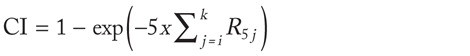
where R_5j are rates for 5-year age bands. It follows:

Taking the approximation that for X << 1 we have that 1–exp^–X ≡ X and under the assumption that RR₁₀ is constant along all the age bands considered, we obtain:

and:

Then, for ILCR we will have:

CI_TM – CI_TD = (CI₁₀ – CI_TD) × ΔE / 10 ≡ ((RR₁₀ × CI_TD) – CI_TD) × ΔE / 10 ≡

≡ CI_TD × (RR₁₀ – 1) × ΔE / 10 (11)

As an example of application of formula (11), adopting the terminology and the age-band restrictions used by Galise et al [5] we have for ILCR (Incremental Lifetime Cumulative Risk), which is the terminology used by Galise et al for excess lifetime risk (ELR):

where the index j stands for the age-bands 30–34, 35–39,. . ., 65-69, 70–74.

In this way we passed from yearly attributable cases – fomulas (3) and (10) – to excess lifetime risk. To complete the demostration and to become able to compare the excess lifetime risk (or ILCR) with USEPA (or others) action levels (10⁻⁶, 10⁻⁵, 10⁻⁴) one more step is requested.

According to USEPA the value of ELR can be computed, starting from the concept of Unit Risk (UR), with the formula:

ELR_UR = UR × ΔE

and because, using the average relative risk method [9]:

UR = CI × [(RR – 1) / X]

where × is equal to 1 when we consider an exposure lasting for the whole day, for all the days of a year, for a lifetime, we will have for ELR_UR:

ELR_UR = CI × (RR – 1) × ΔE

This formula for excess lifetime risk USEPA like (ELR_UR) has the same structural form of the ILCR obtained starting from rates of occurrence, and this suggests (under the hypothesis of validity of both the assumptions and the approximations adopted) to compute ILCR with the formula:

and to compare the resulting value with the levels of action suggested by USEPA and others (10⁻⁶, 10⁻⁵, 10⁻⁴). It is worth noting that also for ILCR it remains open the question of which R_TD do we have to use in the computations, as we have previously discussed.

Discussion

Epidemiologic HIA is receiving increasing interest in Italy, particularly because it is usually requested in the administrative procedures for the authorization of some industrial projects.

The methodology of eHIA in common use requires the knowledge of the baseline rate (R_TD) for the diseases under evaluation and of the relative risk (RR) for a unit increase of exposure. Such methodology cannot be applied when the baseline rate (R_TD) is equal to zero: to take account of this possibility we have enlarged the methodology and we have suggested formulas that use the Excess Risk (ER) indicator instead of the Relative Risk (RR). Unfortunately, information on RR are commonly available while information on ER are scarsely provided by the relevant literature: efforts should be done to overcome this limitation.

In addition, at least two questions still remain open: which rate at baseline should be used for the estimation of attributable cases, and how to use the results of eHIA (in terms of attributable cases) to take decisions regarding the realization of industrial projects. In this paper both questions have been discussed.

To motivate the discussion about which rate at baseline could be used in the estimation process an example has been provided which has to do with the Sars-CoV-2 virus diffusion. Enlarging the example, we have shown that the use as baseline for a certain disease (e.g., lung cancer) of a rate that is caused by all the risk factors for that disease (i.e., smoking, industrial pollution, traffic, heating, occupations, …) instead of a rate that is caused simply by the risk factors (for that disease) that are under evaluation (e.g., industrial pollution) significantly overestimates the number of cases attributable to the project we are speaking of, and the overestimation depends on the specific disease(s) under scrutiny: in particular it is important to know how much of the baseline rate (R_TD) is explained by risk factors that are or that are not modified by the emissions of the project (R_{TD E}, R_{TD OF}). The great majority of the projects registered on the website of the Ministry of Environment [3] in which eHIA results are presented discusses of diseases like natural mortality, cardiovascular diseases, coronary diseases, respiratory diseases, lung cancer, in connection with industrial pollution (PM, NOx): all of these diseases have many risk factors, and the majority of these risk factors has no connection (and no interaction) with industrial pollution.

To overcome this overestimation (which could be numerically very relevant: see, for example the case of pollution and lung cancer, where the value of R_TD is at least ten times the value of R_{TD E}), some efforts should be devoted to find a way (a methodology) to estimate R_{TD E}. In the meantime, prudence should be used in the interpretation of the results of eHIA, both in terms of attributable cases or in terms of Incremental Lifetime Cumulative Risk, and the documents that report eHIA results should discuss (for the diseases under scrutiny) the possible extension of this overestimation.

The use of the value of AC that has been predominantly made by the Italian national authorities in the procedures of authorization of industrial projects is crude and grossly unsatisfactory: when AC was less than 0 (which means that the implementation of a project avoids the occurrence of some cases of a disease) the authority released a positive evaluation, otherwise (i.e., when AC was > 0) the evaluation of the project was negative. If this should be the criterion for decision making it is obvious that eHIA is not necessary, and a look at ΔE is sufficient to make any decision: when ΔE is greater than zero some additional cases will be attributable to the project, and a negative evaluation will be released (and the contrary when ΔE is < 0). This logic mimics the USEPA toxicologic risk assessment for non-carcinogenic effects, where ΔE is compared to a reference concentration (RfC) and a decision is made simply with regard to the value of the ratio ΔE/RfC (less or greater than one), without any need to compute AC.

Apart from this crude approach, the results of eHIA in terms of attributable cases do not have any easy (or meaningful) interpretation: for someone the number of cases will be judged “small”, for some other the same number of cases will be judged “big”. To overcome this arbitrary and subjective judgement we need some rule, at least for decision making.

In the USEPA (and others) toxicologic risk assessment for carcinogenic effects the logic for making decisions is the following: on the one hand an estimate of an excess lifetime risk is provided; on the other hand, some levels of action are established (10⁻⁶, 10⁻⁵, 10⁻⁴). To mimic this logic Galise et al [5] suggested to compute ILCR (Incremental Lifetime Cumulative Risk) and to compare it to USEPA (and others) action levels.

In the previous section we have followed the suggestion by Galise et al and, under assumptions and approximations that must be validated in any specific situation under scrutiny, we have derived the necessary formulas and have demonstrated the possibility of the comparison between the results coming from this approach (ILCR) and the levels of action used by USEPA (and others).

Some comments regarding the assumptions and the approximations we have introduced are needed. The USEPA excess lifetime risk and action levels have been proposed for cancer while ILCR is not specific for cancer: the assumption here is that the USEPA methodology did not use specific assumptions related to cancer that we did not implement in the development of the formulas we have provided. Because ILCR has not been developed specifically for cancer it could be used with any kind of disease: in these cases the USEPA (and others) action levels are not necessarily valid and useful. For example, Galise et al compared the ILCR derived for lung cancer with the USEPA action levels which have been derived for all cancers: are they fully comparable?

With regards to the formulas we have used to pass from age-specific rates to cumulative risk, it is well known [10] that such formulas cause an overestimation of the cumulative risk.

Also the average relative risk method used to compute UR [9] has some assumptions (the relative risk is some function of cumulative exposure, there is no threshold dose for carcinogens, the linear extrapolation of the dose–response curve towards zero gives an upper-bound conservative estimate of the true risk function if the unknown (true) dose–response curve has a sigmoidal shape, the background age/cause-specific rate at any time is increased by a constant factor) that need to be verified for the exposures under evaluation. Other and more specific assumptions are listed in reference [9].

The many approximations and assumptions required by the computations suggest a prudent use of the numerical values emerging from eHIA, particularly when they are close to the action levels and the decision that has to be made is relevant. In addition, efforts to try to specify and to quantify uncertainty should be made explicit in each HIA [11].

Conclusion

General guidelines for using epidemiology in HIA, and particularly in eHIA, have been available for a long time [11], but some questions still remain open. In this paper we have derived the formulas that should be used in eHIA both to compute attributable cases (AC) and Incremental Lifetime Cumulative Risk (ILCR), and have also enlarged the methodology and the formulas in common use to consider the case in which the baseline rate (R_TD) is equal to zero: in this situation we suggest to use Excess Risk (ER) instead of Relative Risk (RR) estimates.

This paper has also shown that the use as baseline rate of the rate that is caused by all the risk factors for a disease (R_TD) can be questionable and has suggested to switch to the rate that is caused simply by the risk factors that are under evaluation (R_{TD E}). The two approaches (R_TD vs R_{TD E}) produce estimates, both of AC and of ILCR, that can be largely different, and work in this area needs to be done.

Lastly, this paper has shown that, under approximations and assumptions that need to be validated in each specific situation, ILCR can be computed and the emerging value can be compared with USEPA (and others) action levels.

Prudence and caution should be exercised in using eHIA results, particularly if strong decisions have to be made. As suggested by Schouten et al [9] on page 29: “The presented quantitative risk estimates can provide policy-makers with rough estimates of risk that may serve well as a basis for setting priorities, balancing risks and benefits, and establishing the degree of urgency of public health problems among subpopulations inadvertently exposed”.

Declaration of interests:

In the last three years, the Author has been involved in many Health Impact Assessments of industrial projects (especially power plants) in which an epidemiologic assessment was required.

References

- 1.Decreto legislativo 16 giugno 2017, n. 104: Attuazione della direttiva 2014/52/UE del Parlamento europeo e del Consiglio, del 16 aprile 2014, che modifica la direttiva 2011/92/UE, concernente la valutazione dell’impatto ambientale di determinati progetti pubblici e privati, ai sensi degli articoli 1 e 14 della legge 9 luglio 2015, n. 114. (17G00117). G.U. 6 luglio 2017, n. 156 [Google Scholar]
- 2.Dogliotti E, Achene E, Beccaloni E, et al. Linee guida per la valutazione di impatto sanitario (DL.vo 104/2017) Roma: Istituto Superiore di Sanità; 2019. (Rapporti ISTISAN 19/9) [Google Scholar]
- 3.Ministero dell’Ambiente. https://va.minambiente.it/it-IT. (last access on October, 5th 2021) [Google Scholar]
- 4.US EPA. Risk Assessment Guidance for Superfund (RAGS), Part A. Washington, US EPA, 1989 [Google Scholar]
- 5.Galise I, Serinelli M, Morabito A, et al. The Integrated Environmental Health Impact of emissions from a steel plant in Taranto and from a power plant in Brindisi, (Apulia Region, Southern Italy) Epidemiol Prev. 2019;43(5-6):329–337. doi: 10.19191/EP19.5-6.P329.102. [DOI] [PubMed] [Google Scholar]
- 6.AIRC. https://www.airc.it/cancro/informazioni-tumori/corretta-informazione/inquinamento-atmosferico. (last access on October, 5th 2021) [Google Scholar]
- 7.DM 24 aprile 2013. Disposizioni volte a stabilire i criteri metodologici utili per la redazione del rapporto di valutazione del danno sanitario (VDS) in attuazione dell’articolo 1-bis, comma 2, del decreto-legge 3 dicembre 2012, n. 207, convertito, con modificazioni, dalla legge 24 dicembre 2012, n. 231) [Google Scholar]
- 8.Kleinbaum DG, Kupper LL, Morgenstern H. Epidemiologic Research, John Wiley & Sons; 1982. [Google Scholar]
- 9.World Health Organization: Air Quality Guidelines for Europe. WHO Regional Publications, European Series No 91. Copenhagen, WHO, 2000. (Second Edition) [PubMed] [Google Scholar]
- 10.Schouten LJ, Straatman H, Kiemeney L, Verbeek A. Cancer incidence: life table risk versus cumulative risk. J Epidemiol Community Health. 1994;48(6):596–600. doi: 10.1136/jech.48.6.596. [DOI] [PMC free article] [PubMed] [Google Scholar]
- 11.World Health Organization Regional Office for Europe. Evaluation and use of epidemiological evidence for environmental health risk assessment. Guideline Document. Copenhagen, WHO Regional Office for Europe. 2000 doi: 10.1289/ehp.00108997. [DOI] [PMC free article] [PubMed] [Google Scholar]