Assembly and Analysis of Cell-Scale Membrane Envelopes

Abstract

The march towards exascale computing will enable routine molecular simulation of larger and more complex systems, e.g., simulation of entire viral particles, on the scale of approximately billions of atoms–a simulation size commensurate with a small bacterial cell. Anticipating the future hardware capabilities that will enable this type of research, and paralleling advances in experimental structural biology, efforts are currently underway to develop software tools, procedures and workflows for constructing cell-scale structures. Herein, we describe our efforts in developing and implementing an efficient and robust workflow for construction of cell-scale membrane envelopes and embedding membrane proteins into them. A new approach for construction of massive membrane structures that are stable during the simulations is built on implementing a subtractive assembly technique coupled with the development of a structure concatenation tool (fastmerge), which eliminates overlapping elements based on volumetric criteria rather than adding successive molecules to the simulation system. Using this approach, we have constructed two “protocells” consisting of MARTINI coarse-grained beads to represent cellular membranes: one the size of a cellular organelle, and another the size of a small bacterial cell. The membrane envelopes constructed here remain whole during the molecular dynamics simulations performed and exhibit water flux only through specific proteins, demonstrating the success of our methodology in creating tight cell-like membrane compartments. Extended simulations of these cell-scale structures highlight the propensity for non-specific interactions between adjacent membrane proteins leading to the formation of protein microclusters on the cell surface, an insight uniquely enabled by the scale of the simulations. We anticipate that the experiences and best practices presented here will form a basis for the next generation of cell-scale models, which will begin to address the addition of soluble proteins, nucleic acids, and small molecules essential to the function of a cell.

Graphical Abstract

1. Introduction

Advances in experimental structural biology, particularly the resolution revolution in electron microscopy,¹ coupled with development of novel cellular biophysical techniques have enabled biologists to achieve the first high-resolution views into the interior of a cell and the spatial arrangement of inner organelles and macromolecular systems necessary to its function.^2–4 Paralleling and complementing these advances, we the authors recognize a growing demand for novel computational technologies that permit users to incorporate experimental data into cell-scale molecular models and bring them to life through simulation. Computational techniques such as Molecular Dynamics (MD) Flexible Fitting (MDFF),^5,6 restrained ensemble MD (reMD),^7,8 and general restrained dynamics through arbitrary reaction coordinates^9,10 allow experimental datasets to be integrated into detailed atomistic molecular models of biological systems. Further extensions to these techniques allow for extensive sampling of protein conformational changes and folding processes central to biological function.^11,12

While studying isolated biomolecular systems computationally has proven to offer a powerful approach, sampling individual biomolecules in isolation removes them from their larger biological context. To restore this context, simulation groups have leveraged improvements in computing hardware and software to study progressively larger systems. Such holistic approaches to study representative systems at atomic detail have demonstrated the importance for taking a broad view, such as by revealing interaction networks and couplings within, e.g., photosynthetic organelles,¹³ the bacterial cytoplasm,^14,15 and biomass.¹⁶ Early simulation work on viruses^17,18 has now matured into atomic models for pathogens such as influenza¹⁹ and SARS-CoV-2.^20,21 With the impending arrival of the first exascale supercomputers, it is expected that atomic models for entire cells will become tractable simulation targets at the discovery frontier.

Constructing models at the cell-scale will require novel, robust approaches to generate accurate initial models that are numerically stable during simulation. Generating accurate models of relevance to biological living forms is challenging due to their heterogeneity, as even a minimal bacterial cell needs many different components to maintain viability.²² Current tools are mostly designed for smaller molecular systems and tailored towards handling a limited number of components, rather than, e.g., the hundreds of different proteins with varying copy numbers found in a curved membrane representing a live cell.

In realistic systems, the membrane itself is a multicomponent assembly of diverse lipids and associated proteins. These components are arranged inhomogeneously, within different cellular regions (e.g., the nucleoid) that feature locally enhanced concentrations of specific cellular components at both the organelle and metabolite levels.^23–25 Naturally, generating a full model for even a minimal cell that features all of these elements (i.e., proteins, carbohydrates, nucleic acids, salts, lipids, sterols, metabolites, etc) remains a technical challenge. However, foundational studies have already begun, including models for an “average” bacterial cytoplasm,¹⁴ and mesoscale modeling approaches as exemplified by cellPACK.^26,27

Herein we describe our contribution to efforts in cell-scale modeling by developing and implementing a method for constructing a cellular envelope composed of lipids and embedded proteins surrounding the cytoplasm, which we term a “protocell”. The method shares many of the same goals as other liposome or cell envelope generation schemes, such as TS2CG,²⁸ CHARMM-GUI,^29,30 BUMPy,³¹ or LipidWrapper,³² namely, constructing biologically relevant structures that permit their simulation. In our testing, we have generated two protocells, one with a 40-nm diameter, approximately the size of a small organelle,³³ and a larger, 200-nm-diameter protocell, approximately the size of a small bacterial cell.³⁴ We will describe in detail the steps involved in protocell construction, along with practical challenges associated with its large copy number and heterogeneity. The generated protocells remain whole during subsequent simulations despite modeling challenges posed by the membrane environment. Analysis of the resulting trajectories captures effects related to protein complex formation and diffusion at large scale, highlighting the potential for cell-scale models to describe relevant phenomena at biological length scales.

2. General Aspects of Methodology

In constructing a protocell, a major challenge is to pack the many constituents into the target geometry while ensuring the correct density and integrity of the membrane. This challenge is by and large related to generating a proper interface between membrane proteins and the surrounding lipids and other membrane components (e.g., sterols).³⁵ Close contact between the membrane components and embedded proteins, which is essential to biological function,³⁶ can be generated for individual proteins through a number of established techniques.^37–41 However, this close contact can be difficult to arrange for cell-scale systems where automation and unsupervised error checking and correction become crucial, as artifacts (e.g., ring piercing, lipid entanglements) that are rare in typical simulation systems of individual proteins (10k-1M atoms) become substantially more probable, if not commonplace.

Toolsets that are focused on common use cases–embedding a single protein into a planar bilayer⁴²–are not adequately scalable to cell-scale modeling. For example, adjacent membrane proteins at the cell scale should not overlap. The many disparate protein components within the membrane and their size hetrogeneity make it difficult to arrange the individual proteins from a priori knowledge. For soluble systems, simple geometric checks can remove clashing solvent molecules, and/or exploring alternative random protein placements can be used to avoid protein-protein overlap. However, such schemes fail for cell-scale membrane systems, whose high protein density combined with 2D confinement places strict limits on protein placement within a defined geometry. Furthermore, since individual acyl tails are long relative to water, removing whole lipid molecules to resolve steric clashes at the lipid-protein interface would introduce a non-trivial gap, which can sum to large void volumes when embedding hundreds or thousands of proteins into the membrane. Such voids can result in unstable molecular models during the ensuing simulations.

Failing to resolve steric clashes often results in ring penetration (piercing), where a lipid acyl tail pierces molecular rings, e.g., aromatic side chains or polycyclic sterols, leading to a metastable but unphysical molecular geometry and defects in dynamics for both the piercing lipid and the pierced ring. Neither ring penetrations nor large gaps can be tolerated when constructing cell-scale membrane systems, as they often rapidly lead to structural instabilities and/or lengthy initial equilibration times; however, finding and correcting these flaws can be slow as they often scale poorly with system size.^43,44

3. Protocell Construction Protocol

Our protocol for generating a protocell is outlined in Fig. 1, highlighting key steps, with details provided in subsequent sections. Briefly, we use points on a Fibonacci sphere for initial placement of the individual protein or lipid components in two separate spherical shells generated along two paths that will eventually merge into one protocell. Below, we refer to these as the lipid and protein shells/components/spheres, interchangeably. Along the protein path, the initial Fibonacci spherical placement is refined through an ultra-coarse grained (UCG) simulation, which will be backmapped to higher-resolution proteins in a later step. The resulting coordinates from the protein shell are then used in the “membrane lithography” step to determine which lipids from the lipid shell should be kept and which ones should be removed in order to avoid clashes with the protein components. The membrane-path and protein-path products are then merged together and solvated to generate the final protocell model. The methodological challenges and implementation details are laid out in subsequent sections.

Figure 1: Protocell Construction Workflow.

Protocell assembly across two overall paths. The protein path (gray arrows) prepares the protein components (multi-colored surfaces) and their tightly associated lipids (orange), by optimizing protein position through an ultra-coarse grained simulation (gray triangle) where each protein is represented by up to 4 particles (semi-transparent beads). The membrane path (purple arrows) prepares the bulk membrane lipids (purple) through membrane lithography, using the optimized positions of the protein shell components (gray dashed line) to generate a membrane mask. The membrane mask evaluates bulk lipid overlap with the protein shell (red for high overlap, blue for low overlap, white for intermediate), and selects as many lipids with minimal overlap as needed to complete the protocell. The complete protocell thus has optimally placed protein components (multi-colored surfaces), lipids tightly associated to the proteins (orange), and bulk lipids (purple).

A major challenge associated with constructing the atomic protocell models was their sheer size. Atomic models on the scale of small bacterial cells would, on the low end, be approximately a billion atoms, and their simulation would represent a substantial computational cost on available hardware. Therefore, for our tests, we constructed the molecular systems using a MARTINI v2.1 coarse-grained (CG) representation,^45–47 thereby reducing the required particle counts for the large protocell model to approximately 100 million particles - a tractable system size for existing software and hardware. However, the approach and algorithms described herein were explicitly designed with scalability in mind and an expectation that they can be easily extended to the construction of atomistic protocell models.

3.1. Protein Path

The top half of Figure 1 highlights the path for assembling the protein components of a protocell into a protein shell (spherical arrangement). The path traces the evolution for protein positions from an initial guess made by Fibonacci placement (Sec. 3.1.2) through UCG simulation (Sec. 3.1.3) to a final protein shell. However, we first need to determine the protein content for these steps (Sec. 3.1.1).

3.1.1. Selection of Protein Components

For the purpose of algorithm development, one could choose even a single integral membrane protein to fill the protocells; however, such a system would not represent the diverse shapes and sizes of membrane proteins in a cell. Instead, we selected membrane proteins identified in the minimal genome of Mycoplasma mycoides²² for which closely homologous structures are available in the Orientation of Proteins in Membranes (OPM) database^62,63 (Table 1). This is analogous to the approach taken by recent efforts to develop CellPack models for Mycoplasma mycoides.⁶⁴ Large pressure differences between the inside and outside of closed lipid structures is a well-known artifact of water placement, a problem addressed in other vesicle creation procedures by inserting pore-like structures or nanotubes into the membrane.⁶⁵ We included aquaporin water channels to help equalize osmotic gradients during the simulation. Since the true protein stoichiometry in vivo is unknown, copy numbers of individual proteins (Table 1) were determined at random. The random numbers were evaluated such that the membrane protein components would collectively occupy approximately 20% of the total membrane surface area for our protocell models, in line with estimates of the protein occupancy in red blood cell membranes.⁶⁶ The method used for determining protein surface area is detailed in Section 3.2.2. At 20% membrane occupancy, approximately half of the final protocell dry weight is composed of protein (50% for the organelle-scale, 40-nm protocell, and 46% for the cell-scale, 200-nm protocell), falling into the range (18–75% protein by weight) measured experimentally for plasma membranes of other cell types.⁶⁷ The membrane topology for each protein was adopted from the OPM database^62,63 while the initial structures for each membrane protein along with lipids within its 5 Å surrounding (lipid belt) were obtained from the MemProtMD database,⁴⁰ which provides an equilibrated structure of each protein embedded in a dipalmitoylphosphatidylcholine (DPPC) membrane.

Table 1:

Protein type and copy numbers for the 14 membrane proteins inserted into the organelle-scale (40 nm) and cell-scale (200 nm) protocell models. These structurally known proteins were chosen based on their functional and structural homology to membrane proteins identified within the minimal genome of Mycoplasma mycoides.²² The copy numbers were chosen to achieve a target occupancy of the total membrane surface area in each case. The color used for the PDB code matches the protein representation in other figures throughout the text.

PDB Code	Protein Description	Copy number
		40 nm	200 nm
1RC2 48	Aquaporin Z (AqpZ)	1	97
2VOY 49	Copper Transporter (CopA)	3	166
2XOK 50	F0/F1 ATP Synthase (ATPase)	6	63
3B5Y 51	Lipid Flippase (MsbA)	8	29
3D31 52	Molybdenum Transporter (ModBC)	3	130
3MP7 53	Translocon (SecY)	2	103
3TUJ 54	Methionine Transporter (MetNI)	8	136
3WVF 55	Membrane Chaperone (YidC)	2	126
4HUQ 56	Energy Coupling Factor (ECF)	2	117
4J7C 57	Potassium Transporter (KtrAB)	1	148
4KY0 58	Glutamate Transporter (GltTk)	6	41
4Q2E 59	Cytidine-Diphosphate Diacylglycerol Synthetase (Cds)	7	50
4S0F 60	Membrane-Bound Protease (PCAT)	5	57
4Z7F 61	Folate Transporter (FolT)	1	134

The lipid belt (orange lipids in Fig. 1) was kept to minimize ring-piercing artifacts that might arise at the interface between newly placed lipids and protein side chains. Generating an ideal interface between membrane proteins and the surrounding lipids is the primary challenge for modeling realistic cell membranes.³⁵ In this case we use MemProtMD⁴⁰ together with a distance based criterion to select the protein and surrounding lipid patch to generate protein-lipid structures with pre-equilibrated geometries.

3.1.2. Initial Protein Placement with Fibonacci Spheres

We evenly distribute N proteins on a spherical surface, following the distribution of a Fibonacci sphere, which is used in many applications to generate a set of approximately equally spaced points on a spherical surface. The set of N points (P) describing a Fibonacci sphere is defined by:

$$P(i)=\text{arccos}\left(\frac{1-2i}{N}\right)\widehat{\theta }+\frac{2\pi i}{\phi }\widehat{\varphi }.$$ (1)

Here, $\phi =\frac{1+\sqrt{5}}{2}$ is the golden ratio, and θ and φ are the polar and azimuthal angles in spherical coordinates. Since the limit of the ratio between items in the Fibonacci sequence is the golden ratio, this arrangement of points on a sphere is called a Fibonacci sphere.^68,69 The initial set of protein centers P is simple to determine from Eq. 1, resulting in the initial protein geometry shown in Fig. 1. Since some proteins are larger than others, the optimal distance between them can vary greatly; evenly distributing proteins on a sphere may result in their partial overlap in the initial configuration, especially at high protein ratios. This problem is addressed in the following section by taking advantage of UCG simulations.

3.1.3. Ultra-Coarse Graining of Membrane Proteins

To improve the unphysical initial protein arrangement that might result from Fibonacci sphere placement, we optimize the protein positions through a UCG simulation (purple box, Fig. 1). Within this simplified model, up to four UCG particles approximate the shape of each protein: two particles for the transmembrane part of the protein, and two particles for any additional domains protruding on either side of the membrane (water-soluble beads), as exemplified in Fig. 2. The two transmembrane UCG particles are centered at the level of the lipid headgroups at ±17 Å from the membrane center, one in each leaflet. Assignment of two transmembrane UCG particles will allow us to enforce and maintain the orientation of the protein in the membrane (cytoplasmic vs. extracellular) during the simulations. For proteins with substantial protrusions beyond the membrane plane (beyond ±32 Å along the membrane normal), additional UCG particles were used to represent the protrusions. The radii for all UCG particles was determined based on the maximum distance of their composing MARTINI beads from their center. The masses of all UCG particles were determined from the sum of their constituent MARTINI particles.

Figure 2:

Detailed view into the ultra-coarse graining process and simulation. To generate a 3-particle UCG representation for the copper transport protein (orange spheres, right, PDBID: 2VOY), we start from the initial protein MARTINI CG representation (left, pink and yellow solid spheres underneath the semi-transparent spheres) embedded within the membrane patch (gray, teal, and blue spheres, some not shown to enhance the visibility of the protein). Two UCG particles (bottom transparent orange spheres on the left) are defined to represent the membrane-embedded domain of the protein, one in the extracellular leaflet and one in the cytoplasmic one. The copper transporter also has a large soluble domain that protrudes on the intracellular side. The soluble domain is mapped onto a third UCG particle with radius r. During UCG simulations, only the large beads are retained (orange particles, right), with bond (black line), angle (angle hatching), and dihedral (not featured for this three-bead model) terms added to maintain the relative geometry between the UCG particles that represent the protein components. The two UCG particles that represent the transmembrane component are held at the inner and outer protocell surface by a fictional spring in the simulation, represented as black springs in the figure.

After placement, simulations of the UCG protein particles were performed with restrained dynamics to eliminate protein overlaps (gray triangle in Fig. 1). To this end, we created a CHARMM-style force field to describe the motion of these UCG particles. Note that the sole purpose of this step is to reasonably space the proteins within the spherical shell that will eventually be used as the protein component of the protocell. Bonds, bond angles, and dihedral angles between the particles (black lines and angles, Fig. 2, right) were restrained using harmonic potentials with force constants of 100 kcal mol⁻¹Å⁻² for bonds, 400 kcal mol⁻¹radian⁻² for angles, and 200 kcal mol⁻¹radian⁻² for dihedrals. The choice of relatively high force constants in this step is intended to preserve the overall shape of the proteins during this coarse adjustment stage. Equilibrium values for the bonded forces were taken from the initial geometry of the UCG particles for each protein. The non-bonded interactions were determined strictly through Lennard-Jones potentials, with the electrostatic charge on each UCG particle set to 0. For the two transmembrane UCG particles, the well depths were set to 0.6 kcal mol⁻¹, with the value for $\frac{r_{min}}{2}=20+r$, where r is the radius assigned to the particle. Similarly for particles that represent the solvent-exposed portions of the protein, the well depths were 0.3 kcal mol⁻¹, with the value for $\frac{r_{min}}{2}=10+r$. In order to maintain the spherical arrangement of the UCG particles, they were radially restrained to their initial distance from the origin (the center of the sphere) via harmonic potentials with a force constant of 25 kcal mol⁻¹Å⁻². The UCG simulations were carried out in NAMD 2.11 at 600 K and using 50-ns timesteps until the particles stopped moving 2.5 million steps later, at which point the proteins were properly distributed on the membrane envelope surface. For each protein within the system, a transformation matrix was determined between the first and last frames of the simulation. These transformation matrices were applied later to the initial MARTINI representation for each protein to generate an overlap-free protein shell (Fig. 1). The UCG simulations and backmapping to traditional MARTINI particles are analogous to the coarse-graining and backmapping approaches frequently used to achieve long timescales in membrane simulations.⁷⁰

3.2. Membrane Path

Generating a spherical membrane patch of lipids is conceptually quite simple. We drew lipids from a conformation library at random and arranged them (Sec. 3.2.1) according to the Fibonacci sphere described above. Integrating the lipid shell together with the protein shell, however, demands that the lipid counts in the upper and lower leaflets are chosen such that the surface areas of both leaflets are compatible once the proteins are added. This means that the total surface area for each leaflet needs to be computed, as well as the fraction occupied by protein. Lipids from the spherical shell that would clash with protein components are removed by computational lipid lithography, and the remaining lipids are merged with the protein shell to complete the protocell.

3.2.1. Initial Lipid Sphere Assembly with Fibonacci Spheres

Initially, the complete DPPC lipid sphere (Fig. 1 is generated through the Fibonacci sphere process introduced in Eq. 1. However, since the inner leaflet has a smaller surface area than the outer leaflet, the number of lipids in each leaflet are not equal. The initial spherical bilayer is produced by placing lipids onto points defined by two Fibonacci spheres, one for each leaflet. For a specified protocell radius, r, two Fibonacci spheres are constructed using a leaflet offset o, (−17 Å for the inner leaflet, and +17 Å for the outer leaflet). The number of lipids (N_t), that were used to construct each leaflet was then determined using the surface area of the spheres and the accepted value for the area occupied by each lipid (a_l, in this case, 65 Ų per DPPC lipid).

$$N_t=\frac{4\pi {(r+o)}^2}{a_l}$$ (2)

The two Fibonacci spheres were populated with lipids using a conformation library developed for CHARMM-GUI,⁴³ consisting of 4,000 lipid conformations, creating the lipid shell (purple) shown in Fig. 1. While in principle a similar approach could be used for mixed lipid bilayers, we choose a homogeneous DPPC lipid composition to match that of the proteins’ lipid belt around adapted from MemProtMD.⁴²

3.2.2. Protein Surface Area Determination

Not all N_t lipids in each leaflet will make it into the final system, since some of them must be removed to accommodate the protein component of the protocell. The number of lipids to remove from each leaflet is determined by the total protein surface area in that leaflet, as well as the total number of lipids in the lipid belts of proteins (N_cc) that are already present in the protein shell. The total protein surface area is determined by the product of the number of proteins (N_p), and the area per protein (A_p). Thus, the number of kept lipids in a given leaflet, N_k is determined by

$$N_k=N_t-N_{cc}-N_p{A}_p/a_l,$$ (3)

where a_l is the area per lipid. The surface area for each protein was determined by a Monte-Carlo grid examination of each protein/membrane system from MemProtMD.⁴⁰ For a 1-Å-resolution grid overlaid on the individual membrane-embedded protein system (conventional, flat bilayer with a single protein embedded) over the whole span of the membrane in the simulation box (12–15 Å from the bilayer center in each leaflet), each grid point was evaluated for its proximity to lipid or protein components. The surface area of each leaflet occupied by the protein was then computed based on the fraction of grid points where a protein particle was closest and taking into account the periodic cell dimensions:

$$A_p=\frac{N_{\mathit{\text{prot}}}}{N_{\mathit{\text{prot}}}+N_{lip}}{A}_{pbc},$$ (4)

where A_p is the total leaflet surface area occupied by a single protein, A_pbc is the area of the periodic cell for the whole membrane (protein + lipids) system, and N_prot and N_lip are the number of grid points assigned to protein and lipids, respectively.

3.2.3. Computational Membrane Lithography

The membrane lithography step removes lipids from the initial lipid shell generated in Sec. 3.2.1. The number of lipids to remove is calculated from Eq. 3. However, lipids cannot be removed arbitrarily. Instead, we select lipids that would give rise to largest physical overlaps with the protein, and therefore unphysical geometries such as ring piercing artifacts.

Lipids were ranked for removal using MDFF-associated methods initially created for computing atomic densities for CryoEM fitting.⁵ The atomic densities of the protein and its lipid belt were mapped onto the spherical lipid shell (gray dashed arrow, Fig. 1) by creating volumetric occupancy maps of all atoms within the protein shell, using the “mdffi” command of VMD⁷¹ with inputs for a 20-Å resolution and 3-Å grid spacing. The atomic densities were mapped onto the lipid shell and for each lipid atom the degree of steric clash (overlap) with proteins was quantified (red, white, and blue lipids, Fig. 1), based on which a membrane mask was generated. Individual atomic clashes were summed over all lipid atoms, creating a clash score for individual lipids that was then used to identify and rank lipids with highest overlap with the protein shell (red lipids in Fig. 1). The highest rank ”clash-lipids” are then removed until only N_k lipids remain, creating a membrane shell with holes that can be merged with the protein shell. The protein shell and the porated lipid shell are then combined into a single structure using the “fastmerge” tool described in Supporting Information, creating a complete protocell with integral membrane proteins and lipids (Fig. 1).

Prior to simulation, water molecules and NaCl were added to the system to approximate natural environment. Solvation and salination steps were carried out in a similar manner to lipid lithography, where a cubic water box enveloping the complete membrane sphere was constructed (the cubes measured 240 nm and 60 nm on a side for the 200 nm and 40 nm diameter protocells, respectively). A synthetic electron density was created from the membrane envelope, and water molecules were removed if they were within 15 Å of the membrane center or had a clash score > 10 based on the same 20 Å simulated resolution map created by the “mdffi” command, as described above. This combination of criteria was empirically found to eliminate water molecules near the solute. The criteria may also be sufficient for other scenarios where the interior of the cell is filled with other cellular constituents, although that hypothesis is not explicitly tested here. The protocell was embedded into this solvent mix using the “fastmerge” tool, yielding a solvated protocell suitable for simulation. Following the random replacement procedure used by the AutoIonize plugin from VMD,⁷¹ Na⁺ and Cl⁻ ions were randomly added by replacing water particles irrespective of their distance to other components until the full molecular system was charge neutral and the final ion concentration reached 150 mM NaCl.

4. Simulation Protocol and Analysis

To test the construction protocol, both protocell systems were simulated for 500 ns in an NPT ensemble using GROMACS^72,73 (version 2016 for the 200 nm diameter system, and version 5.1.2 for the 40 nm diameter system) with the Martini force field v2.1 for lipids⁴⁷ and proteins.⁴⁶ Prior to simulation, the systems were minimized using steepest descent until the Lennard-Jones energies were below 0. Due to clashes between lipids introduced during lipid placement, the initial minimization required double precision or employing soft-core potentials commonly used in alchemical calculations to avoid overflows in the force calculation. After minimization, the simulations were initiated using a 20-fs timesteps and an electrostatic cutoff at 11 Å with a dielectric screening constant of 15, following recommendations to increase simulation performance using the MARTINI force field.⁷⁴ The simulation was maintained at 320 K using a velocityrescaling thermostat⁷⁵ and 1-atm isotropic Parrinello-Rahman barostat⁷⁶ with a decay of 20ps. The P-LINCS method⁷⁷ was used to constrain stiff bonds defined in the protein topologies. The protein topologies were inherited from MemProtMD,⁴² and included the elastic bond network standard for MARTINI protein models.

Analyses of the resulting trajectories were carried out in VMD⁷¹ using purpose-built python scripts to leverage existing libraries such as numpy and the volumetric grid handling capabilities of MDAnalysis.⁷⁸ Membrane deformation and diffusion during simulation made simple geometric selection of water molecules inside vs. outside the protocell inaccurate. The analysis scripts were specifically developed to partition water molecules into inside and outside fractions, allowing individual water molecules to be counted and tracked as a function of time. At each snapshot a density was computed for the sphere of lipids and proteins, and voxels that could access an edge of the simulation box without crossing a region of high density were tagged as “outside-the-cell”; water molecules that were not in these voxels were defined as “inside-the-cell”.

Two-dimensional diffusion of each protein within the membrane (for the larger protocell) was computed using the Einstein relationship between mean squared displacement (MSD) and time:

$$D=\frac{\langle {\left(r_{t+\Delta t}-r_t\right)}^2\rangle }{4\Delta t},$$ (5)

where averaging is over all the protein copies of the same type, and r_t and r_t+Δt refer to the center of mass (COM) of the protein’s heavy atoms at t = t and t = t + Δt, respectively. The diffusion was effectively in two dimensions along the surface of the sphere, leading to multiplying the time by four as in planar membranes. However, since the membrane geometry was non-planar, the displacement r_t+Δt −r_t was computed in three-dimensional Cartesian space, relying on the validity of the small angle approximation to determine the extent of motion along the spherical surface. These diffusion coefficients can be compared to one another using the Saffman-Delbrück model,⁷⁹ where the diffusion is related to the radius (r) of a cylindrical element in the membrane:

$$D_{sd}=\frac{k_{B}T}{4\pi {\eta }_m}\left[\text{ln}\left(2L_{sd}{r}^{-1}\right)-\gamma \right],$$ (6)

where the diffusion D_sd is connected to a characteristic lengthscale known as the Saffman-Delbrück length, L_sd, which is itself related to the membrane surface viscosity (η_m) and the bulk viscosity of the surrounding fluid (η_f), with $L_{sd}=\frac{{\eta }_m}{2{\eta }_f}$.

Additionally, protein-protein contacts were assessed through two sets of simple geometric considerations. The first was to determine inter-protein distances by measuring the distance between the centers of masses of proteins i and j $\left(d_{ij}^{com}\right)$ and subtracting the effective radius of each protein, treating it as a disk $\left(r_i=\sqrt{\frac{{\text{protein}}_i\text{\hspace{0.17em}cross sectional area}}{\pi }}\right)$, such that:

$$d_{ij}=d_{ij}^{com}-r_i-r_j$$ (7)

The metric introduced by Eq. 7 is primarily used to determine the distance between neighboring proteins and can identify distant neighbors. While this simple distance, d_ij, provides information regarding spatial arrangement, it does not provide any information regarding the extent of protein-protein interactions. Accordingly, contact number, weighted by distance,^16,80,81 was measured to determine how close individual proteins were. The greater separation between MARTINI particles necessitated the following definition for the contact number between proteins A and B:

$$C_{AB}=\sum _{i\in A}\sum _{j\in B}\frac{1}{1+\text{exp}\left(2{\text{\hspace{0.17em}Å}}^{-1}\left(d_{ij}-7.5\text{\hspace{0.17em}Å}\right)\right)}$$ (8)

In this formalism, each particle pair i and j contributes nearly 1 to the total contact (C_AB) if their distance (d_ij) is less than 5 Å, and nearly 0 if the distance between the atoms exceeds 10 Å, smoothly interpolating between these values.

5. Results and Analysis

Two primary questions drive our analysis: does the construction protocol generate stable protocells, and what types of emergent behavior arise in these cell-scale structures? In terms of stability, the results are mixed. The larger protocell demonstrates excellent stability over the timescales simulated. However, we observe large deformations for the smaller protocell, which may prove instructive for future organelle-scale modeling efforts. Emergent behavior within the protocell simulations suggests that the embedded proteins spontaneously form multi-component assemblies at short lengthscales independent of any known specific interactions that might act as the driving force. Alternatively, we hypothesize that maximizing lipid tail entropy may drive protein clustering.

5.1. Protocell Stability Assessment

Creating vesicles or other closed membranes in silico is a delicate packing balance: overfilling a closed lipid compartment can rupture the membrane, whereas underfilling it can cause significant membrane deformations. Vesicles constructed, e.g., using the popular structure generation interface CHARMM-GUI, intentionally introduce water channels into them initially to allow water exchange between the inside and the outside of the closed compartment,^82,83 which might require additional potentials to prevent leaking of non-water small solutes. Our approach here is to carefully account for the surface area of the membrane and place water-permeable proteins in the bilayer, aiming to create a complete vesicle that is stable during an extended simulation.” Our two systems show mixed results, with pronounced membrane deformations for the organelle-scale, 40-nm protocell, most likely related to the high curvature of the system, and a stable membrane for the cell-scale, 200-nm protocell (Fig. 3). In both cases, the lipid phase of the envelope remains whole, and water permeation occurs only through specific proteins.

Figure 3:

Sequential snapshots of the 200-nm (top) and 40-nm (bottom) protocells, demonstrating the stability of the larger protocell relative to the smaller one, and an approximate timescale for the membrane deformations seen in the latter. Animations for both simulations are provided as Supporting Information. Lipids are shown as orange sticks, and the proteins as surfaces colored according to the scheme in Table 1 emphasizing their disparate shapes. Water and ions have been omitted for clarity.

The procedures used to generate the two protocells (large and small) employed identical algorithms for removing water and lipids overlapping with proteins. However, clear membrane deformations arise in the small 40-nm protocell during the simulation (Fig. 3), maintaining a continuous bilayer structure while creating a highly curved surface where the vesicle buds out (Fig. S1). By contrast, the large protocell yields a nearly spherical vesicle that minimizes the elastic curvature free energy.^84,85 The key to understanding the relationship between curvature and energetics lies in the theory put forward by Helfrich⁸⁴, where the free energy is determined by a combination of a surface integral proportional to curvature in conjunction with a volume integral proportional to the pressure difference across the bilayer.⁸⁴ The extreme membrane deformations observed in the small protocell (Figs. 3 and 4) are what would be expected from a significant pressure difference across the membrane, as it might be the case for any over- or under-filled protocell. The notion of water density imbalance as a reason for deformation is supported by total solvent flux into the protocells (Fig. 4A), which indicates greater water inflow relative to outflow. The net observed flux implies that insufficient water was placed initially inside the small 40-nm protocell (by at least 5%). The much larger interior volume of the large protocell can better accommodate the small osmotic asymmetry without deformation.

Figure 4:

Quantization and visualization of water flux across the bilayer. (A) Total cumulative water flux into and out of the individual protocells, measured both in absolute number (left axis) and as a fraction of total interior water (right axis). The red and black lines represent the outward and inward water fluxes, respectively, the difference of which is the net flux into or out of the protocell. (B) Graphical representation of where the fluxes are localized, by showing only water particles inside the protocell (blue spheres), in addition to the F1 ATPase (2XOK, yellow semitransparent surface) through which water channels form during simulation.

During system construction, we initially generated a water cube overlaid on the spherical membrane/protein system and removed water molecules too close to proteins or lipids. This process relied on the evaluation of the particle densities for the protein and lipid components over a grid, guiding removal of water particles whose overlapping score exceeded a chosen value. Fig. S2 demonstrates that the chosen exclusion value was close to optimal, with only a slight increase required to generate the additional 5% interior water we would have needed to fill the 40-nm protocell based on our net flux estimates. An alternative approach to fill the protocell with water would be to exclude particles based on their closeness to protein or lipid particles. We selected our density-based approach due to the GPU-accelerated atomic density calculations present in VMD,⁸⁶ whose speed allowed for much experimentation during method development.

Interestingly, the flux (Fig. 4A) did not take place through the aquaporins we had intentionally placed in an attempt to equalize imbalances in the water density, but rather through the center of the F0 ATPase (Fig. 4B). Since MARTINI water particles represent four water molecules, rather than one used in other CG methods,⁸⁷ the MARTINI water particles appear to be too large to transit the aquaporin pore. Our F0 ATPase model from MemProtMD⁴⁰ is missing the γ rotor subunit that would otherwise fill the space inside the ring made of α and β subunits.⁸⁸ The large pore created by this missing subunit allowed MARTINI water particles to cross the bilayer. The water flux through this unconventional mechanism highlights a fundamental limitation in our approach. Automated protein preparations such as with MemProtMD can easily miss key structural features that are essential to biological function. For models going forward, this example highlights the importance of checking the constituent membrane-embedded proteins after the initial membrane-embedding simulations to see if structural adjustments or further modeling are needed to plug these gaps within transmembrane proteins. Models built with MARTINI 3, which features newer water models and the potential for more finely mapped particles, may facilitate water permeation through the aquaporin molecules as originally intended.⁸⁹

Another aspect that requires particular care for future protocell models is accounting for the potentially extreme surface area asymmetry between the two leaflets. Particularly for protocells with a small diameter, a substantial difference in the surface area between the inner and outer membrane sides exists for purely geometrical reasons. For approximately cylindrical membrane proteins, with comparable surface areas occupied in the two leaflets of the embedding bilayer, the proportion of the protein-occupied surface area differs substantially between the two leaflets of a small protocell (e.g., 20.0% protein occupancy in the outer leaflet vs. 24.6% occupancy of the inner leaflet for the 40-nm protocell studied here, compared with 19.1% and 20.6% occupancies in case the 200-nm protocell, respectively). Furthermore, even at a protein area fraction of ~ 20% used in this study, there can be cases where soluble domains for neighboring proteins are intertwined on the inner side of the membrane, since there simply is not enough interior volume within the protocell to space out all proteins. By contrast, the larger 200-nm system allows more space between individual proteins within the membrane due to its lower curvature, reducing the overlap between neighboring proteins, though not eliminating them entirely.

The observed surface area mismatch has implications beyond the specific systems reported here. In our testing, extreme surface area mismatch prevented the construction of smaller (e.g., 10 nm diameter) protocell vesicles, as the cylindrical proteins used could not support the high curvature needed for that geometry. Furthermore, using membrane proteins taken from a minimal bacterial cell in a highly curved protocell (40 nm diameter) led to significant structural deformations of the protocell (Fig 3), suggesting that curvature mismatch can also be a major impediment to construction of small protocells. However, the protein-induced membrane curvature⁹⁰ is not the only effect in small protocells. Too extreme curvatures might allow the large soluble domains from antipodally positioned proteins to interact within the protocell cavity, further stabilizing the extreme curvature observed in the smaller protocell.

5.2. Insights from Cell-Scale Simulation

5.2.1. Diffusion and the Saffman-Delbrück model

The larger, stable protocell is instructive in allowing one to monitor collective motions of membrane components in a crowded environment at the molecular level. One of the natural analyses of the cell-scale protocell, which provides a large data set on protein motions in the membrane, is to determine how the diffusion constants of individual proteins compare against expectations from the Saffman-Delbrück model,⁷⁹ where a protein diffusion coefficient D ∝ ln(1/R). We observe that the Saffman-Delbrück model fits the observed diffusion coefficients with one notable exception, the potassium transporter (PDB 47JC), which acts appears larger than what the model predicts from its approximated transmembrane radius (Fig. 5). In this case, the cytoplasmic domain of the protein appears to have substantial membrane contacts (Fig. 5, lower inset), slowing down its diffusion. The slow diffusion may be a result of membrane-protein contacts between the juxtapositioned soluble domain and the membrane surface, increasing the effective radius of the transmembrane section of the protein well beyond the estimated radius.

Figure 5:

Saffman-Delbrück model (Eq. 6) curve fitting (grey dashed line) between observed lateral diffusion rates and effective protein radii. The Saffman-Delbrück length consistent with our fitted curve is 58nm. The approximate protein radius is computed assuming $r=\sqrt{\frac{\text{protein cross sectional area}}{\pi }}$, relating the mean protein cross sectional area within the membrane to the protein radius (r). The approximation is highly accurate for proteins like the aquaporin (PDB 1RC2) in the top inset (protein in blue, lipid components in brown), in which the membrane-interacting portion of the protein is fairly confined to the transmembrane region of the protein. This approximation breaks down if significant membrane-interacting elements exist in other parts of the protein, e.g., for the potassium transporter (PDB 47JC, lower inset), a phenomenon that increases the effective radius and slows diffusion. Individual points for each protein are labeled and colored according to the scheme in Table 1.

The critical parameter of the Saffman-Delbrück model is the scaling factor for the effective radius, also known as the Saffman-Delbrück length. Past MARTINI simulations of membrane proteins in planar bilayers have suggested a Saffman-Delbrück length of only 8.6 nm,^91,92 compared with the experimentally determined range of 100–1000 nm for membrane proteins in vesicles.^93,94 This discrepancy has been attributed to the finite size of the simulation’s periodic cell in planar bilayers, which underestimates lateral diffusion constants.^91,95,96 Since the protocell membrane is spherical rather than planar and is very large, the periodic cell size effect is expected to be reduced. Indeed our fitted Saffman-Delbrück length is 58nm, a significant improvement compared with planar MARTINI bilayers, but it still underestimates the length by a factor of two. The higher (and closer to experiment) Saffman-Delbrück length observed in the protocell highlights that specific physical properties of curved biological membranes cannot be reproduced by a conventional planar bilayer simulation with finite periodic cell dimensions.

The residual between the fitted 58nm Saffman-Delbrück length and the experimental 100–1000 nm length may be due to several reasons. MARTINI simulations are known to demonstrate accelerated dynamics, with diffusional events occurring 2–10x faster than they would in an atomistic system.⁴⁷ However, the crowded environment on the protocell surface may also impact diffusion, and may violate assumptions embedded in the Saffman-Delbrück model. Prior simulation work on planar bilayers and using (single-pass) proteins smaller than those included in our protocell has demonstrated decreased diffusion with increased protein concentration.^97,98 Compared with those simulations, where the protein:lipid molar ratio was as high as 1:50,⁹⁷ the operating protein concentration in our protocells is significantly lower, with approximately 220 DPPC lipids per protein in the larger protocell (309,751 lipids vs. 1,397 proteins). Thus, despite the possible limitations of the Saffman-Delbrück model in our crowded membrane, we think it is a reasonable model to describe diffusive behavior within the assembled protocells.

5.2.2. Cluster Formation at the Protocell Scale

The large length scales afforded by protocell simulation allow a unique window into protein domain formation, as shown in Fig. 3 and in the animation provided as Supporting Information. Protein clustering has been noted in prior MARTINI simulations, with stringy protein assemblies identified across multiple systems.^35,99–105 The MARTINI model used here also has been shown to overstabilize dimers for single-pass transmembrane proteins.¹⁰⁶ While prior simulations focused on replicating clustering seen experimentally, no clustering was expected a priori in our protocell simulations, as co-localization for the diverse protein set used within the protocell had not been reported experimentally. Notably, individual proteins were initially well-spaced around the protocell, with the nearest neighbors always at least 20 Å apart as measured by Eq. 7 (Fig. 6A). During simulation, clustering emerged as the nearest neighbors move closer (Fig. 6B), with many measured to be nearly touching by the end of the simulation (Fig. 6A). While the nearest neighbors get closer, the distance to more distant neighbors increases on average over the course of the simulation, suggesting the formation of only small clusters during the process, rather than large protein-enriched domains. Identifying contributing factors that facilitate small cluster formation may provide hints for protein complex organization and assembly.

Figure 6:

(A) Inter-protein distance distribution at the start and end of the 200-nm protocell simulation. (B) Evolution of the mean protein-protein distances over time. The distances between the geometric centers of proteins for the 10 nearest proteins after subtracting the radii of the two proteins were used for this analysis (Eq. 7). In (A), the distances are binned (semi-transparent bars) and fit to Gaussian distributions (solid lines). (B) reports the time evolution of the mean of the fitted Gaussians (solid lines), as well as its width (semitransparent regions on either side of the solid lines). The chosen corresponding colors in subpanels A and B are arbitrary.

Further evidence for small cluster formation is provided by cluster analysis over the course of the simulation in comparison to the initial structure (Fig. 7A & B). Initially separated proteins are observed to associate with one another during the simulation (Fig. 7C–F). Many identified clusters are quite small, consisting primarily of protein pairs, rather than large protein domains. Similar small aggregation phenomena have been observed in simulation of membrane proteins in planar bilayers.^{35,99–106,108} We note the distance between the geometric centers of neighboring proteins can be influenced by large intra- and extra-cellular domains. Thus, this metric tends to over-estimate the distance of closest approach between proteins, and may therefore hide interactions between adjacent proteins.

Figure 7:

Formation of small clusters of membrane proteins during protocell simulation. (A) The initial graph representation for proteins in the 200-nm protocell at t = 0. Each circle within the graph represents a single protein, scaled in proportion to the approximate protein radius, and colored according to the scheme in Table 1. Black lines between protein circles are drawn if the radius-adjusted distance is less than 30 Å. The placement of the individual circles in the graph is arbitrary and was carried out using GraphViz.¹⁰⁷ (B) The same data for the 200-nm protocell at t = 500ns. Within this panel, two selected clusters are highlighted (by orange and pink outlines). The molecular configurations at the initial (t = 0) and final (t = 500ns) states for these regions are shown in panels (C-F). The corresponding clusters are indicated by the borders, with (C) and (D) showing the outlined orange cluster, and (E) and (F) showing the pink cluster. Panels (C) and (E) show initial states at t = 0, while panels (D) and (F) show the final configuration at t = 500ns. Within panels (C-F), proteins are colored consistent with the scheme in Table 1. Lighter coloration indicates proteins in the vicinity that are not part of the cluster.

An alternative metric for clustering is the protein contacts (Eq. 8) measured by pairwise distance comparisons between individual proteins. This metric identifies close neighbors by contacts between them rather than the coarse geometric proximity of the protein centers (Fig. 8). What stands out from this alternative neighbor identification is that the potassium transporter included in the simulation (PDB 4J7C, purple), increases its connectivity substantially relative to a center-based clustering, as do many other protein components with substantial soluble domains. An analysis of the pairwise contacts, Table S1, indicates that the potassium transporter on its own accounts for 30% of all contacts observed in the protocell, despite making up only 10% of all proteins in it. Conversely, the aquaporin (PDB 1RC2, blue), which is featured prominently in clusters that already exist at t = 0 (Fig. 7), is a relatively minor contributor to direct protein-protein contacts, with many uncoordinated nodes (Fig. 8), and only contributing 1% to the total contacts (Table S1). The primary structural difference between these two examples is the presence (potassium transporter) or absence (aquaporin) of large soluble domains, whose nonspecific interactions may drive membrane protein co-localization. This conclusion is consistent with prior literature, where soluble domains of many tested interaction partners are shown to drive their association,^99,101–105 particularly for G-protein coupled receptors.^{101–103,105}

Figure 8:

End state clusters for the 200-nm protocell, where the number of contacts between two nodes (proteins) is represented by the thickness of the black line connecting them on the graph. Nodes have radii proportional to the radii of the proteins they represent and follow the colors scheme in Table 1. The layout in this figure is the result of the ForceAtlas2 algorithm,¹⁰⁹ as implemented in Gephi.¹¹⁰ An animation showing how the connectivity changes over the simulation time is presented as Supporting Information.

One obvious question is whether our contacts have converged over the relatively short (500ns) protocell simulations, especially for the larger one. As shown in Fig. 9A, the contacts increase at a continuously decreasing rate, which we fit to an exponential with a time constant of ~670 ns. Clearly, the contact number observed for the larger protocell has not yet converged in the performed simulation time; however, based on an exponential fit, we estimate that at the infinite time limit there would be approximately 160,000 contacts across the entire protocell, corresponding to more than 100 contacts per protein.

Figure 9:

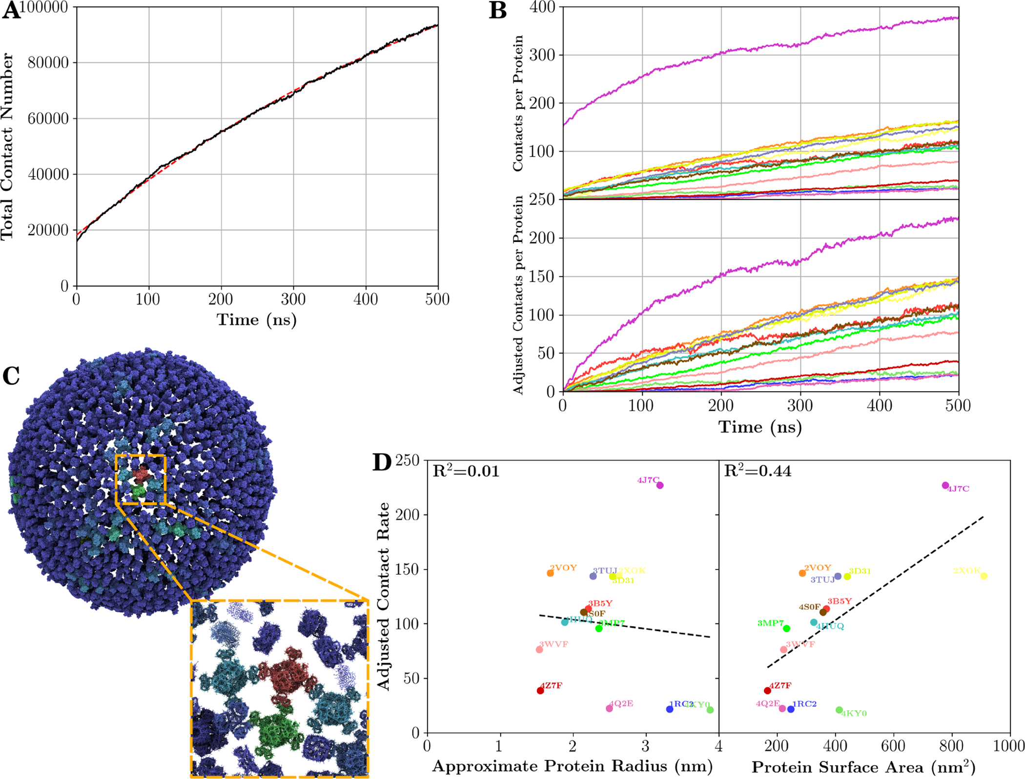
Expanded contact analysis. (A) The number of inter-protein contacts over the course of the simulation (black line), as well as an exponential fit of data (dashed red line). The fitted equation is of the form $A+B\left(1-\text{exp}\left(\frac{-t}{C}\right)\right)$, with fitted parameters A = 1.8 × 10⁴, B = 14.3 × 10⁴, and C = 670ns. (B) The mean number of contacts per protein type (top), and values after subtracting contacts present at the start of simulation (bottom). Here each line represents a different protein type, with a color scheme consistent with Table 1. The contacts formed over the course of the simulation are the preferred metric due to examples shown in (C), which displays the number of contacts present at the start of simulation (bluer colors for fewer contacts, and redder colors representing more contacts). During the protein placement step, the “wings” of the potassium transporter occasionally overlap with neighboring wings, greatly increasing the contact number in the starting model for the simulation, and potentially leading to tangled proteins (inset). (D) Relationship between the adjusted contact rate (contacts/protein) at t = 500ns and the radius of the transmembrane portion of the protein (left), or the surface area of the entire protein, including soluble domains (right). To aid the reader, a black dashed trendline is drawn through each data set, and its correlation coefficient (R) to the data is reported. Each point is colored according to the color scheme in Table 1.

Not all proteins contribute equally to the overall number of contacts. Certain proteins are much more effective than others in serving as aggregation sites, particularly the potassium transporter (Fig. 9B, Table S1). In part, this is due to the “wings” on the soluble domain of the protein making contacts with neighbors already at the start of the simulation (Fig. 9C), which reflects a shortcoming of our placement methodology, where the radius of gyration for soluble domains was used to determine the size of the additional UCG beads. However, even if contacts resulting from the initial placement are excluded (lower panel of Fig. 9B), the potassium transporter is shown to establish the most contacts during the simulation. In aggregate, contacts are poorly correlated with the transmembrane radius of a protein, but instead correlate better with the total protein surface area, including the soluble domains (Fig. 9D, right side). This further supports the idea that the soluble domains of membrane proteins, which contribute to the surface area but involve no additional lipid displacement, contribute to the observed aggregation and cluster formation.

Surface area, however, is not a perfect proxy for interaction propensity. For instance, the ATP synthase (PDB 2XOK) has a very large surface area due to its soluble domain, but because of how tall its soluble domain is, very little of that surface area can be in proximity to other interaction partners within the membrane. Similarly, the large width of the trimeric glutamate transporter (PDB 4KY0) means that the large top and bottom surfaces are inaccessible to neighboring membrane proteins. A more appropriate metric would account for such inaccessible surface area, although no robust adjustment was determined based on available data due to the large variation in protein structures within our protocell.

5.3. Comparison to Other Tools

As mentioned previously, other tools have been developed to generate protocell-like structures, each with a different design philosophy.^28–32 The highlighted tools are all able to build lipid envelopes, some with greater accessibility to more complex geometries. TS2GC²⁸ or LipidWrapper,³² for example, tesselate small planar bilayers into a larger geometry, offering the ability to generate highly complex membrane geometries. Similarly, BUMPy uses geometrical transformations to curve a planar bilayer into the desired shape.³¹ The initial spherical lipid placement from CHARMM-GUI²⁹ is most similar to what we do here, with some inspiration from PackMol¹¹¹ to restrain the lipids to a spherical geometry.

Computationally, many of these methods at large scales has proven quite efficient. TS2GC²⁸ has demonstrated scaling to 80 million particles, while PackMol has been used to build Zika virus models¹¹² and LipidWrapper³² has been used in the generation of viral envelopes at the 100-million atom scale.^19,21,113 CHARMM-GUI has fewer large systems constructed to date, possibly due to algorithmic limitations. CHARMM-GUI depends on the Torsion Angle Molecular Dynamics module, which is limited to a single CPU, creating an obvious bottleneck for large scale simulation. In building our protocells, the initial placement was computationally simple, and structural corrections could be parallelized over multiple compute elements by leveraging the spatial decomposition schemes built into MD simulation engines.

While lipid placement and parallel efficiency for all methods can be viewed sufficient for scientific use, we note that very few examples exist within the literature for a large membrane-bound structure with embedded proteins. Prior large-scale simulations for organelles¹³ or viruses^19,21,113 have often depended explicitly on available structural data for initial protein placement. For viral systems or small organelles, individual proteins are often identifiable, e.g., from cryo-tomography, facilitating initial protein placement. Lacking a tomographic guide, UCG simulations as detailed here are efficient in spacing apart a large and heterogeneous set of membrane proteins, in order to avoid entanglements. Among alternative approaches, tesselation methods can similarly reduce entanglements, but take additional care to accommodate membrane components with varying sizes and shapes. The paucity of tightly packed protcells with proteins of arbitrary shapes and sizes in the literature reflects the challenges associated with their construction, and techniques described in our approach may offer unique/alternative solutions to some of these challenges paving further the way towards generating viable protocell structures.

6. Conclusion

Here we present a protocol for constructing spherical membranes composed of large copy numbers of lipids and proteins, termed protocells. The protocol employs several steps of modeling and MD simulations along with additional implemented algorithms to ensure an optimal arrangement of the membrane components, allowing for faster equilibration and higher stability of the final model. Using this protocol, we modeled and simulated two protocell models, one at an organelle scale (40 nm diameter) and the other at a cell scale (200 nm diameter).

The findings from both protocell simulations highlight how membrane curvature may play into diffusion and protein organization at the cellular scale. The emergent phenomena from simulations at this scale hint at the biophysics to be explored beyond what is possible with an isolated protein in a planar bilayer. Moving away from studying individual proteins within a planar bilayer and instead placing membrane proteins on curved surfaces is a better representation of proteins in their native environment, as evidenced by the significant improvement of protein diffusion within protocells when compared to experiment. The 200-nm, cell-scale protocell generated here, despite its limitations, is of sufficient quality to begin to probe these questions. From the insight already present in our models, it is clear that the protocells represent a good start in developing simulation-ready membrane-protein systems.

The construction of these systems, however, remains challenging, and there are certainly areas for improvement that future investigators should pursue. Assembly processes for large-scale systems need to have linear time algorithmic complexities. The subtractive assembly procedure presented here, where holes are effectively “etched” into spherical lipid surfaces by densities calculated from protein structures fits that description, as do tesselation approaches featured in other codes.^28,32 Indeed, it may prove beneficial to combine tesselation and subtractive approaches going forward, generating lipid shells via tesselation before embedding proteins via subtractive methods. The subtractive assembly is made possible by the “fastmerge” tool, which permits large structures to be concatenated together in a memory-efficient way, approximately halving the memory footprint of the merging step. However, given the initial overlaps seen in the model, we must conclude that our UCG parameters were insufficient to ensure that each protein-lipid complex was well separated when operating at physiological protein coverages of approximately 20% of the membrane surface area.⁶⁶

Numerous potential avenues exist for improving protocell construction methods. The ultra coarse-graining process for protein soluble domains may require more particles to account for nonspherical geometries. Protein-protein contact numbers (Fig. 9) should be checked before the simulation rather than only as a post-processing step. The UCG simulations may also benefit from using purely repulsive potentials rather than standard LJ-type potentials to describe the non-bonded interactions between the UCG particles. Additionally, equilibrium simulations of the membrane proteins should be dutifully checked to ensure the water-tightness of individual membrane protein models prior to their use within the membrane envelope.

While these challenges are addressed and the next generation of cell-scale membrane models are created, the current models hint at new physics that emerges only at the cellular scale. Based on the cell-scale protocell, we observe that membrane proteins will aggregate to form small-sized clusters, independent of any specific interaction, due to entropic considerations of transitioning water and lipids from an interface into bulk. This simple explanation may contribute to the heterogeneous distribution of membrane proteins in living cells,¹¹⁴ beyond the roles of, e.g., the cellular cytoskelton¹¹⁵ or membrane cholesterol.¹¹⁶ In addition, by transitioning from a planar bilayer to a spherical one, the motion of proteins ameliorates artifacts induced by periodic boundary conditions.^91,95,96 These insights would have been impossible at the smaller scale of typical single-copy planar membrane simulations, or even at a small protocell, and highlight the unexpected observations that arise as the field pushes the boundary of the possible towards larger and more complete descriptions of biological systems.⁶⁴

Data and Software Availability

The fastmerge tool is available from github (https://github.com/jvermaas/fastmerge).

The directory structure used to build these systems has been uploaded to zenodo (https://doi.org/10.5281/zenodo.5338509).

References

- (1).Kuhlbrandt W The Resolution Revolution. Science (80-.). 2014, 343, 1443–1444, DOI: 10.1126/science.1251652. [DOI] [PubMed] [Google Scholar]
- (2).Wietrzynski W; Schaffer M; Tegunov D; Albert S; Kanazawa A; Plitzko JM; Baumeister W; Engel BD Charting the native architecture of Chlamydomonas thylakoid membranes with single-molecule precision. Elife 2020, 9, DOI: 10.7554/eLife.53740. [DOI] [PMC free article] [PubMed] [Google Scholar]
- (3).Dong D; Huang X; Li L; Mao H; Mo Y; Zhang G; Zhang Z; Shen J; Liu W; Wu Z; Liu G; Liu Y; Yang H; Gong Q; Shi K; Chen L Super-resolution fluorescence-assisted diffraction computational tomography reveals the three-dimensional landscape of the cellular organelle interactome. Light Sci. Appl 2020, 9, 11, DOI: 10.1038/s41377-020-0249-4. [DOI] [PMC free article] [PubMed] [Google Scholar]
- (4).Chambers JE; Kubánková M; Huber RG; López-Duarte I; Avezov E; Bond PJ; Marciniak SJ; Kuimova MK An Optical Technique for Mapping Microviscosity Dynamics in Cellular Organelles. ACS Nano 2018, 12, 4398–4407, DOI: 10.1021/acsnano.8b00177. [DOI] [PubMed] [Google Scholar]
- (5).Trabuco LG; Villa E; Schreiner E; Harrison CB; Schulten K Molecular dynamics flexible fitting: A practical guide to combine cryo-electron microscopy and X-ray crystallography. Methods 2009, 49, 174–180, DOI: 10.1016/j.ymeth.2009.04.005. [DOI] [PMC free article] [PubMed] [Google Scholar]
- (6).McGreevy R; Singharoy A; Li Q; Zhang J; Xu D; Perozo E; Schulten K xMDFF: molecular dynamics flexible fitting of low-resolution X-ray structures. Acta Crystallogr. Sect. D Biol. Crystallogr 2014, 70, 2344–2355, DOI: 10.1107/S1399004714013856. [DOI] [PMC free article] [PubMed] [Google Scholar]
- (7).Islam SM; Stein RA; Mchaourab HS; Roux B Structural Refinement from Restrained-Ensemble Simulations Based on EPR/DEER Data: Application to T4 Lysozyme. J. Phys. Chem. B 2013, 117, 4740–4754, DOI: 10.1021/jp311723a. [DOI] [PMC free article] [PubMed] [Google Scholar]
- (8).Shen R; Han W; Fiorin G; Islam SM; Schulten K; Roux B Structural Refinement of Proteins by Restrained Molecular Dynamics Simulations with Non-interacting Molecular Fragments. PLOS Comput. Biol 2015, 11, e1004368, DOI: 10.1371/journal.pcbi.1004368. [DOI] [PMC free article] [PubMed] [Google Scholar]
- (9).Fiorin G; Klein ML; Hénin J Using Collective Variables to Drive Molecular Dynamics Simulations. Molecular Physics 2013, 111, 3345–3362, DOI: 10.1080/00268976.2013.813594. [DOI] [Google Scholar]
- (10).Tribello GA; Bonomi M; Branduardi D; Camilloni C; Bussi G PLUMED 2: New feathers for an old bird. Comput. Phys. Commun 2014, 185, 604–613, DOI: 10.1016/j.cpc.2013.09.018. [DOI] [Google Scholar]
- (11).Orellana L Large-Scale Conformational Changes and Protein Function: Breaking the in silico Barrier. Front. Mol. Biosci 2019, 6, DOI: 10.3389/fmolb.2019.00117. [DOI] [PMC free article] [PubMed] [Google Scholar]
- (12).Hollingsworth SA; Dror RO Molecular Dynamics Simulation for All. Neuron 2018, 99, 1129–1143, DOI: 10.1016/j.neuron.2018.08.011. [DOI] [PMC free article] [PubMed] [Google Scholar]
- (13).Singharoy A; Maffeo C; Delgado-Magnero KH; Swainsbury DJ; Sener M; Kleinekathöfer U; Vant JW; Nguyen J; Hitchcock A; Isralewitz B; Teo I; Chandler DE; Stone JE; Phillips JC; Pogorelov TV; Mallus MI; Chipot C; Luthey-Schulten Z; Tieleman DP; Hunter CN; Tajkhorshid E; Aksimentiev A; Schulten K Atoms to Phenotypes: Molecular Design Principles of Cellular Energy Metabolism. Cell 2019, 179, 1098–1111. e23, DOI: 10.1016/j.cell.2019.10.021. [DOI] [PMC free article] [PubMed] [Google Scholar]
- (14).Feig M; Harada R; Mori T; Yu I; Takahashi K; Sugita Y Complete Atomistic Model of a Bacterial Cytoplasm for Integrating Physics, Biochemistry, and Systems Biology. Journal of Molecular Graphics and Modelling 2015, 58, 1–9, DOI: 10.1016/j.jmgm.2015.02.004. [DOI] [PMC free article] [PubMed] [Google Scholar]
- (15).Yu I; Mori T; Ando T; Harada R; Jung J; Sugita Y; Feig M Biomolecular interactions modulate macromolecular structure and dynamics in atomistic model of a bacterial cytoplasm. Elife 2016, 5, DOI: 10.7554/eLife.19274. [DOI] [PMC free article] [PubMed] [Google Scholar]
- (16).Vermaas JV; Petridis L; Qi X; Schulz R; Lindner B; Smith JC Mechanism of Lignin Inhibition of Enzymatic Biomass Deconstruction. Biotechnology for Biofuels 2015, 8, 217, DOI: 10.1186/s13068-015-0379-8. [DOI] [PMC free article] [PubMed] [Google Scholar]
- (17).Reddy T; Shorthouse D; Parton DL; Jefferys E; Fowler PW; Chavent M; Baaden M; Sansom MS Nothing to Sneeze at: A Dynamic and Integrative Computational Model of an Influenza a Virion. Structure 2015, 23, 584–597, DOI: 10.1016/j.str.2014.12.019. [DOI] [PMC free article] [PubMed] [Google Scholar]
- (18).Zhao G; Perilla JR; Yufenyuy EL; Meng X; Chen B; Ning J; Ahn J; Gronenborn AM; Schulten K; Aiken C; Zhang P Mature HIV-1 Capsid Structure by Cryo-Electron Microscopy and All-Atom Molecular Dynamics. Nature 2013, 497, 643–646, DOI: 10.1038/nature12162. [DOI] [PMC free article] [PubMed] [Google Scholar]
- (19).Durrant JD; Kochanek SE; Casalino L; Ieong PU; Dommer AC; Amaro RE Mesoscale All-Atom Influenza Virus Simulations Suggest New Substrate Binding Mechanism. ACS Cent. Sci 2020, 6, 189–196, DOI: 10.1021/acscentsci.9b01071. [DOI] [PMC free article] [PubMed] [Google Scholar]
- (20).Yu A; Pak AJ; He P; Monje-Galvan V; Casalino L; Gaieb Z; Dommer AC; Amaro RE; Voth GA A multiscale coarse-grained model of the SARS-CoV-2 virion. Biophys. J 2021, 120, 1097–1104, DOI: 10.1016/j.bpj.2020.10.048. [DOI] [PMC free article] [PubMed] [Google Scholar]
- (21).Casalino L; Dommer AC; Gaieb Z; Barros EP; Sztain T; Ahn S-H; Trifan A; Brace A; Bogetti AT; Clyde A; Ma H; Lee H; Turilli M; Khalid S; Chong LT; Simmerling C; Hardy DJ; Maia JD; Phillips JC; Kurth T; Stern AC; Huang L; McCalpin JD; Tatineni M; Gibbs T; Stone JE; Jha S; Ramanathan A; Amaro RE AI-driven multiscale simulations illuminate mechanisms of SARS-CoV-2 spike dynamics. Int. J. High Perform. Comput. Appl 2021, 35, 432–451, DOI: 10.1177/10943420211006452. [DOI] [PMC free article] [PubMed] [Google Scholar]
- (22).Hutchison CA; Chuang R-Y; Noskov VN; Assad-Garcia N; Deerinck TJ; Ellisman MH; Gill J; Kannan K; Karas BJ; Ma L; Pelletier JF; Qi Z-Q; Richter RA; Strychalski EA; Sun L; Suzuki Y; Tsvetanova B; Wise KS; Smith HO; Glass JI; Merryman C; Gibson DG; Venter JC Design and Synthesis of a Minimal Bacterial Genome. Science 2016, 351, aad6253–aad6253, DOI: 10.1126/science.aad6253. [DOI] [PubMed] [Google Scholar]
- (23).Stolee JA; Shrestha B; Mengistu G; Vertes A Observation of Subcellular Metabolite Gradients in Single Cells by Laser Ablation Electrospray Ionization Mass Spectrometry. Angewandte Chemie International Edition 2012, 51, 10386–10389, DOI: 10.1002/anie.201205436. [DOI] [PubMed] [Google Scholar]
- (24).Dogterom M; Surrey T Microtubule Organization in Vitro. Current Opinion in Cell Biology 2013, 25, 23–29, DOI: 10.1016/j.ceb.2012.12.002. [DOI] [PubMed] [Google Scholar]
- (25).Paparelli L; Corthout N; Pavie B; Wakefield DL; Sannerud R; Jovanovic-Talisman T; Annaert W; Munck S Inhomogeneity Based Characterization of Distribution Patterns on the Plasma Membrane. PLOS Computational Biology 2016, 12, e1005095, DOI: 10.1371/journal.pcbi.1005095. [DOI] [PMC free article] [PubMed] [Google Scholar]
- (26).Johnson GT; Autin L; Al-Alusi M; Goodsell DS; Sanner MF; Olson AJ cellPACK: A Virtual Mesoscope to Model and Visualize Structural Systems Biology. Nature Methods 2014, 12, 85–91, DOI: 10.1038/nmeth.3204. [DOI] [PMC free article] [PubMed] [Google Scholar]
- (27).Johnson GT; Goodsell DS; Autin L; Forli S; Sanner MF; Olson AJ 3D Molecular Models of Whole HIV-1 Virions Generated with cellPACK. Faraday Discuss. 2014, 169, 23–44, DOI: 10.1039/C4FD00017J. [DOI] [PMC free article] [PubMed] [Google Scholar]
- (28).Pezeshkian W; König M; Wassenaar TA; Marrink SJ Backmapping triangulated surfaces to coarse-grained membrane models. Nat. Commun 2020, 11, 2296, DOI: 10.1038/s41467-020-16094-y. [DOI] [PMC free article] [PubMed] [Google Scholar]
- (29).Hsu P; Bruininks BMH; Jefferies D; Cesar Telles de Souza P; Lee J; Patel DS; Marrink SJ; Qi Y; Khalid S; Im W CHARMM-GUI Martini Maker for modeling and simulation of complex bacterial membranes with lipopolysaccharides. J. Comput. Chem 2017, 38, 2354–2363, DOI: 10.1002/jcc.24895. [DOI] [PMC free article] [PubMed] [Google Scholar]
- (30).Park S; Choi YK; Kim S; Lee J; Im W CHARMM-GUI Membrane Builder for Lipid Nanoparticles with Ionizable Cationic Lipids and PEGylated Lipids. J. Chem. Inf. Model 2021, 61, 5192–5202, DOI: 10.1021/acs.jcim.1c00770. [DOI] [PMC free article] [PubMed] [Google Scholar]
- (31).Boyd KJ; May ER BUMPy: A Model-Independent Tool for Constructing Lipid Bilayers of Varying Curvature and Composition. J. Chem. Theory Comput 2018, 14, 6642–6652, DOI: 10.1021/acs.jctc.8b00765. [DOI] [PMC free article] [PubMed] [Google Scholar]
- (32).Durrant JD; Amaro RE LipidWrapper: An Algorithm for Generating Large-Scale Membrane Models of Arbitrary Geometry. PLoS Comput. Biol 2014, 10, e1003720, DOI: 10.1371/journal.pcbi.1003720. [DOI] [PMC free article] [PubMed] [Google Scholar]
- (33).Takamori S; Holt M; Stenius K; Lemke EA; Grønborg M; Riedel D; Urlaub H; Schenck S; Brügger B; Ringler P; Müller SA; Rammner B; Gräter F; Hub JS; De Groot BL; Mieskes G; Moriyama Y; Klingauf J; Grubmüller H; Heuser J; Wieland F; Jahn R Molecular Anatomy of a Trafficking Organelle. Cell 2006, 127, 831–846, DOI: 10.1016/j.cell.2006.10.030. [DOI] [PubMed] [Google Scholar]
- (34).Luef B; Frischkorn KR; Wrighton KC; Holman H-YN; Birarda G; Thomas BC; Singh A; Williams KH; Siegerist CE; Tringe SG; Downing KH; Comolli LR; Banfield JF Diverse Uncultivated Ultra-Small Bacterial Cells in Groundwater. Nature Communications 2015, 6, 6372, DOI: 10.1038/ncomms7372. [DOI] [PubMed] [Google Scholar]
- (35).Marrink SJ; Corradi V; Souza PC; Ingólfsson HI; Tieleman DP; Sansom MS Computational Modeling of Realistic Cell Membranes. Chem. Rev 2019, 119, 6184–6226, DOI: 10.1021/acs.chemrev.8b00460. [DOI] [PMC free article] [PubMed] [Google Scholar]
- (36).Martens C; Shekhar M; Borysik AJ; Lau AM; Reading E; Tajkhorshid E; Booth PJ; Politis A Direct protein-lipid interactions shape the conformational landscape of secondary transporters. Nat. Commun 2018, 9, 4151, DOI: 10.1038/s41467-018-06704-1. [DOI] [PMC free article] [PubMed] [Google Scholar]
- (37).Jo S; Kim T; Im W Automated Builder and Database of Protein/Membrane Complexes for Molecular Dynamics Simulations. PLoS ONE 2007, 2, e880, DOI: 10.1371/journal.pone.0000880. [DOI] [PMC free article] [PubMed] [Google Scholar]
- (38).Wolf MG; Hoefling M; Aponte-Santamaría C; Grubmüller H; Groenhof G G membed: Efficient Insertion of a Membrane Protein into an Equilibrated Lipid Bilayer with Minimal Perturbation. Journal of Computational Chemistry 2010, 31, 2169–2174, DOI: 10.1002/jcc.21507. [DOI] [PubMed] [Google Scholar]
- (39).Javanainen M Universal Method for Embedding Proteins into Complex Lipid Bilayers for Molecular Dynamics Simulations. Journal of Chemical Theory and Computation 2014, 10, 2577–2582, DOI: 10.1021/ct500046e. [DOI] [PubMed] [Google Scholar]
- (40).Stansfeld PJ; Goose JE; Caffrey M; Carpenter EP; Parker JL; Newstead S; Sansom MS MemProtMD: Automated Insertion of Membrane Protein Structures into Explicit Lipid Membranes. Structure 2015, 23, 1350–1361, DOI: 10.1016/j.str.2015.05.006. [DOI] [PMC free article] [PubMed] [Google Scholar]
- (41).Jefferys E; Sands ZA; Shi J; Sansom MSP; Fowler PW Alchembed: A Computational Method for Incorporating Multiple Proteins into Complex Lipid Geometries. Journal of Chemical Theory and Computation 2015, 11, 2743–2754, DOI: 10.1021/ct501111d. [DOI] [PMC free article] [PubMed] [Google Scholar]
- (42).Stansfeld PJ Computational studies of membrane proteins: from sequence to structure to simulation. Curr. Opin. Struct. Biol 2017, 45, 133–141, DOI: 10.1016/j.sbi.2017.04.004. [DOI] [PubMed] [Google Scholar]
- (43).Wu EL; Cheng X; Jo S; Rui H; Song KC; Dávila-Contreras EM; Qi Y; Lee J; Monje-Galvan V; Venable RM; Klauda JB; Im W CHARMM-GUI Membrane Builder toward Realistic Biological Membrane Simulations. Journal of Computational Chemistry 2014, 35, 1997–2004, DOI: 10.1002/jcc.23702. [DOI] [PMC free article] [PubMed] [Google Scholar]
- (44).Vermaas JV; Dellon LD; Broadbelt LJ; Beckham GT; Crowley MF Automated Transformation of Lignin Topologies into Atomic Structures with LigninBuilder. ACS Sustain. Chem. Eng 2019, 7, 3443–3453, DOI: 10.1021/acssuschemeng.8b05665. [DOI] [Google Scholar]
- (45).Marrink SJ; Tieleman DP Perspective on the Martini Model. Chemical Society Reviews 2013, 42, 6801, DOI: 10.1039/c3cs60093a. [DOI] [PubMed] [Google Scholar]
- (46).Monticelli L; Kandasamy SK; Periole X; Larson RG; Tieleman DP; Marrink S-J The MARTINI Coarse-Grained Force Field: Extension to Proteins. Journal of Chemical Theory and Computation 2008, 4, 819–834, DOI: 10.1021/ct700324x. [DOI] [PubMed] [Google Scholar]
- (47).Marrink SJ; Risselada HJ; Yefimov S; Tieleman DP; de Vries AH The MARTINI Force Field: Coarse Grained Model for Biomolecular Simulations. The Journal of Physical Chemistry B 2007, 111, 7812–7824, DOI: 10.1021/jp071097f. [DOI] [PubMed] [Google Scholar]
- (48).Savage DF; Egea PF; Robles-Colmenares Y; O’Connell Joseph D. III,; Stroud RM Architecture and Selectivity in Aquaporins: 2.5 Å X-Ray Structure of Aquaporin Z. PLoS Biology 2003, 1, e72, DOI: 10.1371/journal.pbio.0000072. [DOI] [PMC free article] [PubMed] [Google Scholar]
- (49).Wu C-C; Rice WJ; Stokes DL Structure of a Copper Pump Suggests a Regulatory Role for Its Metal-Binding Domain. Structure 2008, 16, 976–985, DOI: 10.1016/j.str.2008.02.025. [DOI] [PMC free article] [PubMed] [Google Scholar]
- (50).Stock D; Leslie AG; Walker JE Molecular Architecture of the Rotary Motor in ATP Synthase. Science 1999, 286, 1700–1705. [DOI] [PubMed] [Google Scholar]
- (51).Ward A; Reyes CL; Yu J; Roth CB; Chang G Flexibility in the ABC Transporter MsbA: Alternating Access with a Twist. Proceedings of the National Academy of Sciences 2007, 104, 19005–19010, DOI: 10.1073/pnas.0709388104. [DOI] [PMC free article] [PubMed] [Google Scholar]
- (52).Gerber S; Comellas-Bigler M; Goetz BA; Locher KP Structural Basis of Trans-Inhibition in a Molybdate/Tungstate ABC Transporter. Science 2008, 321, 246–250, DOI: 10.1126/science.1156213. [DOI] [PubMed] [Google Scholar]
- (53).Egea PF; Stroud RM Lateral Opening of a Translocon upon Entry of Protein Suggests the Mechanism of Insertion into Membranes. Proceedings of the National Academy of Sciences 2010, 107, 17182–17187, DOI: 10.1073/pnas.1012556107. [DOI] [PMC free article] [PubMed] [Google Scholar]
- (54).Johnson E; Nguyen PT; Yeates TO; Rees DC Inward Facing Conformations of the MetNI Methionine ABC Transporter: Implications for the Mechanism of Transinhibition: Inward Facing Conformations of the MetNI ABC Transporter. Protein Science 2012, 21, 84–96, DOI: 10.1002/pro.765. [DOI] [PMC free article] [PubMed] [Google Scholar]
- (55).Kumazaki K; Kishimoto T; Furukawa A; Mori H; Tanaka Y; Dohmae N; Ishitani R; Tsukazaki T; Nureki O Crystal Structure of Escherichia Coli YidC, a Membrane Protein Chaperone and Insertase. Scientific Reports 2014, 4, 7299, DOI: 10.1038/srep07299. [DOI] [PMC free article] [PubMed] [Google Scholar]
- (56).Xu K; Zhang M; Zhao Q; Yu F; Guo H; Wang C; He F; Ding J; Zhang P Crystal Structure of a Folate Energy-Coupling Factor Transporter from Lactobacillus Brevis. Nature 2013, 497, 268–271, DOI: 10.1038/nature12046. [DOI] [PubMed] [Google Scholar]
- (57).Vieira-Pires RS; Szollosi A; Morais-Cabral JH The Structure of the KtrAB Potassium Transporter. Nature 2013, 496, 323–328, DOI: 10.1038/nature12055. [DOI] [PubMed] [Google Scholar]
- (58).Jensen S; Guskov A; Rempel S; Hänelt I; Slotboom DJ Crystal Structure of a Substrate-Free Aspartate Transporter. Nature Structural & Molecular Biology 2013, 20, 1224–1226, DOI: 10.1038/nsmb.2663. [DOI] [PubMed] [Google Scholar]
- (59).Liu X; Yin Y; Wu J; Liu Z Structure and Mechanism of an Intramembrane Liponucleotide Synthetase Central for Phospholipid Biosynthesis. Nature Communications 2014, 5, 4244, DOI: 10.1038/ncomms5244. [DOI] [PMC free article] [PubMed] [Google Scholar]
- (60).Lin D. Y.-w.; Huang S; Chen J Crystal Structures of a Polypeptide Processing and Secretion Transporter. Nature 2015, 523, 425–430, DOI: 10.1038/nature14623. [DOI] [PubMed] [Google Scholar]
- (61).Zhao Q; Wang C; Wang C; Guo H; Bao Z; Zhang M; Zhang P Structures of FolT in Substrate-Bound and Substrate-Released Conformations Reveal a Gating Mechanism for ECF Transporters. Nature Communications 2015, 6, 7661, DOI: 10.1038/ncomms8661. [DOI] [PMC free article] [PubMed] [Google Scholar]
- (62).Lomize MA; Lomize AL; Pogozheva ID; Mosberg HI OPM: Orientations of Proteins in Membranes Database. Bioinformatics 2006, 22, 623–625, DOI: 10.1093/bioinformatics/btk023. [DOI] [PubMed] [Google Scholar]
- (63).Lomize MA; Pogozheva ID; Joo H; Mosberg HI; Lomize AL OPM Database and PPM Web Server: Resources for Positioning of Proteins in Membranes. Nucleic Acids Research 2012, 40, D370–D376, DOI: 10.1093/nar/gkr703. [DOI] [PMC free article] [PubMed] [Google Scholar]
- (64).Maritan M; Autin L; Karr J; Covert MW; Olson AJ; Goodsell DS Building Structural Models of a Whole Mycoplasma Cell. J. Mol. Biol 2021, 167351, DOI: 10.1016/j.jmb.2021.167351. [DOI] [PMC free article] [PubMed] [Google Scholar]
- (65).Vögele M; Köfinger J; Hummer G Molecular dynamics simulations of carbon nanotube porins in lipid bilayers. Faraday Discuss. 2018, 209, 341–358, DOI: 10.1039/C8FD00011E. [DOI] [PubMed] [Google Scholar]
- (66).Dupuy AD; Engelman DM Protein Area Occupancy at the Center of the Red Blood Cell Membrane. Proceedings of the National Academy of Sciences 2008, 105, 2848–2852, DOI: 10.1073/pnas.0712379105. [DOI] [PMC free article] [PubMed] [Google Scholar]
- (67).Guidotti G Membrane Proteins. Annual Review of Biochemistry 1972, 41, 731–752, DOI: 10.1146/annurev.bi.41.070172.003503. [DOI] [PubMed] [Google Scholar]
- (68).Swinbank R; James Purser R Fibonacci Grids: A Novel Approach to Global Modelling. Quarterly Journal of the Royal Meteorological Society 2006, 132, 1769–1793, DOI: 10.1256/qj.05.227. [DOI] [Google Scholar]
- (69).González Á Measurement of Areas on a Sphere Using Fibonacci and Latitude–Longitude Lattices. Mathematical Geosciences 2010, 42, 49–64, DOI: 10.1007/s11004-009-9257-x. [DOI] [Google Scholar]
- (70).Wassenaar TA; Pluhackova K; Böckmann RA; Marrink SJ; Tieleman DP Going Backward: A Flexible Geometric Approach to Reverse Transformation from Coarse Grained to Atomistic Models. J. Chem. Theory Comput 2014, 10, 676–690, DOI: 10.1021/ct400617g. [DOI] [PubMed] [Google Scholar]
- (71).Humphrey W; Dalke A; Schulten K VMD: Visual Molecular Dynamics. Journal of Molecular Graphics 1996, 14, 33–38, DOI: 10.1016/0263-7855(96)00018-5. [DOI] [PubMed] [Google Scholar]
- (72).Van Der Spoel D; Lindahl E; Hess B; Groenhof G; Mark AE; Berendsen HJC GROMACS: Fast, Flexible, and Free. Journal of Computational Chemistry 2005, 26, 1701–1718, DOI: 10.1002/jcc.20291. [DOI] [PubMed] [Google Scholar]
- (73).Abraham MJ; Murtola T; Schulz R; Páll S; Smith JC; Hess B; Lindahl E GROMACS: High Performance Molecular Simulations through Multi-Level Parallelism from Laptops to Supercomputers. SoftwareX 2015, 1–2, 19–25, DOI: 10.1016/j.softx.2015.06.001. [DOI] [Google Scholar]
- (74).de Jong DH; Baoukina S; Ingólfsson HI; Marrink SJ Martini Straight: Boosting Performance Using a Shorter Cutoff and GPUs. Computer Physics Communications 2016, 199, 1–7, DOI: 10.1016/j.cpc.2015.09.014. [DOI] [Google Scholar]
- (75).Bussi G; Donadio D; Parrinello M Canonical Sampling through Velocity Rescaling. Journal of Chemical Physics 2007, 126, 014101, DOI: 10.1063/1.2408420. [DOI] [PubMed] [Google Scholar]
- (76).Parrinello M Polymorphic Transitions in Single Crystals: A New Molecular Dynamics Method. Journal of Applied Physics 1981, 52, 7182, DOI: 10.1063/1.328693. [DOI] [Google Scholar]
- (77).Hess B P-LINCS: A Parallel Linear Constraint Solver for Molecular Simulation. Journal of Chemical Theory and Computation 2008, 4, 116–122, DOI: 10.1021/ct700200b. [DOI] [PubMed] [Google Scholar]
- (78).Michaud-Agrawal N; Denning EJ; Woolf TB; Beckstein O MDAnalysis: A Toolkit for the Analysis of Molecular Dynamics Simulations. Journal of Computational Chemistry 2011, 32, 2319–2327, DOI: 10.1002/jcc.21787. [DOI] [PMC free article] [PubMed] [Google Scholar]
- (79).Saffman PG; Delbrück M Brownian Motion in Biological Membranes. Proceedings of the National Academy of Sciences of the United States of America 1975, 72, 3111–3113. [DOI] [PMC free article] [PubMed] [Google Scholar]
- (80).Gu Z; Yang Z; Wang L; Zhou H; Jimenez-Cruz CA; Zhou R The Role of Basic Residues in the Adsorption of Blood Proteins onto the Graphene Surface. Scientific Reports 2015, 5, 10873, DOI: 10.1038/srep10873. [DOI] [PMC free article] [PubMed] [Google Scholar]
- (81).Vermaas JV; Tajkhorshid E Conformational Heterogeneity of α-Synuclein in Membrane. Biochimica et Biophysica Acta (BBA) - Biomembranes 2014, 1838, 3107–3117, DOI: 10.1016/j.bbamem.2014.08.012. [DOI] [PMC free article] [PubMed] [Google Scholar]
- (82).Risselada HJ; Mark AE; Marrink SJ Application of Mean Field Boundary Potentials in Simulations of Lipid Vesicles. J. Phys. Chem. B 2008, 112, 7438–7447, DOI: 10.1021/jp0758519. [DOI] [PubMed] [Google Scholar]
- (83).Qi Y; Ingólfsson HI; Cheng X; Lee J; Marrink SJ; Im W CHARMM-GUI Martini Maker for Coarse-Grained Simulations with the Martini Force Field. Journal of Chemical Theory and Computation 2015, 11, 4486–4494, DOI: 10.1021/acs.jctc.5b00513. [DOI] [PubMed] [Google Scholar]
- (84).Helfrich W Elastic Properties of Lipid Bilayers: Theory and Possible Experiments. Zeitschrift Für Naturforschung C 1973, 28, 693–703, DOI: 10.1515/znc-1973-11-1209. [DOI] [PubMed] [Google Scholar]
- (85).Zhong-can O-Y; Helfrich W Instability and Deformation of a Spherical Vesicle by Pressure. Physical Review Letters 1987, 59, 2486–2488, DOI: 10.1103/PhysRevLett.59.2486. [DOI] [PubMed] [Google Scholar]
- (86).Stone JE; McGreevy R; Isralewitz B; Schulten K GPU-Accelerated Analysis and Visualization of Large Structures Solved by Molecular Dynamics Flexible Fitting. Faraday Discussions 2014, 265–283, DOI: 10.1039/c4fd00005f. [DOI] [PMC free article] [PubMed] [Google Scholar]
- (87).Hadley KR; McCabe C Coarse-Grained Molecular Models of Water: A Review. Molecular Simulation 2012, 38, 671–681, DOI: 10.1080/08927022.2012.671942. [DOI] [PMC free article] [PubMed] [Google Scholar]
- (88).Martin JL; Ishmukhametov R; Hornung T; Ahmad Z; Frasch WD Anatomy of F 1 -ATPase powered rotation. Proc. Natl. Acad. Sci 2014, 111, 3715–3720, DOI: 10.1073/pnas.1317784111. [DOI] [PMC free article] [PubMed] [Google Scholar]
- (89).Souza PCT; Alessandri R; Barnoud J; Thallmair S; Faustino I; Grünewald F; Patmanidis I; Abdizadeh H; Bruininks BMH; Wassenaar TA; Kroon PC; Melcr J; Nieto V; Corradi V; Khan HM; Domański J; Javanainen M; Martinez-Seara H; Reuter N; Best RB; Vattulainen I; Monticelli L; Periole X; Tieleman DP; de Vries AH; Marrink SJ Martini 3: a general purpose force field for coarse-grained molecular dynamics. Nat. Methods 2021, 18, 382–388, DOI: 10.1038/s41592-021-01098-3. [DOI] [PubMed] [Google Scholar]
- (90).Hu J; Shibata Y; Voss C; Shemesh T; Li Z; Coughlin M; Kozlov MM; Rapoport TA; Prinz WA Membrane Proteins of the Endoplasmic Reticulum Induce High-Curvature Tubules. Science 2008, 319, 1247–1250, DOI: 10.1126/science.1153634. [DOI] [PubMed] [Google Scholar]
- (91).Camley BA; Lerner MG; Pastor RW; Brown FLH Strong Influence of Periodic Boundary Conditions on Lateral Diffusion in Lipid Bilayer Membranes. The Journal of Chemical Physics 2015, 143, 243113, DOI: 10.1063/1.4932980. [DOI] [PMC free article] [PubMed] [Google Scholar]
- (92).den Otter W; Shkulipa S Intermonolayer Friction and Surface Shear Viscosity of Lipid Bilayer Membranes. Biophysical Journal 2007, 93, 423–433, DOI: 10.1529/biophysj.107.105395. [DOI] [PMC free article] [PubMed] [Google Scholar]
- (93).Ramadurai S; Holt A; Krasnikov V; van den Bogaart G; Killian JA; Poolman B Lateral Diffusion of Membrane Proteins. Journal of the American Chemical Society 2009, 131, 12650–12656, DOI: 10.1021/ja902853g. [DOI] [PubMed] [Google Scholar]
- (94).Cicuta P; Keller SL; Veatch SL Diffusion of Liquid Domains in Lipid Bilayer Membranes. The Journal of Physical Chemistry B 2007, 111, 3328–3331, DOI: 10.1021/jp0702088. [DOI] [PubMed] [Google Scholar]
- (95).Vögele M; Hummer G Divergent Diffusion Coefficients in Simulations of Fluids and Lipid Membranes. The Journal of Physical Chemistry B 2016, 120, 8722–8732, DOI: 10.1021/acs.jpcb.6b05102. [DOI] [PubMed] [Google Scholar]
- (96).Venable RM; Ingólfsson HI; Lerner MG; Perrin BS; Camley BA; Marrink SJ; Brown FLH; Pastor RW Lipid and Peptide Diffusion in Bilayers: The Saffman–Delbrück Model and Periodic Boundary Conditions. The Journal of Physical Chemistry B 2017, DOI: 10.1021/acs.jpcb.6b09111. [DOI] [PMC free article] [PubMed] [Google Scholar]
- (97).Javanainen M; Martinez-Seara H; Metzler R; Vattulainen I Diffusion of Integral Membrane Proteins in Protein-Rich Membranes. J. Phys. Chem. Lett 2017, 8, 4308–4313, DOI: 10.1021/acs.jpclett.7b01758. [DOI] [PubMed] [Google Scholar]
- (98).Goose JE; Sansom MSP Reduced Lateral Mobility of Lipids and Proteins in Crowded Membranes. PLoS Comput. Biol 2013, 9, e1003033, DOI: 10.1371/journal.pcbi.1003033. [DOI] [PMC free article] [PubMed] [Google Scholar]
- (99).Irudayanathan FJ; Wang X; Wang N; Willsey SR; Seddon IA; Nangia S Self-Assembly Simulations of Classic Claudins—Insights into the Pore Structure, Selectivity, and Higher Order Complexes. J. Phys. Chem. B 2018, 122, 7463–7474, DOI: 10.1021/acs.jpcb.8b03842. [DOI] [PubMed] [Google Scholar]
- (100).Rassam P; Copeland NA; Birkholz O; Tóth C; Chavent M; Duncan AL; Cross SJ; Housden NG; Kaminska R; Seger U; Quinn DM; Garrod TJ; Sansom MSP; Piehler J; Baumann CG; Kleanthous C Supramolecular assemblies underpin turnover of outer membrane proteins in bacteria. Nature 2015, 523, 333–336, DOI: 10.1038/nature14461. [DOI] [PMC free article] [PubMed] [Google Scholar]
- (101).Mondal S; Johnston JM; Wang H; Khelashvili G; Filizola M; Weinstein H Membrane Driven Spatial Organization of GPCRs. Sci. Rep 2013, 3, 2909, DOI: 10.1038/srep02909. [DOI] [PMC free article] [PubMed] [Google Scholar]
- (102).Ghosh A; Sonavane U; Joshi R Multiscale modelling to understand the self-assembly mechanism of human β2-adrenergic receptor in lipid bilayer. Comput. Biol. Chem 2014, 48, 29–39, DOI: 10.1016/j.compbiolchem.2013.11.002. [DOI] [PubMed] [Google Scholar]
- (103).Periole X; Knepp AM; Sakmar TP; Marrink SJ; Huber T Structural Determinants of the Supramolecular Organization of G Protein-Coupled Receptors in Bilayers. J. Am. Chem. Soc 2012, 134, 10959–10965, DOI: 10.1021/ja303286e. [DOI] [PMC free article] [PubMed] [Google Scholar]
- (104).Schmidt TH; Homsi Y; Lang T Oligomerization of the Tetraspanin CD81 via the Flexibility of Its δ -Loop. Biophys. J 2016, 110, 2463–2474, DOI: 10.1016/j.bpj.2016.05.003. [DOI] [PMC free article] [PubMed] [Google Scholar]
- (105).Koldsø H; Sansom MSP Organization and Dynamics of Receptor Proteins in a Plasma Membrane. J. Am. Chem. Soc 2015, 137, 14694–14704, DOI: 10.1021/jacs.5b08048. [DOI] [PMC free article] [PubMed] [Google Scholar]
- (106).Javanainen M; Martinez-Seara H; Vattulainen I Excessive aggregation of membrane proteins in the Martini model. PLoS One 2017, 12, e0187936, DOI: 10.1371/journal.pone.0187936. [DOI] [PMC free article] [PubMed] [Google Scholar]
- (107).Gansner ER; North SC An Open Graph Visualization System and Its Applications to Software Engineering. Software: Practice and Experience 2000, 30, 1203–1233, DOI: . [DOI] [Google Scholar]
- (108).Arnarez C; Marrink SJ; Periole X Molecular mechanism of cardiolipinmediated assembly of respiratory chain supercomplexes. Chem. Sci 2016, 7, 4435–4443, DOI: 10.1039/C5SC04664E. [DOI] [PMC free article] [PubMed] [Google Scholar]
- (109).Jacomy M; Venturini T; Heymann S; Bastian M ForceAtlas2, a Continuous Graph Layout Algorithm for Handy Network Visualization Designed for the Gephi Software. PLoS ONE 2014, 9, e98679, DOI: 10.1371/journal.pone.0098679. [DOI] [PMC free article] [PubMed] [Google Scholar]
- (110).Bastian M; Heymann S; Jacomy M Gephi: An Open Source Software for Exploring and Manipulating Networks. International AAAI Conference on Weblogs and Social Media 2009, [Google Scholar]
- (111).Martínez L; Andrade R; Birgin EG; Martínez JM PACKMOL: A package for building initial configurations for molecular dynamics simulations. J. Comput. Chem 2009, 30, 2157–2164, DOI: 10.1002/jcc.21224. [DOI] [PubMed] [Google Scholar]
- (112).Soñora M; Martínez L; Pantano S; Machado MR Wrapping Up Viruses at Multiscale Resolution: Optimizing PACKMOL and SIRAH Execution for Simulating the Zika Virus. J. Chem. Inf. Model 2021, 61, 408–422, DOI: 10.1021/acs.jcim.0c01205. [DOI] [PubMed] [Google Scholar]
- (113).Amaro RE; Ieong PU; Huber G; Dommer A; Steven AC; Bush RM; Durrant JD; Votapka LW A Computational Assay that Explores the Hemagglutinin/Neuraminidase Functional Balance Reveals the Neuraminidase Secondary Site as a Novel Anti-Influenza Target. ACS Cent. Sci 2018, 4, 1570–1577, DOI: 10.1021/acscentsci.8b00666. [DOI] [PMC free article] [PubMed] [Google Scholar]
- (114).Sengupta P; Jovanovic-Talisman T; Skoko D; Renz M; Veatch SL; Lippincott-Schwartz J Probing Protein Heterogeneity in the Plasma Membrane Using PALM and Pair Correlation Analysis. Nature Methods 2011, 8, 969–975, DOI: 10.1038/nmeth.1704. [DOI] [PMC free article] [PubMed] [Google Scholar]
- (115).Gudheti MV; Curthoys NM; Gould TJ; Kim D; Gunewardene MS; Gabor KA; Gosse JA; Kim CH; Zimmerberg J; Hess ST Actin Mediates the Nanoscale Membrane Organization of the Clustered Membrane Protein Influenza Hemagglutinin. Biophysical Journal 2013, 104, 2182–2192, DOI: 10.1016/j.bpj.2013.03.054. [DOI] [PMC free article] [PubMed] [Google Scholar]
- (116).Lingwood D; Simons K Lipid Rafts As a Membrane-Organizing Principle. Science 2010, 327, 46–50, DOI: 10.1126/science.1174621. [DOI] [PubMed] [Google Scholar]
Associated Data
This section collects any data citations, data availability statements, or supplementary materials included in this article.
Supplementary Materials
Data Availability Statement