Joint Estimation of Trajectory and Model Parameters for Single Particle Tracking of 3D Confined Diffusion Using the Double-Helix Point Spread Function

Abstract

Single particle tracking plays a significant role in biophysics through its ability to reveal dynamic mechanisms and physical properties of biological macromolecules inside living cells. The motion of these molecules can often be modeled as a confined diffusion. The standard paradigm in the biophysics community is to first estimate the trajectory of a particle and then use a technique such as the Mean Square Displacement or the Maximum Likelihood Estimation (MLE) to determine model parameters. These approaches, however, ignore the fact that localization and parameter estimation problems are coupled. We have previously introduced a framework based on optimal estimation theory to simultaneously do localization and parameter estimation. Here we build upon that work by expanding it to include a recent advance in imaging three dimensional motion, namely the Double-Helix (DH) engineered Point Spread Function (PSF). The DH-PSF encodes the axial position of the particle directly into the 2D image acquired by the camera mounted to the microscope. Our approach uses Expectation Maximization (EM) and Sequential Monte Carlo (SMC) to handle the nonlinearities in the observation and motion models. In this paper, we also improve upon the computational complexity of this scheme, using a Gaussian Particle Filter and Backward Simulation Particle Smoother in the SMC elements of the algorithm. We compare our scheme through simulation to state of the art methods based on localization using Gaussian fitting followed by MLE of the model parameters. These results show that our method outperforms GF-MLE at the low signal intensity levels common to biophysical experiments.

1. INTRODUCTION

Single particle tracking (SPT) plays an essential role in the study of biological properties at the nanometer-scale by revealing details about particle dynamics and their local environment such as diffusion rates, confinement length, and other parameters (Shen et al., 2017). While there are many different experimental techniques under the SPT umbrella, the general paradigm is to label a nanometer-scale particle of interest with a fluorescent tag and then to collect a series of images for off-line analysis.

The standard approach is a two-step process in which first each image frame is processed to estimate the location of the tracked particle in that frame and locations linked across frames to form trajectories (Chenouard et al., 2014). While there are different algorithms for localization, the most common approach is to fit the intensity data in each image to a Gaussian profile (known as Gaussian Fitting (GF)) with the mean of that Gaussian serving as the position estimate for the particle (Schütz et al., 1997; Anthony and Granick, 2009)). In the second step, these trajectories are analyzed to extract information about the dynamic process, such as the value of the diffusion coefficient or other motion parameters. This step is typically done using curve fitting to the Mean Square Displacement (MSD) (Michalet and Berglund, 2012) or through Maximum Likelihood Estimation (MLE) (Berglund, 2010). Regardless of the algorithms used, this two-step paradigm separates trajectory estimation from model parameter identification despite the fact that these two problems are coupled. In fact, the task of joint localization and parameter estimation is essentially one of system identification and bringing tools from that domain to bear can be very fruitful.

During the imaging process, the photon detection process can be well modeled as a Poisson process where the Poisson rate is determined by the particle position, a variety of experimental settings, and the background noise arising from auto-fluorescence or out-of-focus fluorescence. This process is well described by a nonlinear measurement model.

In prior work, the authors introduced a framework (see Fig. 1) based on work in (Schön et al., 2011) that uses Expectation Maximization (EM) to determine ML estimates of the model parameters and Sequential Monte Carlo (SMC) methods to handle the nonlinear models (Ashley and Andersson, 2015). While effective, the combination of SMC and EM (SMC-EM) has poor computational complexity. This was addressed in part through our recent efforts in replacing the SMC elements with an Unscented Kalman Filter (UKF) and Rauch-Tung-Striebel Smoother (URTSS) (Lin and Andersson, 2019). The combination of UKF, URTSS and EM (U-EM) is significantly faster than SMC-EM with little loss of estimation performance. However, the UKF requires the noise in the motion model to be additive (Särkkä, 2013) and cannot be applied to many important motion models, including that of confined diffusion.

Fig. 1.

EM based framework for joint estimation of trajectory and model parameters.

Confined diffusion is an important model in SPT that describes, for example, the dynamics of particles inside vesicular compartments, motion in membranes, and the motion of T-cells (Hilzenrat et al., 2020). Note that the confined diffusion is a nonlinear motion model driven by non-Gaussian noise (Kusumi et al., 1993). To simplify the motion process, some work connects the relationship between the confined motion and elastic tethering motion which can be expressed in a form with additive Gaussian noise (Calderon, 2016). However, it is still important to study the confined motion directly due to the concern of flexibility and accuracy.

While SMC-EM can handle this setting, its computational complexity makes it impractical for use on real-world data. Our previous implementation relied on a basic Sequential Importance Resampling (SIR) and Forward Filter Backward Smoother (FFBS). Recently, we use the simpler alternative Gaussian Particle Filter (aGPF) (Kotecha and Djuric, 2003) together with a Backward Simulation Particle Smoother (BSPS) to produce the posterior densities needed by the EM algorithm. The GPF approximates the filtered distributions as Gaussian and avoids the resampling step of the SIR filter since the particles at each step are simply initialized at the mean of the distribution; there is thus some loss of generality when compared to more general SMC schemes but the large reductions in computation time justify this tradeoff. The use of the BSPS brings not only a lower computational complexity for the smoothing step but also leads to simpler computations for EM algorithm (Lin and Andersson, 2021).

The main contribution of this work lies in extending it to include a model for a recently developed measurement technique known as the Double Helix Point Spread Function (DH-PSF). The PSF of an optical instrument describes the image generated by a point-like source such as the labeled biological macromolecules of interest in SPT. One challenge with standard imaging is that the PSF is symmetric about the focal plane of the instrument and reveals very little information about the axial (z) location of the particle. The DH is an example of an engineered PSF (Pavani et al., 2009) and is designed to produce a pair of lobes on the image from a single fluorescent particle. The particle is located at the center of the two lobes and the orientation of the line between those lobes gives the axial location. Incorporating this model into our framework allows for the simultaneous estimation of particle trajectory and model parameters for full 3D motion.

The remainder of the paper is organized as follows. In Sec. 2 we describe the 3-D confined motion and DH observation models. Details of the EM based algorithm and the use of the aGPF and BSPS are given in Sec. 3. We then demonstrate the algorithm through simulations in Sec. 4. A few concluding remarks are made in Sec. 5.

2. PROBLEM FORMULATION

2.1. Motion Model

We consider the situation where a particle of interest is diffusing in a rectangular “corral”, with motion in each axis confined to the interval [−L/2, L/2]. The transition density in a single axis is (Jaeger and Carslaw, 1959)

$$\begin{gathered} p\left(x_{t+1}\mid x_t\right)=\frac{1}{L_x}+\frac{2}{L_x}\sum _{n=1}^{N_p=\infty }\text{exp}\left[-D\Delta t{\left(\frac{n\pi }{L_x}\right)}^2\right] \\ \times \text{cos}\left[\frac{n\pi }{L_x}\left(x_{t+1}+\frac{L_x}{2}\right)\right]\text{cos}\left[\frac{n\pi }{L_x}\left(x_t+\frac{L_x}{2}\right)\right]. \end{gathered}$$ (1)

Since the particle motion in each dimension is independent of the other dimensions, the joint transition density is the product of those in x, y, and z.

2.2. Measurement Model

Data in SPT experiments are typically given by a series of camera frames that are pre-processed into segmented images of P pixels arranged into a $\sqrt{P}\times \sqrt{P}$ square array. The pixel size is Δx by Δy with the actual dimensions determined both by the physical size of the elements on the camera and the magnification of the optical system. Photon generation is described by a shot noise process and at time step t, the expected photon intensity measured for the p^th pixel is given by

$${\lambda }_{p,t}={\int }_{x_{p,t}^{\mathit{\text{min}}}}^{x_{p,t}^{\mathit{\text{max}}}}{\int }_{y_{p,t}^{\mathit{\text{min}}}}^{y_{p,t}^{\mathit{\text{max}}}}\frac{1}{\Delta x\Delta y}\cdot \mathit{\text{PSF}}\left(x_t-\xi ,y_t-{\xi }^{\prime }\right)d\xi d{\xi }^{\prime }$$

where the integration bounds are over the given pixel and PSF(·, ·) is the point spread function of the instrument.

In addition to the signal, there is always a background intensity rate arising from out-of-focus fluorescence and autofluorescence in the sample. This is typically modeled as a uniform rate N_bgd across the small range of the P pixels. Combining these signals, the measured intensity in the p^th pixel at time t is given by

$$I_{p,t}~\text{Poiss}\left({\lambda }_{p,t}+N_{bgd}\right),$$ (2)

where Poiss(·) represents a Poisson distribution.

In a standard fluorescence microscope, the PSF is described by the Born-Wolf model (Gu, 2000). This PSF is somewhat insensitive to the axial position of the particle and is symmetric about the focal plane so that the sign of the position (with zero at the focal plane) is unobservable. These challenges are overcome by the DH-PSF. The DH-PSF appears as two lobes in the focal plane with the actual particle located at the center of the line connecting those lobes. A typical image (generated through simulation) of a single particle at two different signal levels is shown in the left and center images of Fig. 2. As the particle moves along the axial direction, the lobes rotate in the plane as shown in right side of Fig. 2.

Fig. 2.

Typical images generated by the DH-PSF at (a) low and (b) high signal. (c) The two lobes rotate about the (x, y) position of the particle as the particle moves in the z direction.

Each lobe can be well-modeled as a Gaussian, yielding

$$\begin{gathered} \mathit{\text{PSF}}(x,y)=G\text{ exp}\left[-\frac{{\left(x-x_1\right)}^2+{\left(y-y_1\right)}^2}{2{\sigma }_{xy}^2}\right] \\ +G\text{ exp}\left[-\frac{{\left(x-x_2\right)}^2+{\left(y-y_2\right)}^2}{2{\sigma }_{xy}^2}\right], \end{gathered}$$ (3)

where G denotes the signal intensity, σ_xy is a constant defining the width of each lobe, and the centers of the lobes are given by

$$\left[\begin{array}{l}{x}_{1,2}\hfill \\ y_{1,2}\hfill \end{array}\right]=\left[\begin{array}{l}x\hfill \\ y\hfill \end{array}\right]\pm r\left[\begin{array}{l}\text{cos }\theta \hfill \\ \text{sin }\theta \hfill \end{array}\right]$$ (4)

where r is a constant and the angle θ is given by

$$\theta =-k{z}_p,$$ (5)

where z_p is the axial position of the particle and k is a constant. A typical image sequence corresponding to a moving particle can be found in the movie at ([Online], 2020).

3. FRAMEWORK FOR SPT IN 3D

In this section, we demonstrate the fundamental algorithms used in the EM based framework shown in Fig. 1. We start with the EM algorithm, and then introduce the details about the Gaussian Particle Filter (GPF) and Backward Simulation Particle Smoother (BSPS).

3.1. Expectation Maximization (EM)

Consider the problem of identifying an unknown parameter $\theta \in {ℝ}^{n_{\theta }}$ for the nonlinear state space model

$$x_{t+1}=f_t\left(x_t,w_t,\theta \right),y_t=h_t\left(x_t,v_t,\theta \right),$$ (6)

where $x\in {ℝ}^{n_x}$ is the state, $y\in {ℝ}^{n_y}$ is the observation, w_t is the process noise with a given distribution (which may depend on θ), and v is the observation noise with a given distribution (that may also depend on the unknown parameter). Our goal is to find a Maximum Likelihood (ML) estimate of the parameter $\theta \in {ℝ}^{n_{\theta }}$ from the data Y_N ≜ {y₁, …, y_N}, given by

$$\widehat{\theta }=\underset{\theta }{\text{arg max}}\text{ log }{p}_{\theta }\left(Y_N\right).$$ (7)

This optimization can only be solved in closed form in certain simple cases as p_θ(Y_N) is typically intractable. EM approaches this problem by defining a hidden (or latent) variable and moving towards the maximum of l(θ) = p_θ(Y_N) through iterative optimization of a function Q given by

$$\mathcal{Q}\left(\theta ,{\widehat{\theta }}^{(e)}\right)=\mathbb{E}\left\{\text{log }{p}_{\theta }\left(X_N,Y_N\right)\mid Y_N,{\widehat{\theta }}^{(e)}\right\},$$ (8)

where ${\widehat{\theta }}^{(e)}$ is current estimate of the parameter. The calculation of $\mathcal{Q}\left(\theta ,{\widehat{\theta }}^{(e)}\right)$ is called the Expectation (E)-step at the e^th iteration. It has been shown that any choice of ${\widehat{\theta }}^{(e+1)}$ such that $\mathcal{Q}\left({\widehat{\theta }}^{(e+1)},{\widehat{\theta }}^{(e)}\right)\ge \mathcal{Q}\left({\widehat{\theta }}^{(e)},{\widehat{\theta }}^{(e)}\right)$ also increases the original likelihood (Dempster et al., 1977). Thus, the E-step is followed by a Maximization (M)-step to produce the next estimate,

$${\widehat{\theta }}^{(e+1)}=\underset{\theta }{\text{arg max }}\mathcal{Q}\left(\theta ,{\widehat{\theta }}^{(e)}\right).$$ (9)

Following (Schön et al., 2011), we decompose (8) as

$$\mathcal{Q}\left(\theta ,{\widehat{\theta }}^{(e)}\right)\triangleq I_1\left(\theta ,{\widehat{\theta }}^{(e)}\right)+I_2\left(\theta ,{\widehat{\theta }}^{(e)}\right)+I_3\left(\theta ,{\widehat{\theta }}^{(e)}\right),$$ (10)

where

$$\begin{gathered} I_1\left(\theta ,{\widehat{\theta }}^{(e)}\right)\triangleq \mathbb{E}\left[\text{log }p\left(x_1\mid \theta \right)\mid Y_N,{\widehat{\theta }}^{(e)}\right], \\ {I}_2\left(\theta ,{\widehat{\theta }}^{(e)}\right)\triangleq \sum _{t=1}^{N-1}\mathbb{E}\left[\text{log }p\left(x_{t+1}\mid x_t\right)\mid Y_N,{\widehat{\theta }}^{(e)}\right], \\ {I}_3\left(\theta ,{\widehat{\theta }}^{(e)}\right)\triangleq \sum _{t=1}^N\mathbb{E}\left[\text{log }p\left(y_t\mid x_t\right)\mid Y_N,{\widehat{\theta }}^{(e)}\right]. \end{gathered}$$ (11)

To determine the distributions needed in (11), we turn to filtering and smoothing algorithms.

3.2. aGPF and BSPS

The GPF approximates the filtered distribution as a Gaussian (though extensions to more general distributions through propagating higher moments are straightforward). The filter consists of a measurement update step and a prediction step. In the measurement update, detailed in Algorithm 1, particles are sampled from an importance sampling function, π(x_t|Y_1:t). The choice of this function is informed by the specific problem; see (Handschin and Mayne, 1969; Doucet et al., 2000; Tanizaki, 2003) for details. In this work, we choose this to be a normal distribution with a mean and covariance given by the predicted distribution produced by the time update step. This allows for convenient computation of the importance weights needed in the measurement update. These samples are then reweighted based on the measurements (note that through a slight abuse of notation, the symbol w is reused for the weights here in accordance with standard practice; the meaning should be clear from context). The output of the measurement update is the mean and covariance for the Gaussian approximation to the filtered distribution at time t. It can be shown that these converge almost surely to the minimum mean squared error estimates of the true mean and covariance as the number of particles, M, goes to ∞.

Algorithm 1.

Measurement Update

1:	/* sample M particles from importance function */
2:	${\tilde{x}}_t^i~\pi \left(x_t\mid Y_{1:t}\right),i=1,\dots ,M$.
3:	/* compute particle weights */
4:	${\tilde{w}}_t^i\propto \frac{p_{\theta }\left(y_t\mid {\tilde{x}}_t^i\right)}{{\sum }_{j=1}^M{p}_{\theta }\left(y_t\mid {\tilde{x}}_t^j\right)},i,j=1,\dots ,M$.
5:	/* normalize the weights */
6:	$w_t^i=\frac{{\tilde{w}}_t^i}{{\sum }_{j=1}^M{\tilde{w}}_t^j},i,j=1,\dots ,M$.
7:	/* calculate the filtered distribution */
8:	${\mu }_t={\sum }_{j=1}^M{w}_t^j{\tilde{x}}_t^j$,
9:	${\Sigma }_t={\sum }_{j=1}^M{w}_t^j\left({\mu }_t-{\tilde{x}}_t^j\right){\left({\mu }_t-{\tilde{x}}_t^j\right)}^T$.

In the time update, detailed in Algorithm 2, particles are drawn from the filtered distribution at time t and then propagated through the motion model and recombined through a weighted average to produce the prediction distribution. We note that in this work we use a variant known as the alternative GPF (aGPF) to further simplify calculations.

Algorithm 2.

Time Update

1:	/* sample M particles */
2:	${\tilde{x}}_t^i={\mu }_t,i=1,\dots ,M$.
3:	/* propagate particles through the motion model */ ${\tilde{x}}_{t+1}^i=f_t\left({\tilde{x}}_t^i,w_t,\theta \right),i=1,2,\dots ,M$.
4:	/* calculate the predicted distribution */
5:	${\tilde{\mu }}_{t+1}={\sum }_{j=1}^M{w}_{t+1}^j{\tilde{x}}_{t+1}^j$,
6:	${\tilde{\Sigma }}_{t+1}={\sum }_{j=1}^M{w}_{t+1}^j\left({\mu }_{t+1}-{\tilde{x}}_{t+1}^j\right){\left({\mu }_{t+1}-{\tilde{x}}_{t+1}^j\right)}^T$.

The BSPS, shown in Algorithm 3, takes the filtered weights of the aGPF $\left\{w_t^j,x_t^j:t=1,\dots ,N;j=1,\dots ,M\right\}$ and calculates the smoothed weights. We note that there are other variants of BSPS with even better computational complexity, such as BSPS with rejection sampling (Douc et al., 2011). Such approaches, however, must compute upper bounds on the state transition density and we find the cost of doing so for the confined model considered here makes such methods more costly than simple BSPS.

Algorithm 3.

Backward Simulation Particle Smoother

1:	/* simulate T smoothed trajectories from time N */
2:	for k = 1 to T do
3:	/* draw index ℓ according to weights ${\left\{w_N^j\right\}}_{j=1}^M$ */
4:	set ${\tilde{x}}_{N\mid N}^k={\tilde{x}}_N^{\ell }$.
5:	end for
6:	/* propagate the remaining simulated trajectories */
7:	for t = N − 1 to 1 do
8:	for k = 1 : T do
9:	/* compute new weights */
10:	${\tilde{w}}_{t\mid N}^{j,k}\propto w_t^{j}f\left({\tilde{x}}_{t+1\mid N}^k\mid x_t^j\right)$ for j = 1, …, M.
11:	/* normalize the smoothing weights */
12:	${\tilde{w}}_{t\mid N}^{j,k}=\frac{{\tilde{w}}_{t\mid N}^{j,k}}{{\sum }_{j=1}^M{\tilde{w}}_{t\mid N}^{j,k}},j=1,\dots ,M$.
13:	/* draw index ℓ according to ${\left\{{\tilde{w}}_{t\mid N}^{j,k}\right\}}_{j=1}^M$ */
14:	set ${\tilde{x}}_{t\mid N}^k={\tilde{x}}_t^{\ell }$.
15:	end for
16:	end for

With the smoothed estimates from BSPS, the $\mathcal{Q}$ function is then approximated by

$$\begin{gathered} I_1\approx {\widehat{I}}_1\triangleq \frac{1}{T}\sum _{k=1}^T\text{log }{p}_{\theta }\left({\tilde{x}}_{1\mid N}^k\right), \\ {I}_2\approx {\widehat{I}}_2\triangleq \sum _{t=1}^{N-1}\frac{1}{T}\sum _{k=1}^T\text{log }{p}_{\theta }\left({\tilde{x}}_{t+1\mid N}^k\mid {\tilde{x}}_{t\mid N}^k\right), \\ {I}_3\approx {\widehat{I}}_3\triangleq \sum _{t=1}^N\frac{1}{T}\sum _{k=1}^T\text{log }{p}_{\theta }\left(y_t\mid {\tilde{x}}_{t\mid N}^k\right), \end{gathered}$$ (12)

where ${\tilde{x}}_{t\mid N}^k$ denotes the k^th simulated trajectory at time t.

4. DEMONSTRATION AND ANALYSIS

4.1. Simulation Setup

The parameter values chosen for the simulations (Table 1) are typical for the biophysical setting (see, e.g., (Chenouard et al., 2014; Lin and Andersson, 2019)). Images were captured at a given frame rate (every Δt units of time) and photons were collected during the shutter period δt (with δt ≤ Δt). Motion of the particle during the shutter period causes an effect known as motion blur. While imaging parameters are typically chosen to minimize this effect, the blur is not zero. To account for it, each of our images is generated as the sum of N_sub sub-images collected over the shutter period δ_t. For each setting considered, 20 datasets were simulated to produce statistics on the results. All simulation work was carried out in the Python 3.8 environment, taking advantage of parallel processing (on four cores) to speed up the SMC steps and a table-lookup solution for the calculation of the double integrals in (2.2) to reduce the computation time.

Table 1.

Parameter settings.

Symbol	Parameter	Value
D x,y,z	real diffusion coefficient in 3D	0.01 μm2/s
L x,y,z	length of confined channel in 3D	500 nm
G	peak intensity	30 counts
N bgd	background intensity rate	10 counts
N	number of image frames/dataset	100
N sub	subsamples per image	100
NA	numerical aperture	1.2
P	number of pixels	121 pixels
Δx, Δy	effective pixel width	100 nm
δt	shutter period	10 ms
Δt	imaging period	100 ms
λ	emission wavelength	540 nm
r	radius of double-helix	300 nm
k	gain of z to θ in DH	−0.1π/180 rad
σ xy	width of PSF	234 nm

The motion model parameters to be estimated were the confinement lengths (L_x,y,z) and the diffusion coefficients (D_x,y,z) in all three dimensions. The MLE of the confinement length in the x direction at the (e+1)^st EM iteration is

$${\widehat{L}}_x^{e+1}=\underset{t}{\text{max}}2|{\widehat{x}}_{t\mid N}^{e,i}|,(i=1,2,\dots ,T.)$$ (13)

where ${\widehat{x}}_{t\mid N}^{e,i}$ is the smoothed estimate of the i^th simulated particle position at time t for the e^th EM iteration. Estimates in y and z are similar. It is important to note that from the motion model in (1), the sampling positions at the e^th EM iteration are always within the interval of [−L_e/2, L_e/2]. This implies that 1) the initial guess of the confinement length must be larger than the real value and 2) the final estimated confinement length estimates is bounded below by the trajectory boundary. With enough time steps, the estimated trajectory would include the confined boundary. Then the final estimate of confinement length should be obtained via ${\widehat{L}}_x={\text{max}}_{t}2\left|{\widehat{x}}_{t\mid N}\right|$ so that the estimates are more converged to the real value. The diffusion coefficients were estimated by numerically finding the root of the derivative of the (particle-based approximation to the) $\mathcal{Q}$ function. Performance is measured through both the Root Mean Square Error (RMSE) of the localization of the tracked particle across the trajectory and the accuracy of the parameter estimates. Performance is compared against a standard approach where the particle is first localized by finding the centers of the two lobes in each image by fitting each lobe to a Gaussian profile and then extracting the (x, y, z) location from the midpoint and angle between the lobes. Note that GF occasionally returned unreasonable estimates for (x, y) that were outside of the P pixels of the image; these estimates were replaced with the center of the P pixels since the segmentation step of the original image into the P pixels ensures the particle is within the image bounds (this step was not performed for SMC-EM as it was not needed). This could not be done in z as no bounds are known for that coordinate. The diffusion coefficients were extracted using an MLE estimate from (Berglund, 2010) and the confinement length from (13) using the GF trajectory in place of the smoothed estimate. A typical run with the position estimates is shown in Fig. 3. Note that the superscript of SMC-EM denotes the number of Monte Carlo (MC) samples.

Fig. 3.

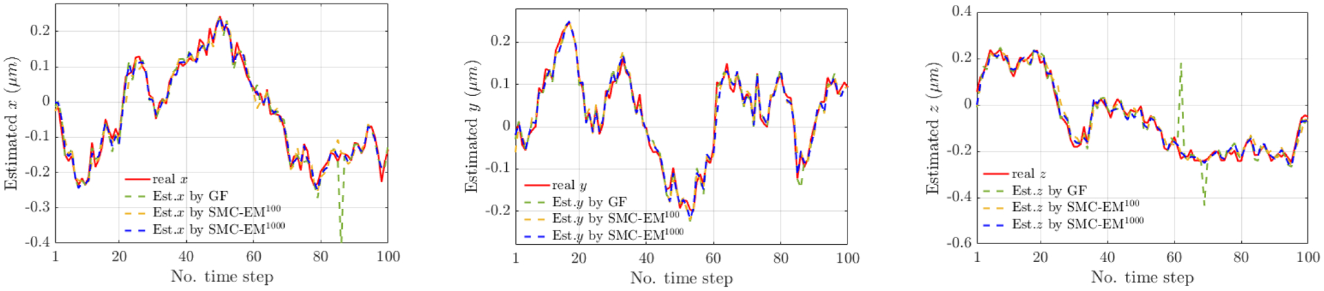
Typical simulation run of a particle confined to a cube with 500 nm sides centered at the origin. Each plot shows the (red, solid) true trajectory, (green dashed) GF estimate, and mean of the posterior distribution on the particle location using SMC-EM with (yellow dashed) 100 and (blue dashed) 1000 Monte Carlo samples.

4.2. Performance Demonstration

The localization performance (mean and standard deviation of RMSE) over the 20 trials is summarized in Table 2. And the corresponding boxplot of RMSE are shown in Fig. 4.

Table 2.

Summary of localization performance.

Method	RMSEx (nm)	RMSEy (nm)	RMSEz (nm)
GF-MLE	18.6773 ± 4.6255	14.5243 ± 1.3312	35.4456 ± 17.3784
SMC-EM100	19.9838 ± 1.1777	16.3672 ± 1.6846	25.4636 ± 3.3354
SMC-EM500	16.5215 ± 1.2763	14.2527 ± 1.0118	20.0875 ± 2.0706
SMC-EM1000	16.3922 ± 0.7239	14.0523 ± 1.0929	19.7188 ± 1.7344

Fig. 4.

Box plots of the RMSE where the solid line inside the box denotes the median, the box edges represent the first and third quartiles, the whiskers indicate the bounds for data within 1.5 times the interquartile range, and the red + symbols are outliers. Results are obtained by (black) GF-MLE, (green) SMC-EM¹⁰⁰, (blue) SMC-EM⁵⁰⁰, and (red) SMC-EM¹⁰⁰⁰.

As expected, the performance of SMC-EM improved with increasing MC samples. Except at the fewest number of MC samples, SMC-EM outperformed GF-MLE in localization, showing both lower error and smaller range in the estimates. Unlike GF, the use of the SMC-EM yielded similar accuracy in all three directions.

The results of estimation of the confinement lengths and diffusion coefficients are summarized in Table 3. In general, SMC-EM outperforms GF-MLE. Corresponding to the localization performance, the estimation of the diffusion coefficient as well as the confinement length gets improved with increasing number of MC samples.

Table 3.

Mean and standard deviation of of parameter estimation.

Method	Est.Dx (μm2/s)	Est.Dy (μm2/s)	Est.Dz (μm2/s)	Est.Lx (μm)	Est.Ly (μm)	Est.Lz (μm)
GF-MLE	0.0093 ± 0.0022	0.0083 ± 0.0017	0.0115 ± 0.0081	0.5342 ± 0.0740	0.5008 ± 0.0172	0.7454 ± 0.3189
SMC-EM100	0.0090 ± 0.0021	0.0094 ± 0.0018	0.0084 ± 0.0019	0.4866 ± 0.1145	0.4889 ± 0.1151	0.4376 ± 0.1030
SMC-EM500	0.0091 ± 0.0020	0.0093 ± 0.0016	0.0089 ± 0.0017	0.4736 ± 0.1115	0.4824 ± 0.1136	0.4416 ± 0.1039
SMC-EM1000	0.0092 ± 0.0017	0.0094 ± 0.0016	0.0093 ± 0.0013	0.5038 ± 0.0146	0.4964 ± 0.0165	0.5090 ± 0.0243

5. CONCLUSION

This paper built upon our prior work on bringing system identification tools to bear in estimation problems in SPT, extending it to include recent advances in observing three-dimensional trajectories based on the engineered DH-PSF and simplifying the computational complexity through the use of the aGPF and BSPS. Simulation results support the efficacy of the approach and show better performance than the current technique in the SPT community based on first estimating the particle trajectory using a GF and then determining model parameters based on MLE.

REFERENCES

- Anthony SM and Granick S (2009). Image analysis with rapid and accurate two-dimensional gaussian fitting. Langmuir, 25(14), 8152–8160. [DOI] [PubMed] [Google Scholar]
- Ashley TT and Andersson SB (2015). Method for simultaneous localization and parameter estimation in particle tracking experiments. Phys Rev E, 92(5), 052707. [DOI] [PubMed] [Google Scholar]
- Berglund AJ (2010). Statistics of camera-based single-particle tracking. Phys Rev E, 82(1), 011917. [DOI] [PubMed] [Google Scholar]
- Calderon CP (2016). Motion blur filtering: A statistical approach for extracting confinement forces and diffusivity from a single blurred trajectory. Phys Rev E, 93(5), 053303. [DOI] [PubMed] [Google Scholar]
- Chenouard N, Smal I, De Chaumont F, Maška M, Sbalzarini IF, Gong Y, Cardinale J, Carthel C, Coraluppi S, Winter M, et al. (2014). Objective comparison of particle tracking methods. Nat Methods, 11(3), 281. [DOI] [PMC free article] [PubMed] [Google Scholar]
- Dempster AP, Laird NM, and Rubin DB (1977). Maximum likelihood from incomplete data via the EM algorithm. J R Stat Soc Series B Stat Methodol, 39(1). [Google Scholar]
- Douc R, Garivier A, Moulines E, Olsson J, et al. (2011). Sequential Monte Carlo smoothing for general state space hidden Markov models. Ann Appl Probab, 21(6), 2109–2145. [Google Scholar]
- Doucet A, Godsill S, and Andrieu C (2000). On sequential monte carlo sampling methods for bayesian filtering. Statistics and Computing, 10(3), 197–208. [Google Scholar]
- Gu M (2000). Advanced Optical Imaging Theory. Springer. [Google Scholar]
- Handschin JE and Mayne DQ (1969). Monte carlo techniques to estimate the conditional expectation in multi-stage non-linear filtering. Int J Control, 9(5), 547–559. [Google Scholar]
- Hilzenrat G, Pandžić E, Yang Z, Nieves DJ, Goyette J, Rossy J, Ma Y, and Gaus K (2020). Conformational States Control Lck Switching between Free and Confined Diffusion Modes in T Cells. Biophys J, 118(6), 1489–1501. [DOI] [PMC free article] [PubMed] [Google Scholar]
- Jaeger JC and Carslaw HS (1959). Conduction of heat in solids. Clarendon P. [Google Scholar]
- Kotecha JH and Djuric PM (2003). Gaussian particle filtering. IEEE Trans Image Process, 51(10), 2592–2601. [Google Scholar]
- Kusumi A, Sako Y, and Yamamoto M (1993). Confined lateral diffusion of membrane receptors as studied by single particle tracking (nanovid microscopy). effects of calcium-induced differentiation in cultured epithelial cells. Biophysical journal, 65(5), 2021–2040. [DOI] [PMC free article] [PubMed] [Google Scholar]
- Lin Y and Andersson SB (2019). Simultaneous localization and parameter estimation for single particle tracking via sigma points based em. In 2019 IEEE 58th Conference on Decision and Control (CDC). [DOI] [PMC free article] [PubMed] [Google Scholar]
- Lin Y and Andersson SB (2021). Computationally efficient application of sequential monte carlo expectation maximization to confined single particle tracking. In 2021 European Control Conference (ECC). [DOI] [PMC free article] [PubMed] [Google Scholar]
- Michalet X and Berglund AJ (2012). Optimal diffusion coefficient estimation in single-particle tracking. Phys Rev E, 85(6), 061916. [DOI] [PMC free article] [PubMed] [Google Scholar]
- [Online] (2020). Movie of 3D single particle tracking using double-helix point spread function. https://drive.google.com/file/d/1K6b0sl5zq0p3fNsn5qpG7IkIF3fepVnH/view?usp=sharing. Accessed:2020-12-05.
- Pavani SRP, Thompson MA, Biteen JS, Lord SJ, Liu N, Twieg RJ, Piestun R, and Moerner W (2009). Three-dimensional, single-molecule fluorescence imaging beyond the diffraction limit by using a double-helix point spread function. Proc Natl Acad Sci USA. [DOI] [PMC free article] [PubMed] [Google Scholar]
- Särkkä S (2013). Bayesian filtering and smoothing, volume 3. Cambridge University Press. [Google Scholar]
- Schön T, Wills A, and Ninness B (2011). System identification of nonlinear state-space models. Automatica, 47(1), 39–49. [Google Scholar]
- Schütz GJ, Schindler H, and Schmidt T (1997). Single-molecule microscopy on model membranes reveals anomalous diffusion. Biophys J, 73(2), 1073–1080. [DOI] [PMC free article] [PubMed] [Google Scholar]
- Shen H, Tauzin LJ, Baiyasi R, Wang W, Moringo N, Shuang B, and Landes CF (2017). Single particle tracking: from theory to biophysical applications. Chem Rev, 117(11), 7331–7376. [DOI] [PubMed] [Google Scholar]
- Tanizaki H (2003). Nonlinear and non-gaussian state-space modeling with monte carlo techniques: A survey and comparative study. Handbook of Statistics, 21. [Google Scholar]