Abstract
Chimp optimization algorithm (ChOA) is a robust nature-inspired technique, which was recently proposed for addressing real-world challenging engineering problems. Due to the novelty of the ChOA, there is room for its improvement. Recognition and classification of marine mammals using artificial neural networks (ANNs) are high-dimensional challenging problems. In order to address this problem, this paper proposed the using of ChOA as ANN’s trainer. However, evolving ANNs using metaheuristic algorithms suffers from high complexity and processing time. In order to address this shortcoming, this paper proposes the fuzzy logic to adjust the ChOA’s control parameters (Fuzzy-ChOA) for tuning the relationship between exploration and exploitation phases. In this regard, we collect underwater marine mammals sounds and then produce an experimental dataset. After pre-processing and feature extraction, the ANN is used as a classifier. Besides, for having a fair comparison, we used a benchmark audio database of marine mammals. The comparison algorithms include ChOA, coronavirus optimization algorithm, harris hawks optimization, black widow optimization algorithm, Kalman filter benchmark algorithms, and also comparative benchmarks include convergence speed, local optimal avoidance ability, classification rate, and receiver operating characteristics (ROC). The simulation results show that the proposed fuzzy model can tune the boundary between the exploration and extraction phases. The convergence curve and ROC confirm that the convergence rate and performance of the designed recognizer are better than benchmark algorithms.
Keywords: Fuzzy system, Chimp optimization algorithm, Classification, Neural network. Marine mammals
Introduction
Recently, the processing of underwater audio signals in automatic recognition and classification of marine mammals has been expanding internationally and has become one of the favorite fields of researchers active in this field [9]. In other words, underwater sound signal processing is the newest way to measure the existence, abundance, and patterns of migratory marine mammals [5, 38].
The use of human-based methods and intelligent methods is one method of recognizing marine mammals. Initially, human operator-based methods were used to identify marine mammals. Its advantages include simplicity and ease of work [32]. However, the main disadvantage is the dependence on the operator’s psychological state and inefficiency in environments where the signal-to-noise ratio is low [22]. Then, contour-based recognition was used to recognition marine mammals due to their time complexity and low identification rate [13, 14]. To eliminate these defects, automatic target recognition (ATR) based on intelligent systems is used [3].
MLP-NN neural network, due to its simple structure, high performance, and low computational complexity, has become a useful tool for automatically recognizing targets [35]. In the past, MLP-NN training used gradient-based methods and error propagation, but these algorithms had a low convergence speed and were stuck in local minima [15, 25].
In recent years, we have witnessed the increasing use of meta-heuristic algorithms for the subject of neural network training. Genetic Algorithm (GA) [24], Simulated Annealing (SA) [20], Biogeography Algorithm (BBO) [28], Gray Wolf Optimizer (GWO) [10], Spider Community Algorithm (SSA) [27], Dragonfly Algorithm (DA) (Mohammad [19] and Algorithm for Finding No Progress (IWT) (M. [16] Suggested examples of the algorithm Existing meta-innovations that have been used as artificial neural network trainers. GA and SA are likely to reduce local optimization but converge at a slower rate. This works poorly in applications that require real-time processing. BBO has time-consuming calculations. GWO and IWT, despite their low complexity and high convergence speed, fall into the trap of local optimization, so they are not suitable for problems with local optimization. Many regulatory parameters and high complexity in the SSA algorithm are among the weaknesses of this algorithm. In addition to having many control parameters, DA has time-consuming calculations that are not suitable for real-time use.
The main reason for getting stuck in local optimizations is the imbalance between the two phases of exploration and extraction. Techniques for avoiding local optimization and creating trade-offs between the exploration and extraction phases include optimization with Chaotic maps [21], the use of non-linear coefficients [18], and utilize spiral shapes to improve performance [16] and linear control strategy (LCS) and arcsine-based non-linear control strategy (NCS-arcsine) [37]. On the other hand, the No Free Launch (NFL) theorem logically states that meta-heuristic algorithms do not have the same answer in dealing with different problems [33]. According to the NFL theory in this paper, a fuzzy system is used to create a triad between the exploration and extraction phases for MLP-NN training. The proposed technique for optimizing ChOA using a fuzzy system is called Fuzzy-ChOA, and in this article is indicated by the symbol FChOA.
In the following, the article is organized so that in part 2, it designs an experiment for data collection. Section 3 deals with the pre-processing of the obtained data and feature extraction. Section 4 discusses how to design an FChOA-MLPNN to automatically detect the sound produced by marine mammals. Section 5 will simulate and discuss it, and finally, Sect. 6 will conclude.
The experiment design and data acquisition
to obtain a real data set of sound produced by dolphins and whales from a research ship called the Persian Gulf Explorer and a Sonobuoy, a UDAQ_Lite data acquisition board, and three hydrophones (Model B& k 8013) were obtained was used with equal distance to increase the dynamic range. This test was performed in Bushehr port.
The raw data including 125 samples of Bottlenose Dolphin (10 sightings), 150 samples of Common Dolphin (18 sightings), 190 cases of Atlantic Spotted Dolphin (15 sightings), 106 cases of Sperm Whale (6 sightings), 115 samples of Northern Right Whale (10 sightings), and 172 samples of Killer Whale (8 sightings).
The ambient noise reduction and reverberation suppression
For example, the sounds emitted by marine mammals (dolphins and whales) recorded by the hydrophone array are considered x (t), y (t), z (t), and the original sound of dolphins and whales is considered s (t). The mathematical model of the output of hydrophones is in Eq. 1.
| 1 |
In Eq. 1, the Environment Response Functions (ERF) are denoted by h (t), g (t), and q (t). ERFs are unknown, and "tail" is considered uncorrelated [4], and naturally, the first frame of sound produced by marine mammals does not reach the hydrophone array at one time. Due to the sound pressure level (SPL) in the Hydrophone B&K 8103 and the reference (Hi and Testa n.d.), which deals with the underwater audio standard, the recorded sounds must be pre-amplified by factor.
Then, the Hamming window and Fast Fourier Transform (FFT) are applied to the frequency domain SPL. Next, frequency bandwidth is alleviated to 1 Hz bandwidth by Eq. 2.
| 2 |
SPLm is the obtained SPL at each fundamental frequency center in dB; re 1 μPa, SPL1 reduces SPL to 1 Hz bandwidth in dB; re one μPa, and Δf represents the bandwidth for each 1/3 Octave band filter. Wiener filter has been used to minimize the square mean error (MSE) between ambient noise and marine mammal noise [8]. After that, the results were calculated using Eqs. 3 to detect sounds with low SNR, i. e., less than 3 dB, deleted from the database.
| 3 |
where T, V, and A represent all the available signal, sound, and ambient sound, respectively. After that, the SPLs were recalculating at a standard measuring distance of 1 m as Eq. 4 (Fig. 1).
| 4 |
Fig. 1.
The ambient noise reduction and reverberation suppression block diagram
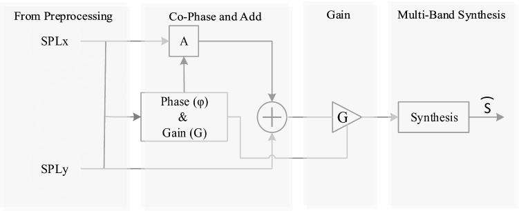
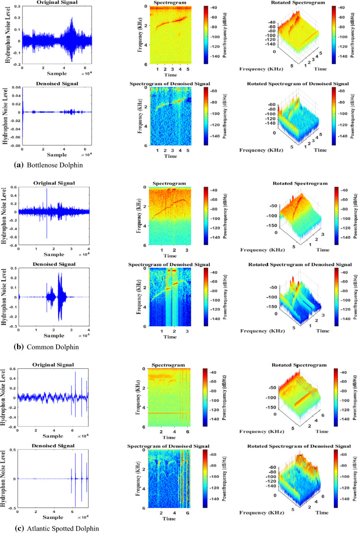
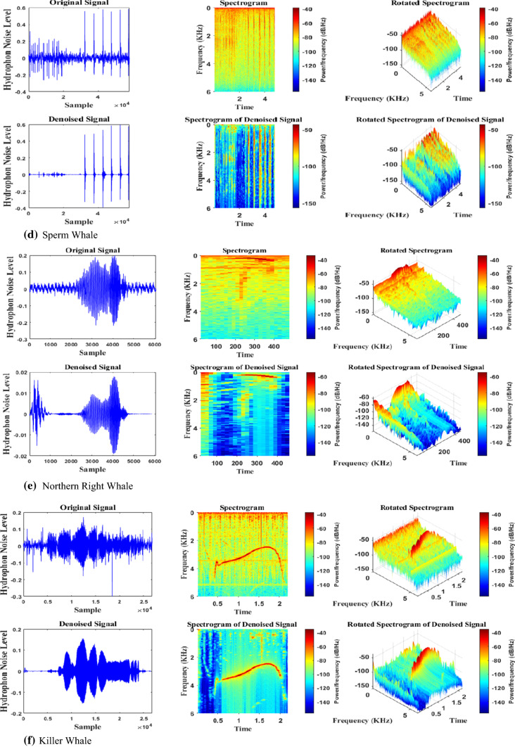
In the next part, the effect of reverberation must be removed. In this regard, the common phase is added to the band (reducing the phase change process using the delay between the cohesive parts or the initial sound is called the common phase) [29]. Therefore, a cross-correlation pass function by adjusting each frequency band’s gain eliminates non-correlated signals and passes the correlated signals. Finally, in each frequency band, the output signals are combined to generate the estimated signal, i. e. . The reverberation removal block diagram is indicated in Fig. 2. Typical representations for dolphin and whale sounds and melodies and their spectroscopy are shown in Fig. 3.
Fig. 2.
The block diagram of the reverberation removal section
Fig. 3.
Typical sound presentations produced by dolphins and whales and their spectrogram
It must be noted that the application of the gain controller depends on different inputs. For example when x and y are the same, i.e. , or one of them is delayed by a few milliseconds, the delay is adjusted automatically as , where T is a hypothetical delay modification. If the delay is greater than the window length L, the x and y are being uncorrelated and the gain is being zero. Finally, when x and y are uncorrelated, totally, is zero.
All of the terms are true for each frequency band. Thus if x and y are uncorrelated at one frequency and correlated at another, then the uncorrelated part is removed and the correlated part remains. Since all of the operations are defined on a moving average basis, everything may change as a function of time.
average cepstral features and cepstral liftering features.
The effect of ambient noise and reverberation decreases after detecting the audio signal frames obtained in the pre-processing stage. In the next step, the detected signal frames enter the feature extraction stage. The sounds made by dolphins and whales emitted from a distance to the hydrophone experience changes in size, phase, and density. Due to the time-varying multipath effect, fluctuating channel complicates the dolphins and whales recognition task. The cepstral factors with the cepstral liftering feature can significantly alleviate the multipath effects, while the average cepstral coefficients can notably eliminate the time-varying effects of shallow underwater channels [6]. Therefore, this section proposes the use of cepstral features, including mean cepstral features and cepstral liftering features, to make a valid data set. The channel response cepstrum and the original sound dolphins and whales cepstrum could be separated by higher and lower cepstrum indices, respectively [5]. They are in non-overlapping parts of the liftering cepstrum. Thus, the quality of the features is improved by lower time liftering. After the noise and reverberation removal, the frequency domain frames of SPLs (S(k)) are transferred to the cepstrum feature extraction section. The following Equation calculates the cepstrum features of the sound generated with dolphins and whale's signals.
| 5 |
where S(k) represents the frequency domain frames of sounds generate dolphins and whales SPLs, N denotes the number of discrete frequencies used for FFT, Hl (k) shows the transfer function of the Mel-scaled triangular filter, where l = 0, 1,…, M. Finally, cepstral coefficients are transferred back to the time domain as c(n) by Discrete Cosine Transform (DCT).
As mentioned earlier, the sound produced by dolphins and whales is extracted by Low-time liftering process. Thus, the low-time liftering is proposed as Eq. 6 to extract the sound that originated from the whole sound.
| 6 |
Lc shows the length of the liftering window, which is used as 15 or 20. The final features can be calculated by multiplying the cepstrum c(n) with the and applying logarithm and DFT functions as Eqs. 7 and 8, respectively.
| 7 |
| 8 |
Finally, the feature vector would be represented using Eq. 9.
| 9 |
The first 512-cepstrum points (out of 8192 points in one frame for a sampling rate of 8192 Hz, except for zeroth index {}) are corresponded to 62.5 ms liftering coefficients, are windowed from the N indices, which is equivalent to one frame length to reduce the liftering coefficients to 44 features. The length of sub-frames, before averaging, is five seconds. During the averaging liftering process, ten previous frames comprise 50 s average cepstral features. The final average cepstral features are calculated by smoothing those ten frames. Consequently, the average cepstral feature vector consists of 44 features. In the next phase, the Xm vector would be an input vector for an MLP-NN.
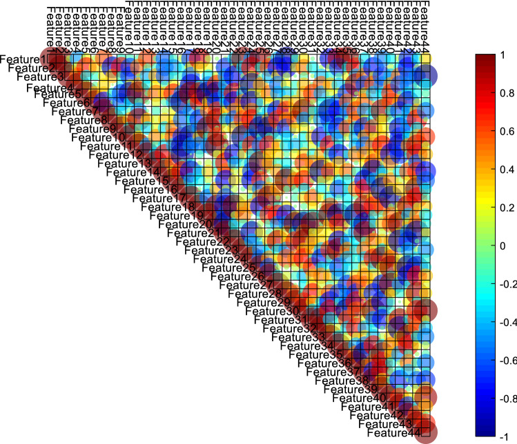
To sum up, the number of neural network inputs is equal to P. The whole process of the feature extraction stage is indicated in Fig. 4. To sum up, the output of this stage is shown in Fig. 5.
Fig. 4.
The block diagram of the cepstrum liftering feature extraction process
Fig. 5.
Correlation matrix for extracted features
The correlation matrix shows the correlation coefficients between the variables (or features). Each cell in the table shows the correlation between the two variables. Correlation between two variables means measuring the prediction of values of one based on the other. This means that the higher the correlation coefficient, the greater the possibility of predicting the value of one variable over the other. Pearson and Spearman correlation coefficients are between 1 and − 1. Thus, if the correlation coefficient is close to or equal to 1, there is a strong correlation between the two variables. In this case, we can say that the direction of change of both variables is similar to each other.
As shown in Fig. 5, the extracted features are not highly correlated with each other. Therefore, relatively good features have been extracted (Fig. 6).
Fig. 6.
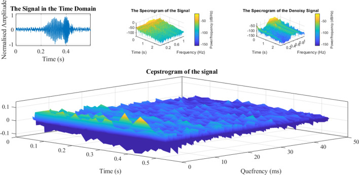
The typical visualization of produce sound cepstrum features (Northern Right Whale)
Design of an FChOA-MLPNN for automatic detection of sound produced by marine mammals
MLP-NN is the simplest and most widely used neural network [23]. Important applications of MLP-NN include automatic target recognition systems. For this reason, this article uses MLP-NN as an identifier [2]. MLP-NN is one of the most robust neural networks used for systems with high nonlinearity. Also, the MLP-NN is a feed-forward network capable of non-linear fittings with higher precision. Despite what has been said, one of the challenges facing MLP-NN is always training and adjusting the edges' bias and weight [7].
The steps for using meta-heuristic algorithms to teach MLPNN are as follows: The first phase determines how to display the connection weights. The second phase assesses the fitness function to evaluate these connection weights, which can be considered Mean Square Error (MSE) for the recognition problems. In the third phase, the evolutionary process is used to minimize the fitness function, which is the MSE.
The technical design of the evolutionary strategy of connection weights training can be presented in Fig. 7 and Eq. 10.
| 10 |
where i represents the number of the input nodes, h denotes the number of the hidden nodes, indicates the connection weight from the ith input node to the hth hidden node, denotes the bias (threshold) of the hth hidden neuron, indicates the connection weight from the hth hidden node to the mth output node.
Fig. 7.
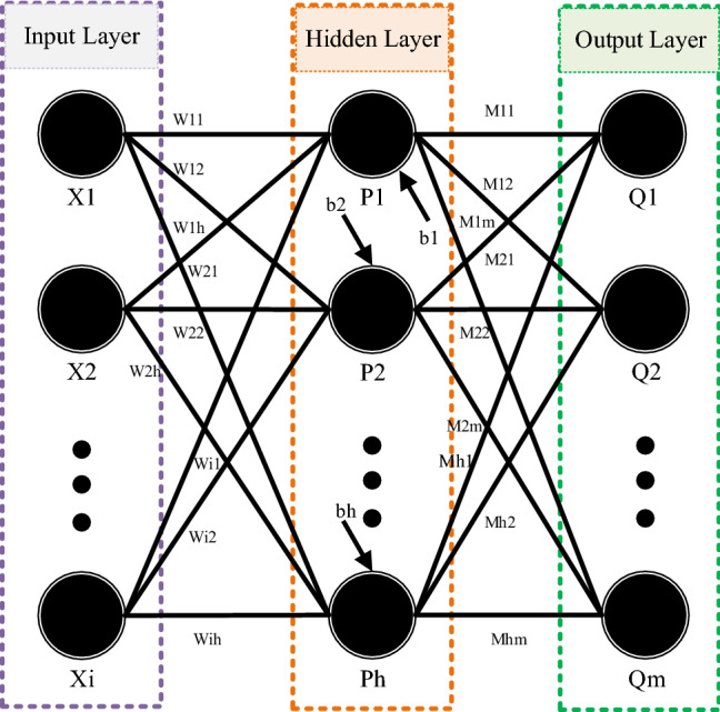
Introduction of MLP-NN as a search agent for a meta-heuristic algorithm
As previously stated, the MSE is a common criterion for evaluating an MLP-NNs as Eq. 11.
| 11 |
where m is the number of neurons in the MLP outputs, is the optimal output of input unit in cases where training sample is utilized, and denotes the real output of input unit in cases where the training sample is observed in the input. The MLP must be adapted to a set of training samples to be effective. Therefore, MLP performance based on the mean MSE on all training samples is calculated as:
| 12 |
T denotes the number of training samples, denotes the optimal output related to ith input when using kth the training sample, and m denotes the number of outputs and indicates the input’s real output when using the training sample. In the final stage, the recognizer needs a meta-heuristic algorithm to tune the parameters mentioned above. The next section proposes using an enhanced chimp optimization algorithm (ChOA) with fuzzy logic called FChOA as an instructor.
Fuzzy-ChOA
In this section, a fuzzy system is proposed as a ChOA developer. The first subsection introduces the ChOA algorithm, and the second subsection describes how to use the fuzzy system to adjust the ChOA control parameters.
Chimp optimization algorithm
This algorithm was introduced in 2020, inspired by the way chimps were hunted by Khishe and Mousavi ([17]. The behavior of the first two roles in team hunting, driver and chase, is statistically described next:
| 13 |
| 14 |
t represents the number of current iterations, a, m, and c are coefficient vectors, is the prey position vector, and is the Chimp position vector. The vectors a, m and c, are calculated by Eqs. (15), (16), and (17), respectively.
| 15 |
| 16 |
| 17 |
where f decreases nonlinearly by the iteration process from 2.5 to zero (in both exploration and extraction stages), while and are random vectors in the interval [1,0]. Also, m is a vector that is calculated based on turbulent maps. This vector indicates the effect of Chimp's sexual motivation on the hunting process.
The stochastic population generation of chimps is the first step in the ChOA algorithm. Next, the chimps are randomly arranged into four independent groups: driver, barrier, chaser, and attacker. Each group strategy will determine the location updating method of individual chimps by determining the f vector, while all of the groups aim to estimate the potential prey’s positions. The c and m vectors are tuned adaptively and will enhance the local minima avoidance and convergence rate.
Chimps (driver, barrier, and chaser) search for prey and then surround it. The hunting process is usually carried out by invading chimps. Chasing stimuli, obstacles, and Chimps sometimes participate in the hunting process. To mathematically simulate chimps' behavior, it is assumed that the first attacker (the best solution available), the stimulus, the obstacle, and the pursuer are more aware of the potential prey's location. Thus, the four solutions that are the best solution are obtained, stored, and the other Chimps are forced to update their positions according to the best Chimp locations. This relationship is expressed by Eqs. (18), (19), and (20).
| 18 |
| 19 |
| 20 |
The m parameter mathematically models chimps' chaotic behavior in the hunt's final stage to obtain more meat and, subsequently, more social favors such as grooming.
Proposed fuzzy controlled system to adjust ChOA control parameters
All optimization algorithms have essential and influential parameters [30]. These parameters play a significant role in the search process. For example, early convergence, convergence rate, local optimization, exploration, and extraction depend on the correct and dynamic adjustment of these significant parameters. As shown in the previous section and Eqs. (15) and (16), a and c are two critical parameters in ChOA. On the other hand, parameters a and c in classical ChOA are influenced by random components and . In references ([31], fuzzy inference has been used as an automatic adjuster of control parameters to upgrade and modify them. According to studies, the fuzzy system is a suitable candidate for intelligent control of control parameters. It should be noted that efficiency and complexity in most intelligent systems based on meta-heuristic algorithms are directly related. The higher the efficiency, the more complex the parallel. Therefore, the use of an additional intelligent controller (fuzzy controller) increases the computation's complexity, which improves the performance of the high-dimensional feature space. Therefore, this paper uses fuzzy inference to develop ChOA.
The proposed fuzzy system has three stages of fuzzyization, fuzzy inference, and de-fuzzy. The first step is fuzzy construction. This step converts the inputs to the fuzzy model for processing based on a fuzzy system. In the second step, the fuzzy system evaluates and infers the rules using the Mamdani inference algorithm. The last step is called defuzzification, in which the results of fuzzy inference, which are in the form of fuzzy sets, are converted into quantitative data and information.
Fig. 8. shows the proposed fuzzy model for adjusting the control parameters of the chimp optimization algorithm.
Fig. 8.
A proposed fuzzy model for setting parameters a and c
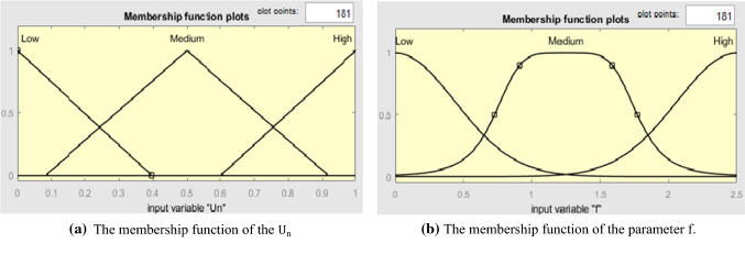
In this model, the membership functions for fuzzification (shown in Fig. 9) are:
Fig. 9.
the membership functions for fuzzification
: The number of repetitions in which the fitness function has not changed. The the membership function is shown in Fig. 9(a).
The parameter f: f is reduced nonlinearly from the range of 2.5 to zero by the iteration process. Any continuous function can perform independent group updates. These functions must be selected so that f decreases during each iteration. The membership function f is shown in Fig. 9(b).
After fuzzification of input data, a set of rules is presented using the Mamdani algorithm according to Table 1. Next, the Mamdani inference machine's output will be defuzzification by two membership functions of parameters a and c. The de-fuzzy phase consists of two parameters, a and c, which, if properly adjusted, will define the boundary between the exploration and extraction phases. Defuzzification membership functions (shown in Fig. 10) The two parameters a and c are:
Table 1.
Fuzzy rules used
| Rules |
|---|
| If (Un is Low) and (f is Low), Then (a is Medium_High) and (c is Medium) |
| If (Un is Low) and (f is Medium), Then (a is Medium_Low) and (c is Medium_Low) |
| If (Un is Low) and (f is High), Then (a is High) and (c is Low) |
| If (Un is Medium) and (f is Low), Then (a is Medium_High) and (c is Medium_High) |
| If (Un is Medium) and (f is Medium), Then (a is Medium_High) and (c is Medium_Low) |
| If (Un is Medium) and (f is High), Then (a is Medium_High) and (c is Low) |
| If (Un is High) and (f is Low), Then (a is Medium) and (c is High) |
| If (Un is High) and (f is Medium), Then (a is Medium_Low) and (c is Medium_Low) |
| If (Un is High) and (f is High), Then (a is High) and (c is Low) |
Fig.10.
the membership functions for defuzzification
The parameter a: a is a random variable in the range [5, − 5]. This parameter leads to convergence or divergence of search agents to prey. Figure 10.a shows the membership function of parameter a.
The c: c parameter is a random variable in the range [2 and 0]. Vector c always needs to generate random values and execute the exploration process in the initial iterations and the final iterations. This factor has been beneficial to avoid the occurrence of local minimum points. Figure 10(b) shows the membership function of parameter a.
Simulation results and discussion
to show the power and efficiency of MLP-FChOA, in addition to using the sounds obtained in Sects. 2 and 3, the reference dataset [36] is also used. As already mentioned, To obtain the data set, the vector is assumed to be an input for the MLP-FChOA. The dimension is 645 , which implies that the data set contains 44 features and 645 samples. Also, the dimension of the benchmark dataset is 435 .
In MLP-FChOA, the number of input nodes is equal to the number of features. 70% of the data was used for training, and 30% was used for testing. To have a fair comparison between the algorithms, the condition of stopping 300 iterations is considered. There is no specific equation for obtaining the number of hidden layer neurons, so Eq. 23 is used to obtain it [26].
| 23 |
where N shows the number of the inputs, and H denotes the number of the hidden nodes. Similarly, the number of output neurons is equivalent to the marine mammal classes, i. e., six neurons.
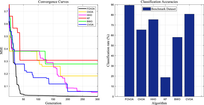
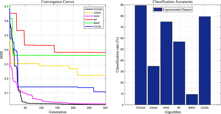
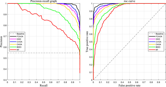
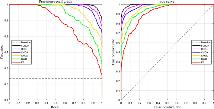
In order to have a fair evaluation of FChOA, the performance of this algorithm with five benchmark algorithms ChOA (M. [17], CVOA[34], HHO [12], KF [1], and BWO [11] are measured. The basic parameters and the primary values of these benchmark algorithms get demonstrated in Table 2. The classifiers' performance is then tested for classification rate, local minimum avoidance, and convergence speed. Each algorithm is run 33 times, and the classification rate, mean and standard deviation of the minimum error, and P-value are shown in Table 3. Mean values and standard deviation of minimum error and P-value indicate the algorithm's strength in avoiding local optimization. Figures 11 and 13 also show a comprehensive comparison of the convergence speed and syntax and the classifiers' final error rate. Figures 12 and 14 show the ROC curve to demonstrate the ability to evaluate classifiers. All of the evaluation was carried out in MATLAB-R2020a, on a PC with processor Intel Core i7-4500u with a 2.3 GHz processor, 5 GB RAM running memory, in Windows 10.
Table 2.
The initial parameters and primary values of the benchmark algorithms
| Algorithm | Parameter | Value |
|---|---|---|
| ChOA | Random values | |
| m | Chaotic maps | |
| Number of chimps | 55 | |
| FChOA | Tuning using a fuzzy system | |
| m | Chaotic maps | |
| Number of chimps | 55 | |
| CVOA | P-die | 0.06 |
| P_isolation | 0.7 | |
| P_Superspreader | 0.2 | |
| P_reinfection | 0.03 | |
| Social_distancing | 9 | |
| P_Travel | 0.2 | |
| Pandemic_duration | 31 | |
| BWO | PP | 0.7 |
| CR | 0.45 | |
| PM | 0.5 | |
| HHO | v,u | Random values inside (0,1) |
| B | Constant set to 1.5 | |
| KF | The covariance matrix of state estimation error | R = 40I |
| Covariance matrix of artificial Noise | Q = 40I | |
| Covariance matrix of artificial Noise | PO = 40I |
Table 3.
Results were obtained from different algorithms
| Training method | MLP training algorithms | Benchmark dataset | Experimental dataset | ||||
|---|---|---|---|---|---|---|---|
| MSE(AVE±STD) | P-value | Classification rate % | MSE(AVE ± STD) | P-value | Classification rate % | ||
| ChOA | 0.1381 ± 0.1483 | 1.351 | 65.6015 | 0.1388 ± 0.1563 | 2.009 | 35.8461 | |
| Metahsoristic | FChOA | 0.1016 ± 0.1121 | 0.038 | 89.3480 | 0.1006 ± 0.1222 | 0.019 | 89.1355 |
| CVOA | 0.1277 ± 0.1371 | 0.184 | 81.9422 | 0.1254 ± 0.1451 | 0.106 | 79.0043 | |
| BWO | 0.1421 ± 0.1509 | 2.169 | 58.0248 | 0.1254 ± 0.1451 | 2.894 | 58.8453 | |
| HHO | 0.1109 ± 0.1295 | 0.086 | 76.1208 | 0.1192 ± 0.1386 | 0.057 | 74.0199 | |
| KF | 0.1611 ± 0.1662 | 2.871 | 18.01533 | 0.1530 ± 0.17244 | 3.322 | 57.9411 | |
| Traditional | GD | 0.5944 ± 0.6231 | 6.7892 | 13.4590 | 0.69908 ± 0.2576 | 6.908 | 11.9184 |
Fig. 11.
Convergence diagram of different training algorithms for benchmark dataset
Fig. 13.
Convergence diagram of different training algorithms for Datasets obtained in parts 2 and 3
Fig. 12.
The ROC curves and precision-recall curves for different training algorithms for benchmark dataset
Fig. 14.
The ROC curves and precision-recall curves for different training algorithms for datasets are obtained in parts 2 and 3
Figures 10, 11, 12, 13, 14 show the simulation results of MLP training using different metaheuristic algorithms. For a more comprehensive study and a fairer comparison, in Table 3, in addition to the simulation results of MLP training using metaheuristic methods, the simulation results using the traditional method of descent gradient (GD) are also discussed. Considering the values obtained in the measured metrics, the use of GD for MLP training in this investigation is very disappointing.
Adding a subsystem to a metaheuristic algorithm increases its complexity. However, a comparison of the convergence curves in Figs. 11 and 13 shows that the FChOA achieved the global optimum faster than the other algorithms used. Other algorithms were stuck in the local optimum if they converged. In particular, by comparing the ChOA and FChOA in Fig. 13, it can be seen that the use of an auxiliary (fuzzy system) subsystem is necessary to avoid getting caught up in the local optimum in the ChOA. In general, using a fuzzy system to improve ChOA increases complexity. However, the convergence curves and better performance of FChOA than other algorithms used show a reduction in computational cost. Another evidence that, despite increasing complexity, shows an improvement in FChOA performance is the lower MSE of this algorithm compared to other algorithms used.
As shown in Figs. 11 and13, among the benchmark algorithms used for MLP training, FChOA has the highest convergence speed by correctly detecting the boundary between the exploration and extraction phases. KF has the lowest convergence speed by adjusting control parameters. As shown in Table 3, MLP-FChOA has the highest classification rate, and MLP-KF has the lowest classification rate among the classifiers. The STD values, shown in Table 3, indicate that the MLP-FChOA results rank first in the two datasets, confirming that the FChOA performs better than other standard training algorithms and demonstrates the FChOA's ability to avoid getting caught up in local optimism. A P-value of less than 0.05 indicates a significant difference between FChOA and other algorithms. As shown in Figs. 12 and 14, the ROC curve also confirms the algorithm’s better performance. Generally, the precision-recall plot shows the trade-off between recall and precision for various threshold levels. A high area under the precision-recall curve represents high precision and recall. High precision indicates a low false-positive rate, and high-recall indicates a low false-negative rate. As can be observed from the curves in Fig. 12, FChOA has a higher area under the precision-recall curves.
Conclusion
This paper classified marine mammals based on intelligent systems and used with an MLP-NN as a classifier. The neural training network was performed using ChOA, FChOA, CVOA, BWO, HHO, KF. The simulation results showed that the fuzzy system performs the task of adjusting and controlling the primary and proper parameters of FChOA well and makes the algorithm powerful in determining the boundary between the exploration and extraction phases and finding it possible to find the optimal global algorithm and avoid getting stuck and Prevents local optimizations. The convergence and ROC curves indicate MLP-FChOA, MLP-HHO, MLP-CVOA, MLP-ChOA, MLP-BWO, and MLP-KF, respectively, perform better in the classification of marine mammals based on the sound emitted from them, respectively. Also, the fastest convergence speed is related to the MLP-FChOA classifier.
The research topics for the future are as follows:
Using deep learning to classify marine mammals
Using of RBF network and metaheuristic algorithms to classify marine mammals
Investigating the role of chaotic maps in improving the training of ANNs using metaheuristic mammal
Implement FChOA to classify marine mammals using FPGA
Design of optimal neural network structure for marine mammal classification
Biographies
Abbas Saffari
was born in Touyserkan, Iran, in 1992. He received his B.Sc. degree in 2013 and M.Sc.degree in 2016 from Imam Khomeini Marine University, Department of Electrical Engineering. he is currently a Ph.D. candidate in Electronic Engineering at the University of Birjand. Research interests are Neural Networks, Meta-Heuristic Algorithm, video and image processing, Sonar, and Classification.
Mohammad Khishe
was born in 1985 in Nahavand, Iran. He received the B.Sc. degree in Maritime Electronics and Communication Engineering from Imam Khomeini Maritime Sciences University, Nowshahr, Iran in 2007 and also, M.Sc. and Ph.D. degrees in Electronic Engineering from Islamic Azad University, Qazvin branch and Iran University of Science and Technology, Tehran, in 2012 and 2017, respectively. Since 2011, he is a faculty member of Maritime Electrical and Electronic Engineering at Imam Khomeini Maritime Sciences University, Nowshahr, Iran. His research interests are Digital Signal Processing, Artificial Neural Networks, Meta-heuristic Algorithms, Sonar and Radar Signal Processing, and FPGA design.
Seyed-Hamid Zahiri
received the B.Sc., M.Sc., and Ph.D. degrees in Electronics Engineering from Sharif University of Technology, Tehran, Tarbiat Modarres University, Tehran, and Mashhad Ferdowsi University, Mashhad, Iran, in 1993, 1995, and 2005, respectively. He is currently a Professor with the Department of Electronics Engineering, University of Birjand, Birjand, Iran. His research interests include pattern recognition, evolutionary algorithms, swarm intelligence algorithms, and soft computing.
Footnotes
Publisher's Note
Springer Nature remains neutral with regard to jurisdictional claims in published maps and institutional affiliations.
References
- 1.Abdul A, et al. Engineering applications of artificial intelligence regulated kalman filter based training of an interval type-2 fuzzy system and its evaluation. Eng. Appl. Artif. Intell. 2020;95:103867. doi: 10.1016/j.engappai.2020.103867. [DOI] [Google Scholar]
- 2.Aitkin M, Foxall ROB. “Statistical modelling of artificial neural networks using the multi-layer perceptron. Statist. Comput. 2003;1(1):227–39. doi: 10.1023/A:1024218716736. [DOI] [Google Scholar]
- 3.Bhanu BIR. Automatic target recognition : state of the art survey. IEEE Trans. Aerosp. Electron. Syst. 1986;4:364–379. doi: 10.1109/TAES.1986.310772. [DOI] [Google Scholar]
- 4.Allen JB, Berkley DA, Blauert J. Multimicrophone signal-processing technique to remove room reverberation from speech signals. The Journal of the Acoustical Society of America. 1977;62:912. doi: 10.1121/1.381621. [DOI] [Google Scholar]
- 5.Das A, Kumar A, Bahl R. Radiated signal characteristics of marine vessels in the cepstral domain for shallow underwater. J. Acoust. Soc. Am. 2012;128(4):EL151–EL156. doi: 10.1121/1.3484230. [DOI] [PubMed] [Google Scholar]
- 6.Das A, Kumar A, Bahl R. Marine vessel classification based on passive sonar data : the cepstrum-based approach. IET Radar Sonar & Navig. 2013;7(1):87–93. doi: 10.1049/iet-rsn.2011.0142. [DOI] [Google Scholar]
- 7.D. Devikanniga, K. Vetrivel, and N. Badrinath, Review of meta-heuristic optimization based artificial neural networks and its applications. In Journal of Physics: Conference Series 1362(1) (2019)
- 8.Gallardo D, Sahni O, Bevilacqua R. Hammerstein —wiener based reduced—order model for vortex-induced non—linear fluid-structure interaction. Eng. Comput. 2016;33(2):219–37. doi: 10.1007/s00366-016-0467-9. [DOI] [Google Scholar]
- 9.González-hernández FR, Sánchez-fernández LP, Suárez-guerra S, Sánchez-pérez LA. Marine mammal sound classification based on a parallel recognition model and octave analysis. Appl. Acoust. 2017;119:17–28. doi: 10.1016/j.apacoust.2016.11.016. [DOI] [Google Scholar]
- 10.Hadavandi E, Mostafayi S, Soltani P. A grey Wolf optimizer-based neural network coupled with response surface method for modeling the strength of Siro-Spun Yarn in spinning mills. Appl. Soft Comput. J. 2018;72:1–13. doi: 10.1016/j.asoc.2018.07.055. [DOI] [Google Scholar]
- 11.Hayyolalam V, PourhajiKazem AA. Black widow optimization algorithm: a novel meta-heuristic approach for solving engineering optimization problems. Eng. Appl. Artif. Intell. 2020;87:103249. doi: 10.1016/j.engappai.2019.103249. [DOI] [Google Scholar]
- 12.Heidari AA, et al. Harris Hawks Optimization : algorithm and applications. Future Gener. Comput. Syst. 2019 doi: 10.1016/j.future.2019.02.028. [DOI] [Google Scholar]
- 13.Hi, H., et al. The specialist committee on hydrodynamic noise. Final Report and Recommendations to the 28th ITTC (Vol. 2, pp. 502–578).
- 14.Hurtado J, et al. Enveloping CAD models for visualization and interaction in XR applications. Eng. Comput. 2020 doi: 10.1007/s00366-020-01040-9. [DOI] [Google Scholar]
- 15.Keshtegar B. Limited conjugate gradient method for structural reliability analysis. Eng. Comput. 2016;33(3):621–629. doi: 10.1007/s00366-016-0493-7. [DOI] [Google Scholar]
- 16.Khishe M, Mosavi MR. Improved whale trainer for sonar datasets classification using neural network. Appl. Acoust. 2019;154:176–192. doi: 10.1016/j.apacoust.2019.05.006. [DOI] [Google Scholar]
- 17.Khishe M, Mosavi MR. Chimp optimization algorithm. Exp. Syst. Appl. 2020;149:113338. doi: 10.1016/j.eswa.2020.113338. [DOI] [Google Scholar]
- 18.M. Khishe, M.R. Mosavi, M. Kaveh, in The Fourth Iranian Conference on Engineering Electromagnetics Sonar Data Set Classification Using MLP Neural Network Trained by Non-Linear Migration Rates BBO (2016)
- 19.Khishe M, Safari A. Classification of sonar targets using an MLP neural network trained by Dragonfly algorithm. Wirel. Pers. Commun. 2019;108(4):2241–2260. doi: 10.1007/s11277-019-06520-w. [DOI] [Google Scholar]
- 20.Koh CS, Hahn SY. Detection of magnetic body using artificial neural network with modified simulated annealing. IEEE Trans. Magn. 1994;30(5):3644–3647. doi: 10.1109/20.312730. [DOI] [Google Scholar]
- 21.Lu H, Wang X, Fei Z, Qiu M. The effects of using Chaotic map on improving the performance of multiobjective evolutionary algorithms. Math. Prob. Eng. 2014 doi: 10.1155/2014/924652. [DOI] [Google Scholar]
- 22.F. Maire, L.M. Alvarez, A. Hodgson, Automating marine mammal detection in aerial images captured during wildlife surveys: a deep learning approach, in Lecture Notes in Computer Science (including subseries Lecture Notes in Artificial Intelligence and Lecture Notes in Bioinformatics) 9457: 379–85 (2015)
- 23.M.M. Mijwil, A. Alsaadi, Overview of neural networks (2019)
- 24.D.J. Montana, L. Davis, Training feedforward neural networks using genetic algorithms. In Proceedings of the 11th International Joint Conference on Artificial intelligence, vol 1 89: pp. 762–67. http://dl.acm.org/citation.cfm?id=1623755.1623876 (1989)
- 25.Moradi Z, Mehrvar M, Nazifi E. Genetic diversity and biological characterization of sugarcane streak mosaic virus isolates from Iran. VirusDisease. 2018;29(3):316–323. doi: 10.1007/s13337-018-0461-5. [DOI] [PMC free article] [PubMed] [Google Scholar]
- 26.Mosavi MK, Khishe M, Mosavi MR. Design and implementation of a neighborhood search biogeography- based optimization trainer for classifying sonar dataset using multi—layer perceptron neural network. Analog Integr Circuits Signal Process. 2018 doi: 10.1007/s10470-018-1366-3. [DOI] [Google Scholar]
- 27.Pereira, L., et al. (2014). Social-spider optimization-based artificial neural networks training and its applications for Parkinson’s disease identification. In Proceedings IEEE Symposium on Computer-Based Medical Systems (pp. 14–17).
- 28.Pu X, Chen S, Yu X, Zhang L. Developing a novel hybrid biogeography-based optimization algorithm for multilayer perceptron training under big data challenge. Sci. Prog. 2018 doi: 10.1155/2018/2943290. [DOI] [Google Scholar]
- 29.Bretschneider, H., et al. The specialist committee on hydrodynamic noise. Final Report and Recommendations to the 27th ITTC (pp. 639–690).
- 30.Rodr, L., Castillo, O., & Soria, J. (2017). A study of parameters of the grey wolf optimizer algorithm for dynamic adaptation with fuzzy logic. In Nature-inspired design of hybrid intelligent systems (pp. 371–390).
- 31.Rodriguez, L., et al. (2017). Dynamic simultaneous adaptation of parameters in the Grey Wolf optimizer using fuzzy logic. In 2017 IEEE International Conference on Fuzzy Systems (FUZZ-IEEE).
- 32.Shiu Yu, et al. Deep neural networks for automated detection of marine mammal species. Sci. Rep. 2020;10(1):1–12. doi: 10.1038/s41598-019-56847-4. [DOI] [PMC free article] [PubMed] [Google Scholar]
- 33.Simaan MA. Simple explanation of the no-free-lunch theorem and its implications. J. Optim. Theory Appl. 2003;115(3):549–70. [Google Scholar]
- 34.Martínez-Álvarez F, et al. Coronavirus optimization algorithm: a bioinspired metaheuristic based on the COVID-19 Propagation Model. Big Data. 2020;8(4):308–322. doi: 10.1089/big.2020.0051. [DOI] [PubMed] [Google Scholar]
- 35.Wang H, Moayedi H, Foong LK. Genetic algorithm hybridized with multilayer perceptron to have an economical slope stability design. Eng. Comput. 2020 doi: 10.1007/s00366-020-00957-5. [DOI] [Google Scholar]
- 36.W.A. Watkins et al. “W Lt ^ I.” (code 211): 4 (1992)
- 37.Wu X, Zhang SEN, Xiao W, Member S. The exploration / exploitation trade-off in whale optimization algorithm. IEEE Access. 2019;7:125919–125928. doi: 10.1109/ACCESS.2019.2938857. [DOI] [Google Scholar]
- 38.Lubis ZM, Mujahid M, Harahap MS, Tauhid M. Signal processing : passive acoustic in fisheries and marine mammals. J Biosens. Bioelectron. 2016;7(208):2. [Google Scholar]


