

Abstract
The current study was performed to develop dynamic quality and shelf-life prediction models using selected index for packaged chicken meat during storage. Generally, the results showed that meat deterioration, with respect to the different quality indices considered in the investigation, proceeds with increasing temperature and storage time. Highly significant (P ≤ 0.01) correlations were obtained between TPC (total plate count) and SI (sensory index) (r = −0.94 to −0.97), coliforms and SI (r = −0.89 to −0.95), and LAB (lactic acid bacteria) and SI (r = −0.93 to −0.98). However, only the microbiological spoilage regarding TPC, whose values ranged from 7.0 to 8.0 log CFU/g under all investigated temperature conditions, were in compliance with the end of sensory shelf-life defined at SI = 5. To develop dynamic quality prediction model, 4 isothermal (0, 4, 10, and 15°C) experiments in 2 batches were performed for TPC evaluation. Growth data were fitted in the Baranyi and Roberts and quadratic polynomial model as the primary and secondary models, respectively. The model was validated under dynamic conditions (0–8°C scenario with periodic 12-h changes). The accuracy and bias factors were estimated to be 1.045 and 0.991 for fluctuating conditions and 1.016 and 1.015 for real-time conditions, respectively, suggesting good applicability of the model. The remaining shelf-life estimation model developed based on mean kinetic temperature showed an even decrease of shelf-life under dynamic conditions in time. The developed model scan can be used for effective monitoring of packaged chicken meat freshness and shelf-life during distribution with temperature fluctuation.
Key words: chicken meat freshness, total plate count, sensory index, dynamic quality prediction model, mean kinetic temperature
INTRODUCTION
Consumption of chicken has recently increased widely all over the world (Grau et al., 2011; Ghollasi-Mood et al., 2016) due to its relatively low fat content, high nutritional value, and distinct flavor (Choe et al., 2010). Especially, the chicken breast meat is considered healthy, offering a high protein and lower fat content (Yang et al., 2016). The growing demand for sliced packaged chicken requires the proper handling of the product to reduce loss of freshness (Grau et al., 2011). To delay spoilage and extend shelf-life, chicken meat needs to be stored under conditions of refrigeration. Even when refrigerated, its high perishability and relatively short shelf-life makes it hard to manage. Temperature is the detrimental environmental factor for shelf-life of chilled foods (Vaikousi et al., 2009). It has a great influence on the kinetics of microbial growth and chemical deterioration, especially when it fluctuates during transport, retail, and at home (da Silva et al., 2016).
Reliable packaged chicken meat quality and freshness monitoring methods are needed in its chain. Mathematical models can be used for this purpose to predict quality change and, thus, to estimate shelf-life during distribution. As the temperature along the distribution chain usually varies, the use of dynamic models that are able to take into account the influence of temperature fluctuation on a quality index is essential for prediction of products' shelf-life when considering spoilage indicators (Gospavicet al., 2008).
Some microbial prediction models have been developed to study the growth characteristics under nonisothermal conditions. Examples are the model of Bruckner et al. (2013) for the growth of Pseudomonas sp. on fresh pork as well as on fresh poultry, the growth model of da Silva et al. (2016) for L. viridescens growth in refrigerated vacuum packed meat products, the model of Yang et al. (2016) for A. hydrophila growth on commercial chicken breasts, the growth model of Zhao et al. (2014) for P. mirabilis on chicken meat, and the model of Gospavicet al. (2008) for Pseudomonas sp. in poultry. All these models had good prediction performance compared to observations under variable temperature conditions. However, all these research works did not consider selection of best quality index to be used as a predictor and use of better modeling method. Performance of quality and shelf-life prediction models depends on the use of selected quality index and modeling method. Furthermore, models estimating the remaining shelf-life based on kinetic implications with respect to temperature are lacking.
Due to the temperature and time dependence of chicken meat quality, the mathematical modeling of poultry meat quality change needs to be directed toward dynamic freshness prediction systems development using best quality index and modeling method. Shelf-life prediction models would also be required to accurately estimate the remaining shelf-life of packaged chicken meat based on effective temperature during nonisothermal distribution conditions. The objective of this study was to present the details of the freshness-based real-time shelf-life monitoring technique consisting of (1) identification of the best quality index, which is most effective in predicting the deteriorative changes of packaged chicken meat during storage, (2) development of a dynamic quality prediction model and demonstrating its applicability in the real-time temperature conditions of the cold chain, and (3) derivation of a mathematical model to estimate the remaining shelf-life based on mean kinetic temperature (MKT). The developed models can help distribution centers and supermarkets to more accurately monitor packaged chicken meat quality and shelf-life under fluctuating temperature conditions.
MATERIALS AND METHODS
Experimental Sample Preparation and Storage Conditions
Freshly packaged chicken breast fillets, of commercial broilers (Ross strain) aged 30–33 D, were obtained from a local poultry processing plant in Seoul, Korea, and immediately transported to a laboratory in a cold truck, a vehicle provided with a good refrigerated system (2°C), within 15 min. Each sample pack contains 4 to 5 breast fillets in a closed Styrofoam box packaged by overwrapping with polyvinylidene film. Samples were stored in temperature controlled storage chambers equipped with air blast fans (REI Technology Co., Seoul, Korea). Experiments were performed in 2 parts: part 1 for quality index selection and part 2 for quality and shelf-life prediction model development and validation.
Part 1 : 75 sample packs were randomly divided into 4 groups (depending on the number of samples needed for each storage case). The meat samples were stored at 0, 5, 10, and 15°C for 15, 10, 7, and 7 D, respectively. Microbial, sensory, and chemical evaluations were made after 3, 2, 1, and 1 D for 0, 5, 10, and 15°C storages, respectively.
Part 2 : 2 batches of constant temperature experiments (to attain variations in samples) were performed to determine model coefficients. One fluctuating temperature and 1 real-time simulation experiments were conducted to evaluate model performance. For the first batch, 75 sample packs were divided into 4 groups and stored under 4 constant temperature conditions. The meat samples were stored at 0, 4, 10, and 15°C for 15, 10, 7, and 5 D, respectively. For the second batch, 75 sample packs were divided into 4 groups and stored in similar constant temperature chambers as in batch 1. For fluctuating temperature condition, 30 sample packs were stored at 0 to 8°C for 7 D. The dynamic temperature scenario was attained following a cycle of 12 h at 0°C, and 12 h at 8°C for the 0 to 8°C condition. The storage temperatures were selected in order to include the common chicken meat cold chain temperature range (0–4°C) as well as abusive higher temperatures that the chicken meat may face during its distribution process. The specific fluctuating range was selected because it is well within the abusive constant temperature range studied.
Finally, packaged chicken meat real-time simulation experiment, starting at the poultry processing plant and ending at the end of shelf-life on display shelf, was conducted. The real-time simulation experiment was conducted in October–November, 2018. Chicken breast samples produced at fresh chicken meat packing factory in Chungbuk province, South Korea, were obtained and transported to Korea Food Research Institute in a cold delivery vehicle (from 2:30 pm to 5:00 pm, at 2°C). Storage at Mart warehouse was simulated (from 5:00 pm on October 30, 2018 to 9:00 am on October 31, 2018, at 0°C). Then, the chicken meat samples were unloaded at their final destination, and the samples were immediately transferred to display showcase set at 2°C. The mapping of the temperature during distribution of fresh packaged chicken meat was conducted. Temperature was monitored to measure muscle and environment temperatures in cold delivery vehicle, in Mart warehouse and during storage at display showcase. Temperature data recording started at the poultry packing house prior to transportation, and the recorded data were retrieved at the end of storage on the display showcase. In the laboratory, simulations of temperature conditions during storage in commercial premises (point of sale) were performed. Samples were stored at 2°C for 10 D. The temperature 2°C was chosen because it represents the recommended condition for the storage of refrigerated packaged chicken meat (0–4°C) in Korea. Total plate count (TPC) was measured on every day basis.
Temperature conditions were continuously controlled and recorded every 5 min by data loggers (TR-52i, T&D Corporation, Japan), which contain wires to which needle probes were attached. Three meat packs were randomly taken from shelves and instrumented with data loggers by piercing the polyvinylidene film wrap and then inserting the probe in to one of the fillets' core. Then the pierced area on the film was sealed with glue. The average chicken meat core temperature data were used during mathematical prediction model development.
Quality Index Selection
Microbiological Analysis
During each test, 3 sample packs were randomly removed from different shelves of each temperature storage. To avoid contamination during opening sample packs, outside surfaces of each package were sterilized with alcohol 70% (w/v) and placed inside microbial safety cabinet. Each sample pack was opened with an aseptic knife. To get a representative sample, each chicken breast fillet inside a sample pack was chopped and cut pieces were mixed using a sterile scissors on the inside surface of the opened package tray. Ten gram meat sample was aseptically weighed from mixed cut pieces of meat fillets in a package and placed into a sterile stomacher filter bag, and 90 mL of saline peptone diluent (3M, St. Paul, MN, USA) was added. The samples were blended using a BagMixer 400 CC (Interscience, Saint Nom, France) for 60 sat room temperature. The microbial analysis was performed using several Petrifilm (3M, St. Paul, MN, USA) media for TPC, coliform bacteria, and lactic acid bacteria (LAB) according to a standard method (KFDA, 2011). Plates were incubated aerobically at 35°C for 48 h. All the plates were examined visually for the typical colony types and morphological characteristics that were associated with each growth medium. All measurements were performed in triplicates, each from separate breast packages. Microbiological data were transformed into logarithms of the number of CFU/gram.
Measurement of pH
Five gram meat sample was homogenized in 45 mL of distilled water for 60 s as described in Park et al. (2013). Three measurements were performed by immersing the glass electrode of a pH meter (TA-70, DKK-TOA Corporation, Japan) in the homogenate of chicken meat and averaged. The electrode was rinsed with distilled water and dried with soft tissue paper before and between different samples.
Color Measurement
Instrumental color measurements were made using a Minolta Spectrophotometer CM-700d (Konica Minolta Inc., Tokyo, Japan) with settings of illuminant C and 10° observer. The instrument was calibrated with a standard white plate (L = 96.61, a = –0.09, b = 0.02) before the measurements. Color was expressed in terms of CIE values for lightness (L), redness (a), and yellowness (b). Meat color was measured on the exposed surface (ventral-skin side) of each breast fillet. For color measurements, areas were selected that were free from obvious defects (bruises, discolorations, hemorrhages, full blood vessels, picking damage, or any other condition that might have affected uniform color reading). The exposed breast surface was used as it is the side visible through the package. Similar meat surface area was used for color measurements of all storage samples over time. Three consecutive random readings per sample were taken at different locations on breast and were averaged for each sample. From these parameters color differences (ΔE) were calculated using Eq. (1):
| (1) |
where ΔL = L – Lzero; Δa = a – azero; Δb = b – bzero.
Thiobarbituric Acid Reactive Substances
TBARS (thiobarbituric acid reactive substances) analysis was performed using a UV/VIS spectrophotometer (OPTIZEN 2120UV, Mecasys Co., Ltd., Korea) as per the method described by Witte et al. (1970). The amount of TBARS was expressed as milligrams of malondialdehyde per kilogram of meat by Eq. (2):
| (2) |
where A530 is the absorbance at 530 nm.
Total Volatile Basic Nitrogen
Total volatile basic nitrogen (TVBN) value was evaluated by the Conway micro-diffusion technique as described by KFDA (2011). It was calculated by Eq. (3).
| (3) |
where f is the standard factor of 0.01 N NaOH, w is weight of the sample in g, b is the added 0.01 N NaOH (blank) volume in milliliter, a is the added 0.01 N NaOH (sample) volume in milliliter, and d is the dilution factor.
Sensory Evaluation
Sensory analysis was performed on chicken breast meat according to the international standards for selection, training, conducting, and designing a room test for sensory analysis (ISO, 1988; ISO, 2007). The trained sensory panel, consisting of 10 judges (5 men and 5 women) carried out a descriptive test without any prior knowledge of the experiment. Sensory panelists were previously screened and recruited from researchers working in the Korea Food Research Institute. The panel had extensive experience with chicken fillet descriptive analysis and/or has been involved in poultry meat sensory evaluation. Before the main test, the sensory panelists were calibrated in a preliminary test. During the preliminary test, panelists learned to identify the sensory attributes required for describing the evolution in appearance, color, odor, and overall acceptability (OA) of chicken meat during storage. A reference image of fresh chicken breast fillets developed during the preliminary test in the laboratory was used during the actual test. Time and temperature history of the samples were blind-coded during the tests. Samples were presented directly after opening the package and putting it on a tray. General appearance (G), color (C), off-odor (O), and OA were used as sensory indices. A 9-point liking scoring system was used to express sensory changes. Higher the score, better the freshness of the meat. A score of 5 was considered as the lower limit of sensory shelf-life. The following equation, which was adapted from Kreyenschmidt (2003) and was used to calculate a weighted sensory index (SI):
| (4) |
Higher sensory weight was given to odor depending on observations during preliminary test.
Mathematical Model Description
In part 2, the TPC was measured under a set of constant temperatures according to the method described in Microbiological Analysis and used as predictor variable. Accuracy of a predictive model depends on the overall performance of both primary and secondary models. The raw data were fit into the Baranyi and Roberts model, as it is a general model for different types of microorganisms and foods (Baranyi et al., 1995; Van Impe et al., 2005), and could also perform better than the modified Gompertz and logistic models (Ghollasi-Mood et al., 2016), to obtain the primary model curves. The growth rate obtained from the primary model was modeled as a function of temperature using a polynomial model.
The differential equation form of the primary model (Baranyi and Roberts, 1994; Swinnen et al., 2004) is shown in Eqs. (5) and (6):
| (5) |
| (6) |
| (7) |
where N, Nmax, μmax, and t represent microbial concentration, microbial concentration at the stationary phase, microbial maximum growth rate and time, respectively. Q is the parameter representing the physiological state of the food. Here, the model parameters Nmax, Q 0, c 0, c 1, and c 2 were determined in the process of residual minimization which searched for the best values of model parameters to minimize the deviations between the measured microbial concentrations and the model estimated ones. The measured initial values for each test condition were used as the initial value of the concentration, N0.
The measurement data for 4 different temperatures (0, 4, 10, and 15°C) were fitted into the Baranyi and Roberts growth curves using Eqs. (5) and (6) in order to obtain the temperature dependence of the model parameters. To determine the specific growth rate, the quadratic polynomial model (Eq. 7) was used as a secondary model.
Model Validation
The models developed under isothermal conditions were validated against observed change of selected microbial index under dynamic temperature as well as simulated real-time conditions described in Experimental Sample Preparation and Storage Conditions using the selected modeling method. To evaluate the performance of the model, the indices of bias factor (Bf) and accuracy factor (Af) (Ross, 1996) were calculated.
Shelf-life Estimation
Remaining shelf-life prediction model was developed based on MKT of the packaged chicken meat.
Statistical Analysis
The data obtained in part 1 was analyzed for correlation by statistical analysis system (SAS, 2008). Correlation analysis was performed using the Pearson procedure considering P < 0.05 to determine the correlations between sensory index (SI) and the other quality indices (such as microbial count, pH, color, TBARS, and TVBN).
Coefficients of the model equations were determined using the open source statistics program, R 3.3.1 for windows (R Development Core Team, 2011). The statistical indices of bias factor (Bf) and accuracy factor (Af) (Ross, 1996) were used to evaluate model performance ((8), (9)):
| (8) |
| (9) |
where Cobserved is the value of each experimentally observed data, Cpredicted is the predicted value at the same time, and n is the number of observations.
RESULTS AND DISCUSSION
Quality Index Selection
Quality Analysis
Increasing storage time and temperature led to a faster microbiological growth on chicken breast fillets as also reported by several researchers (Baranyi et al., 1995; Kreyenschmidt, 2003; Bruckner et al., 2012; Herbert et al., 2015). The initial average TPC level in the samples was 4.45 log CFU/g on the 0 day of storage. The TPC values increased to 7.3, 8.0, 8.1, and 8.7 log CFU/g, which exceeded the upper limit of microbiological acceptability (Tuncer and Sireli, 2008), after approximately 9, 6, 3, and 2 D at 0, 5, 10, and 15°C, respectively, during storage (Figure 1). Similar results were reported by Goksoy et al. (2004), Ghollasi-Mood et al. (2017), and Zhang et al. (2012). Coliform counts were 2.9 log CFU/g on 0 day of storage and remained low (<3.5 log CFU/g) during the first 9 D of storage when the temperature was 0°C. Only after 2 D of storage period at higher temperature (15°C), the number of coliforms was above 6 log CFU/g. This was in agreement with the result of Smolander et al. (2004). LAB increased from an initial value of 2.76 to 5.97, 7.12, 6.82, and 7.46 log CFU/g after 9, 6, 3, and 2 D for storages at 0, 5, 10, and 15°C, respectively. Their growth becomes not dominant and remained lower, as compared to TPC, over the entire storage period under all investigated temperatures. This is based on the growth characteristics of Lactobacillus spp., which belongs to a slow-growing group of microorganisms. A similar phenomenon was reported by Herbert et al. (2015) and Zhang et al. (2012). The slower growth at 0°C is possibly related to cold temperature, because Lactobacillus spp. are mesophilic bacteria (Herbert et al., 2015). At storage temperature of 15°C, the microorganisms' growth is favored and possibly caused by the mesophilic property.
Figure 1.

Change in total plate count (TPC) of packaged chicken meat under different constant temperature storage conditions (mean ± standard deviation, n = 3).
Starting with initial pH value of 5.87, unclear trend was seen under all temperature conditions during storage. Similar results were reported by Herbert et al. (2015), Ghollasi-Mood et al. (2017), and Zhang et al. (2012). The chicken breast meat color parameters were affected during storage. In general, the color difference values initially increased with increasing storage time for all storage temperatures. However, gradually the color difference parameter decreased on the remaining storage days.
For all storage temperatures, TBARS values significantly (P < 0.05) increased comparing the values between the initial and final storage periods. TBARS values were 1.21 mg/kg on the initial day of storage and 1.40, 1.91, 2.12, and 2.29 mg/kg on 16, 10, 7, and 5 D of storage at 0, 5, 10, and 15°C, respectively. The temperature-dependent increase may be caused by acceleration of lipid oxidation (Hong et al., 2015). The initial amount of TVBN in chicken meat was 21.16 mg%. The TVBN values increased significantly (P < 0.05) from the initial value to 24, 27, 30, and 32.4 mg% at 0, 5, 10, and 15°C after 16, 10, 7, and 5 D, respectively. The formation rate of TVBN may be related to the growth of bacteria consuming rich nutrients (glycogen, protein, fat, etc.) and giving off the spoilage metabolites especially volatile bases, hypoxanthine, organic acids and biogenic amines (Khulal et al., 2017).
The sensory quality for packaged chicken breast meat decreased, in temperature-dependent rate, with increasing storage time (Figure 2). Similar results were reported by Herbert et al. (2015) and Smolander et al. (2004). The storage temperature at 0, 5, 10, and 15°C resulted in a shelf-life of approximately 9, 6, 2.5, and 1.5 D, respectively. These values were comparable with the observed microbial shelf-life, considering 7 log CFU/g as a limit.
Figure 2.

Change in sensory index (SI) of packaged chicken meat under different constant temperature storage conditions (mean ± standard deviation, n = 10). The dotted line is the limit of acceptable sensory score.
Determination of Quality Index
As shown in Table 1 at all investigated constant temperature storage conditions in this study, highly significant (P ≤ 0.01) correlation coefficients were obtained between TPC and SI (r = −0.94 to −0.97), coliforms and SI (r = −0.89 to −0.95), and LAB and SI (r = −0.93 to −0.98). As the definition and assessment of spoilage relies on sensory evaluation (Kreyenschmidt, 2003), these correlations underline the applicability of the TPC, coliforms, and LAB as packaged chicken meat freshness and hence shelf-life indicators. However, the maximum microbial population at the end of shelf-life based on the SI and TPC was 7 to 8 log CFU/g at all storage temperatures. For the cases of coliforms and LAB, the ends of shelf-lives were not consistent with sensory shelf-lives, especially at lower temperatures. LAB count did not reach the acceptability limit (<7 log CFU/g) while its sensory shelf-life was over (SI < 5). Therefore, it can be concluded that TPC can be a reliable quality index for packaged chicken meat.
Table 1.
Pearson correlation coefficients between sensory index (SI) and quality indices of chicken meat.
| Quality |
Storage |
Correlation |
Statistical |
|---|---|---|---|
| index | temperature (°C) | coefficient (r) | significance |
| TPC | 0 | −0.95 | ** |
| 5 | −0.97 | ** | |
| 10 | −0.95 | ** | |
| 15 | −0.94 | ** | |
| Coliforms | 0 | −0.94 | ** |
| 5 | −0.94 | ** | |
| 10 | −0.95 | ** | |
| 15 | −0.89 | ** | |
| LAB | 0 | −0.98 | ** |
| 5 | −0.97 | ** | |
| 10 | −0.95 | ** | |
| 15 | −0.93 | ** | |
| pH | 0 | −0.18 | NS |
| 5 | −0.70 | NS | |
| 10 | −0.31 | NS | |
| 15 | 0.59 | NS | |
| ΔE | 0 | 0.19 | NS |
| 5 | −0.54 | NS | |
| 10 | −0.95 | ** | |
| 15 | −0.86 | * | |
| TBARS | 0 | −0.89 | ** |
| 5 | −0.92 | ** | |
| 10 | −0.81 | * | |
| 15 | −0.94 | ** | |
| TVBN | 0 | −0.87 | * |
| 5 | −0.85 | * | |
| 10 | −0.96 | ** | |
| 15 | −0.93 | ** |
LAB, lactic acid bacteria; NS, not significant; TBARS, thiobarbituric acid reactive substances; TPC, total plate count; TVBN, total volatile basic nitrogen
*P ≤ 0.05; **P ≤ 0.01, n = 6.
Dynamic Quality and Shelf-Life Prediction Models Development
Mathematical Model Development
Figure 3 presents the comparison of the model fitting results with the measured microbial concentration variation with time. The different colors represent the different batch of experiments (batch 1 = black, batch 2 = red).
Figure 3.

Comparison of the measured microbial concentrations (symbols) with the model fitted ones (lines) for packaged chicken meat samples stored at (a) 0, (b) 4, (c) 10, and (d) 15°C conditions, where black color = batch 1 experiments and red color = batch 2 experiments.
The estimated model parameters for TPC by the primary model of Baranyi and Roberts are given in Table 2. A secondary model was developed to describe the relationship between µmax and the storage temperatures using a quadratic polynomial model (Eq. 7). The maximum growth rate estimated from each primary model was fitted as a function of temperature.
Table 2.
Determined model parameters.
| Nmax | c0 | c1 | c2 | Q0 |
|---|---|---|---|---|
| 2.379 × 10⁸ | 9.716 × 10⁻¹ | 5.935 × 10⁻² | 2.455 × 10⁻² | 2.456 × 10⁻¹ |
Nmax, microbial concentration at the stationary phase; c0, c1, c2, model coefficients; Q0, the initial physiological state of the food.
The bias (Bf) and accuracy (Af) factors proposed by Ross (1996) were used to evaluate the performance of the model. The accuracy factor measures how close predictions are to observations and the bias factor indicates whether the model on average over- or underpredicts. Table 3 shows the Af and Bf factors for the developed model. No structural deviation of the model (i.e., systematic over- or underprediction) was observed as the Bf values were close to unity. The value of the Af factor also proved that on average the predicted value was only 1% different (either smaller or larger) from the observed value.
Table 3.
Accuracy and bias factors of the developed model.
| Af (-)/Bf (-) |
||||
|---|---|---|---|---|
| T (°C) | 0 | 4 | 10 | 15 |
| First batch experiments | 1.034/1.034 | 1.042/1.019 | 1.033/1.025 | 1.065/1.065 |
| Second batch experiments | 1.035/0.968 | 1.025/1.012 | 1.029/0.977 | 1.050/0.953 |
T, temperature (°C); Af, accuracy factor; Bf, bias factor.
Model Validation
The microbial growth of chicken was measured under a fluctuating temperature condition, and it was compared with the estimations by the developed model. The comparison between predicted and observed growth of TPC in chicken meat samples stored underfluctuating temperature condition is graphically illustrated in Figure 4. The Af and Bf were estimated to be 1.045 and 0.991, respectively, and they matched each other well. The value of the Bf index showed that the predictions were 1% shorter than the observations resulting in a systematic underestimation of the model. This implied that the model of which parameters were determined by using the data from constant temperature experiments could be applied to the cases of fluctuating temperature conditions.
Figure 4.

Comparison of the measured microbial concentrations with the model estimated results for packaged chicken meat samples stored at 0 to 8°C fluctuating temperature conditions ( ), observed growth data (
 ) predicted growth (blue line temperature profile).
As shown in Figure 7, the collected microbial concentration data during the real-time simulation experiment was fitted in to the previously developed dynamic packaged chicken meat quality prediction model. Model performance evaluation resulted in Af and Bf values of 1.016 and 1.015, respectively, indicating the good validity of the model under real distribution conditions in the chicken meat cold chain.
Figure 7.

Comparison of the measured microbial concentrations with the model estimated results for packaged chicken meat samples under real-time distribution temperature conditions (•), observed growth data, ( ) predicted growth (green line temperature profile).
Remaining Shelf-Life Estimation
Shelf-life is the recommended maximum storage time for the safe consumption of food, and it is determined depending on the degradation mechanism of the interested food. For chicken meat, the microbial growth count is usually used, and it should not exceed the upper limit of microbiological acceptability of 7 log CFU/g (ICMSF, 1988; Tuncer and Sireli, 2008).
If the storage temperature is fixed, the shelf-life could be easily estimated by the developed model. For example, if the chicken meat is stored at the constant temperature of 4°C as shown in Figure 3 b, the total shelf-life will be estimated to be around 120 h. If the initial microbial counts are different, the total shelf-life will be different as shown in Figure 3 c, where the chicken of lower initial microbial count would have 10 more hours of shelf-life. The remaining shelf-life could be estimated simply by the difference between the total shelf-life and the elapsed time at the moment of estimation as shown in Eq. (10):
| (10) |
However, it would be hard to estimate the change of shelf-life under the fluctuating temperature condition, since the total shelf-life changes with the shifting temperature. If the food temperature was shifted to lower after spending a long time at a higher temperature and the shelf-life is estimated using the recent temperature, then the shelf-life suddenly extends longer, and vice versa. The dashed blue line in Figure 5 represents the estimation of the remaining shelf-life of the chicken meat under fluctuating temperature condition used for validation using the temperature history and assuming the storage temperature to remain at the recent temperature for the time to come. It starts with very long remaining shelf-life because the storage temperature is low at the beginning, then it decreases sharply with the temperature shift-up. The remaining shelf-life increases sharply again with the next temperature shift-down indicating excessive sensitivity with temperature change, which is caused by the assumption that the food temperature will be the same as the recent temperature monitored throughout the remaining time. This might transfer false information to the customers.
Figure 5.
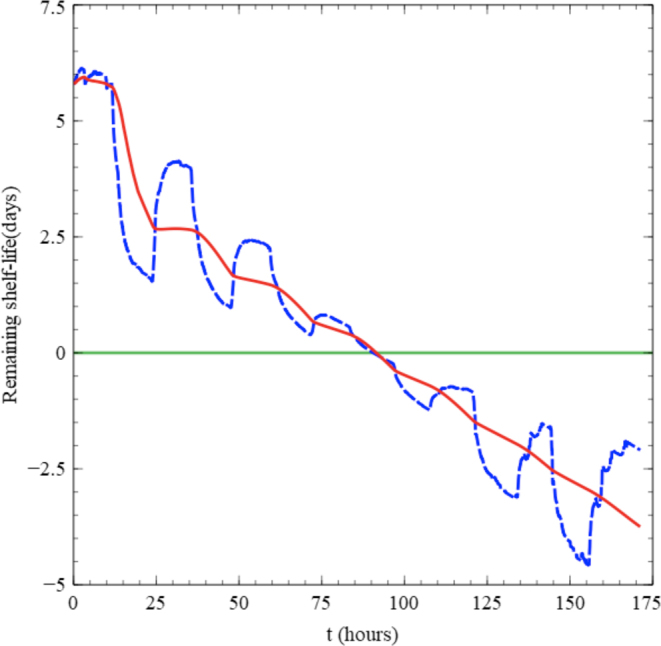
Comparison of the remaining shelf-life estimations using the mean kinetic temperature and the temperature histories under the 0 to 8°C fluctuating temperature condition during storage (), based on mean kinetic temperature ( ) based on fluctuating temperature (green line shelf-life limit).
As a remedy for this, the mean kinetic temperature was tested as the food temperature to remain for the remaining of the time of circulation. The mean kinetic temperature is the effective constant temperature to represent the impact of the fluctuating temperature history on the food quality degradation. It indicates the constant temperature at which the food quality becomes at the level of the inspecting moment tcurrent under fluctuating temperature T(t) condition as shown in Eq. (11):
| (11) |
Since N in Eq. (5) shows the food quality, it could be obtained by integrating the equation as in Eq. (12):
| (12) |
Figure 6 compares the measured temperature history and the mean kinetic temperature of the chicken meat under the considered temperature history. While the mean kinetic temperature shows large temperature change initially, it stabilizes after a couple of temperature shifts and stays at a level. Since it indicates the integrated effect of the storage, its variation decreases with the elapse of time. The solid red line in Figure 5 shows the estimation of the remaining shelf-life. Although it has a small kink initially, it shows almost monotonic decrease with time as it is expected what the remaining shelf-life would like to be.
Figure 6.

Comparison of the measured temperature and the mean kinetic temperature of the chicken meat under the 0 to 8°C fluctuating temperature condition during storage (), mean kinetic temperature (), measured temperature.
Conclusions
Total plate count was determined to have higher relationship to packaged chicken meat quality deterioration. It can be used as predictor variable for packaged chicken meat freshness and shelf-life prediction models. A mathematical model that describes the growth of TPC from 0 to 15°C was developed utilizing isothermal storage data and was validated against experimental observations under fluctuating (0–8°C) as well as real-time distribution temperature conditions and performed well. The shelf-life model developed based on MKT showed an even decrease of shelf-life under dynamic condition in time. It may be used to estimate the remaining shelf-life of packaged chicken meat under any temperature condition in the range from 0 to 15°C during its circulation.
The developed model can be implemented in real chicken meat distribution chains by adapting it to specific chicken meat distribution chain conditions. Provided that efficient temperature recording tools are available, the model can be considered to be an effective tool for quality monitoring and shelf-life management within the chicken meat supply and distribution chain.
ACKNOWLEDGMENTS
This research was supported by the Main Research Program (E0162501) of the Korea Food Research Institute (KFRI) funded by the Ministry of Science and ICT.
REFERENCES
- Baranyi J., Roberts T.A. A dynamic approach to predicting bacterial growth in food. Int. J. Food Microbial. 1994;23:277–294. doi: 10.1016/0168-1605(94)90157-0. [DOI] [PubMed] [Google Scholar]
- Baranyi J., Robinson T.P., Kaloti A., Mackey B.M. Predicting growth of Brochothrix thermosphacta at changing temperatures. Int. J. Food Microbiol. 1995;27:61–75. doi: 10.1016/0168-1605(94)00154-x. [DOI] [PubMed] [Google Scholar]
- Bruckner S., Albrecht A., Petersen B., Kreyenschmidt J. Influence of cold chain interruptions on the shelf life of fresh pork and poultry. Int. J. Food Sci. Technol. 2012;47:1639–1646. [Google Scholar]
- Bruckner S., Albrecht A., Petersen B., Kreyenschmidt J. A predictive shelf life model as a tool for the improvement of quality management in pork and poultry chains. Food Control. 2013;29:451–460. [Google Scholar]
- Choe J.H., Nam K.C., Jung S.O., Kim B.N., Yun H.J., Jo C.R. Differences in the quality characteristics between commercial Korean native chickens and broilers. Korean J. Food Sci. An. 2010;30:13–19. [Google Scholar]
- da Silva N.B., Longhia D.A., Martinsa W.F., de Aragãoa G.M.F., Carciofia B.A.M. Mathematical modeling of Lactobacillus viridescens growth in vacuum packed sliced ham under non isothermal conditions. Procedia Food Sci. 2016;7:33–36. [Google Scholar]
- Ghollasi-Mood F., Mohsenzadeh M., Hoseindokht M.R., Varidi M. Quality changes of air-packaged chicken meat stored under different temperature conditions and mathematical modelling for predicting the microbial growth and shelf life. J. Food Saf. 2016 doi: 10.1111/jfs.12331. [DOI] [Google Scholar]
- Ghollasi-Mood F., Mohsenzadeh M., Hoseindokht M.R., Varidi M. Microbial and chemical spoilage of chicken meat during storage at isothermal and fluctuation temperature under aerobic conditions. IJVST. 2017;8 doi: 10.22067/veterinary.v8i1.54563. [DOI] [Google Scholar]
- Goksoy E.O., Kirkan S., Kok F. Microbiological quality of broiler carcasses during processing in two slaughterhouses in Turkey. Poult. Sci. 2004;83:1427–1432. doi: 10.1093/ps/83.8.1427. [DOI] [PubMed] [Google Scholar]
- Gospavic R.J., Kreyenschmidt J., Bruckner S., Popov V., Haque N. Mathematical modelling for predicting the growth of Pseudomonas spp. in poultry under variable temperature conditions. Int. J. Food Microbiol. 2008;127:290–297. doi: 10.1016/j.ijfoodmicro.2008.07.022. [DOI] [PubMed] [Google Scholar]
- Grau R., Sánchez A.J., Girón J., Iborra E., Fuentes A., Barat J.M. Nondestructive assessment of freshness in packaged sliced chicken breasts using SW-NIR spectroscopy. Food Res. Int. 2011;44:331–337. [Google Scholar]
- Herbert U., Albrecht A., Kreyenschmidt J. Definition of predictor variables for MAP poultry filets stored under different temperature conditions. Poult. Sci. 2015;94:424–432. doi: 10.3382/ps/peu002. [DOI] [PubMed] [Google Scholar]
- Hong G.E., Kim J.H., Ahn S.J., Lee C.H. Changes in meat quality characteristics of the Sous-vide cooked chicken breast during refrigerated storage. Korean J. Food Sci. An. 2015;35:757–764. doi: 10.5851/kosfa.2015.35.6.757. [DOI] [PMC free article] [PubMed] [Google Scholar]
- ICMSF (Int. Commission Microbiological Specifications for Foods) In: HACCP in Microbiological Safety and Quality. Great Britain. Silliker J.H., Baired-Parker A.C., Bryan F.L., Christian J.H.B., Roberts T.A., Tompkin R.B., editors. Blackwell; London, UK: 1988. Part 1 Principles; pp. 7–12. [Google Scholar]
- ISO . 1st ed. International Organization for Standardization; Geneva, Switzerland: 1988. Sensory Analysis—General Guidance for the Design of Test Room. ISO 8589 Standard. [Google Scholar]
- ISO . 2nd ed. International Organization for Standardization; Geneva, Switzerland: 2007. Sensory analysis—General Guidance for the Design of Test Rooms. ISO 8589-2 Standard. [Google Scholar]
- KFDA . Korea Food and Drug Administration; Seoul, Korea: 2011. Korean Food Standards Codex; pp. 5.11.2–5.11.3. 10.3.1. [Google Scholar]
- Khulal U., Zhao J., Hu W., Chen Q. Intelligent evaluation of total volatile basic nitrogen (TVB-N) content in chicken meat by an improved multiple level data fusion model. Sens. Actuators B. 2017;238:337–345. [Google Scholar]
- Kreyenschmidt J. Rheinische Friedrich-Wilhelms-Universität Bonn, AgriMedia; Bergen/Dumme, Germany: 2003. Modellierung des Frischeverlustes von Fleisch sowie des Entf¨arbeprozesses von Temperatur-Zeit- Integratoren zur Festlegung von Anforderungsprofilen für die produktbegleitende Temperaturüberwachung. PhD Thesis. [Google Scholar]
- Park H.R., Kim Y.A., Jung S.W., Kim H.C., Lee S.J. Response of microbial time temperature indicator to quality indices of chicken breast meat during storage. Food Sci. Biotechnol. 2013;22:1145–1152. [Google Scholar]
- R Development Core Team . R Foundation for Statistical Computing; Vienna, Austria: 2011. R A Language and Environment for Statistical Computing.Available at: http//www.R-project.org [Google Scholar]
- Ross T. Indices for performance evaluation of predictive models in food microbiology. J. Appl. Bacteriol. 1996;81:501–508. doi: 10.1111/j.1365-2672.1996.tb03539.x. [DOI] [PubMed] [Google Scholar]
- SAS . SAS Institute Inc.; Cary, NC: 2008. SAS/STAT User's Guide. Version 9.2. [Google Scholar]
- Smolander M., Alakomi H.L., Ritvanen J., Ahvenainen R. Monitoring of the quality of modified atmosphere packaged broiler chicken cuts stored in different temperature conditions. A. Time–temperature indicators as quality-indicating tools. Food Control. 2004;15:217–229. [Google Scholar]
- Swinnen I.A.M., Bernaerts K., Dens E.J.J., Geeraerd A.H., Van Impe J.F. Predictive modeling of the microbial lag phase a review. Int. J. Food Microbiol. 2004;94:137–159. doi: 10.1016/j.ijfoodmicro.2004.01.006. [DOI] [PubMed] [Google Scholar]
- Tuncer B., Sireli U.T. Microbial growth on broiler carcasses stored at different temperatures after air- or water-chilling. Poult. Sci. 2008;87:793–799. doi: 10.3382/ps.2007-00057. [DOI] [PubMed] [Google Scholar]
- Vaikousi H., Biliaderis C.G., Koutsoumanis K.P. Applicability of a microbial time-temperature indicator (TTI) for monitoring spoilage of modified atmosphere packed minced meat. Int. J. Food Microbiol. 2009;133:272–278. doi: 10.1016/j.ijfoodmicro.2009.05.030. [DOI] [PubMed] [Google Scholar]
- Van Impe J.F., Poschet F., Geeraerd A.H., Vereecken K.M. Towards a novel class of predictive microbial growth models. Int. J. Food Microbiol. 2005;100:97–105. doi: 10.1016/j.ijfoodmicro.2004.10.007. [DOI] [PubMed] [Google Scholar]
- Witte V.C., Krause G.F., Bailey M.E. A new extraction method for determining 2-thiobarbituric acid values of port and beef during storage. J. Food Sci. 1970;35:582–585. [Google Scholar]
- Yang S., Park S.Y., Ha S.D. A predictive growth model of Aeromonas hydrophila on chicken breasts under various storage temperatures. Food Sci. Technol. 2016;69:98–103. [Google Scholar]
- Zhang Q.Q., Han Y., Cao J.X., Zhou G.H., Zhang W.Y. The spoilage of air-packaged broiler meat during storage at normal and fluctuating storage temperatures. Poult. Sci. 2012;91:208–214. doi: 10.3382/ps.2011-01519. [DOI] [PubMed] [Google Scholar]
- Zhao J., Gao J., Chen F., Ren F., Dai R., Liu Y., Li X. Modeling and predicting the effect of temperature on the growth of Proteus mirabilis in chicken. J. Microbiol. Meth. 2014;99:38–43. doi: 10.1016/j.mimet.2014.01.016. [DOI] [PubMed] [Google Scholar]