Abstract
The inefficiencies and uncertainties surrounding solutions from existing inversion methods have necessitated investigation for more efficient techniques for the inversion of ill-posed magnetic problems. In this study, the Social Spider Optimization (SSO) algorithm has been modified, adopted and successfully used in modelling physical characteristics of magnetic anomalies originating from simple-shaped geologic structures. The study, aimed at testing the capacity and efficiency of the SSO algorithm to model magnetic data of varying complexity, was successfully conducted on both synthetic data with varying levels of noise and real field data obtained from mining fields in Senegal and Egypt. To assess the mathematical nature of the inverse problem considered, error energy maps were produced for each model parameter pairs in the synthetic examples. These maps enabled the pre-assessment of the resolvability model parameter for the ill-posed problem. In addition, uncertainty analysis aimed at providing insight to the reliability of the obtained solutions was carried out using the Metropolis–Hastings (M–H) sampling algorithm. Results show that the procedure converges fast and generates accurate results even when confronted with constrained multi-parameter non-linear inversion problems. Its outstanding converging speed and accuracy of the results reveal it as an excellent procedure for overcoming agelong problems of local optimal solutions associated with pre-existing algorithms. The consistency of the results with actual values affirms the efficacy of the new procedure which is pioneering in geophysical literature. It is therefore a stable and efficient tool for performing geophysical data inversion and is therefore recommended for use in inverting geophysical data with higher complexities like seismic reflection and gravity data, that require many corrections to be performed before reliable geological interpretations can be made.
Keywords: SSO, Optimization, Modelling, Magnetics, Geologic structure, Noise
SSO; Optimization; Modelling; Magnetics; Geologic structure; Noise.
1. Introduction
Traditionally, geological modelling focuses mainly on assembling geological information (ichnography, thin sections, regional geology maps and lithology logs from drill cuttings) in generating subsurface models. Models generated from this approach are usually very accurate and reliable but the process of acquiring these data, particularly in unexplored fields, is usually laborious, time consuming and expensive. Hence, the indirect geophysical approach was introduced. Geophysical data are usually acquired for use in modelling and imaging geologic structures buried at various depths below the Earth's surface. Data useful for geophysical modelling of geological structures are usually acquired in a systematic manner under controlled conditions and the outcome, which can be presented either in profile or numerical values, represents observations at fixed or random positions. The geophysical exploration methods are many and each method exploits variations in physical properties of rocks in mapping the dimensions of an anomalous geologic structure buried at various depths. The properties of such anomalous structure differ from those of its surrounding environment with respect to composition, texture and/or source.
Amongst all the conventional geophysical techniques, magnetic method is the oldest, simplest and most reliable method commonly used in the search for both hidden ores and structures associated with mineral deposits (Sharma, 1987). Recently, with the fast rate in which most known surficial mineral deposits are being depleted, the magnetic method has gained enormous applications in delineating structural boundaries beneath sediments economically and in exploring for new mineral reserves (Ekwok et al., 2020; Shayanfar et al., 2016). Information obtained from the mapping of such structural boundaries serve as controls in the analysis of frontier sedimentary basin areas (Ekwok et al., 2019; Rezouki et al., 2020; Ganguli et al., 2020).
The measurable parameters, which include spatial variations in magnetic field strengths usually generated from field surveys and dips, are always processed to free the raw field data of the few contributions from extraneous sources in the best possible ways. The techniques of processing magnetic data, filtering, display and interpretation have been advanced with the advent and application of high-speed computers, artificial intelligence and colour raster graphics. The processed data are analyzed and interpreted in terms of the depths of burial, geometry and magnetic properties of the causative bodies. Interpreters have high confidence level in the geological and structural interpretation of inverted magnetic data.
Inversion of magnetic data is a stepwise modeling process that seeks to determine characteristic physical parameters of a buried geologic structure by assuming their similarities to known and/or pre-defined models (Kaftan, 2017). The structures of interest in geological exploration usually include spheres, infinitely long cylinders, thin sheets and geological contacts, and all modelling procedures seek to determine the parameters that define their latent physical characteristics of depth, position and shape (amplitude and dip angle) of the observed structure. Over the years, reports of the application of different techniques in determining these parameters have been made. These procedures are united by adept functional exploitation of computational approaches including Euler deconvolution (Essa et al., 2020; Mota et al., 2020; Nuamah Daniel and Tandoh Kingsley, 2020), Werner deconvolution (Ekwok et al., 2019, 2020; Essa et al., 2020), model layering (Pilkington, 2006) and parametric curves (Abdelrahman et al., 2012). Others make use of fair function minimization procedure and Depth from Extreme Points (DEXP) (Fedi, 2007; Tlas and Asfahani, 2011), linear least squares approach (Abo-Ezz and Essa, 2016) and simplex algorithm (Tlas and Asfahani, 2015). However, practitioners have shown that results obtained from these conventional gradient-based inversion approaches usually lead to the generation of large numbers of invalid solutions caused by many factors including noise sensitiveness and poor window size compatibility (Essa and Elhussein, 2018, 2020). Other causes include improper filtering of noise from signals of interest (Zhdanov, 2002; Mbonu et al., 2021) and over dependence on initial model parameters from subjective prior geologic information (Cai and Zhdanov, 2015) which may not be reliable or sufficiently reputable.
Several attempts have been made to resolve these challenges without much success as given by Mosegaard and Tarantola (2002), Scales and Tenorio (2001) and Snieder (2019) but with rapid improvements in machine learning and artificial intelligence (Ewees et al., 2017), practitioners have shown that, using the instrumentality of the more recent and stable evolutionary techniques, these perennial inversion problems are gradually being overcome. Kaftan (2017) employed genetic algorithm (GA) for the optimal interpretation of magnetic anomalies caused by surficial sources, Essa and Elhussein (2018) employed particle swarm optimization (PSO) technique in interpretating magnetic anomalies caused by sources with simple geometrically-shaped structures Balkaya et al. (2017) conducted three dimensional non-linear inversion of magnetic anomalies originating from prismatic bodies using differential evolution algorithm, Srivastava and Agarwal (2010) employed the ant colony optimization (ACO) technique in inverting the amplitude of a two-dimensional analytic signal from magnetic anomaly. Gö kt ü rkler and Balkaya (2012) employed a combination of three global optimization techniques (GA, PSO and simulated annealing, SA) to comparatively assess the accuracy of estimates made from the metaheuristics-based stochastic methodologies over their gradient-based counterparts. Di Maio et al. (2016) employed a robust genetic-price algorithm in inverting self-potential data while Gobashy et al. (2020) utilised the whale optimization algorithm (Mirjalili et al., 2016) in interpreting magnetic anomalies due to dike-like and vertical fault like/shear structures with different orientations and geologic features. Other studies involving metaheuristic procedure include Ben et al. (2021a), Ben et al. (2022) and Ben et al. (2021c), who adopted the recently introduced manta ray foraging optimization for the estimation of model parameters due to shallow and deep-seated structures from potential field data. In addition, Ekinci and Yiʇitbaş (2015) and Ekinci et al. (2017) studied the prospects of applying and the effectiveness of the differential evolution (DE) algorithm in evaluating magnetic anomalies due to both hypothetical and real-isolated geological bodies. While Ekinci et al. (2015) focused on residual gravity anomalies, Ekinci et al. (2017) experimented with analytic signal of magnetic anomalies. Consequent upon the satisfactory performance of the DE procedure with isolated anomaly cases, Ekinci et al. (2020) adapted the algorithm for extensive basement relief delineation of the Aegean Graben system. These bioinspired intelligent algorithms, which claim to work by the functional imitation of the normal behaviour of animals or groups of animals, are more efficient in overcoming these challenges. The strength of these algorithms is drawn from the fact that they are conditioned to be zero-order implying that any performance enhancements made in a direction towards feasible solution is not related to the derivatives of the function minimized or in some cases, maximized.
The Social Spider Optimization (SSO) is a population based algorithm that mimics the cooperative behavioural style of social spiders (Arul Xavier and Annadurai, 2019; Pradhan et al., 2018). SSO algorithm exploits the behaviour of both male and female spiders concurrently searching for space in their operations. The location of each individual spider (agent) is adjusted with sets of bio-guided evolutionary operators, which depend on the gender of the agent, in searching for an optimal solution that satisfies the objective. As the algorithm mimics individually categorized traits as against swarm traits, the collective cooperative colony behavioural results of this personalized characterization is healthy reductions in critical particle concentration defects that are commonly observed in several evolutionary algorithm procedures (such as PSO, GA and ACO (Majumder et al., 2018; Ewees et al., 2017; Klein et al., 2016; Sanyi et al., 2009)). Examples of such defects include exploration-exploitation imbalances and suboptimal solutions from premature convergences. This computational edge has motivated the successful application of SSO in diverse fields of engineering (Husodo et al., 2020; Arul Xavier and Annadurai, 2019; Shayanfar et al., 2016), image processing (Cuevas et al., 2018; Bhandari et al., 2018; Akram & Abd-AlKareem, 2018; Ouadfel and Taleb-Ahmed, 2016) and energy (Alrashidi et al., 2020; Ewees et al., 2017) amongst others. Records of applications of SSO procedure in these fields of research, increasingly promise the algorithm promises to be a meaningful and appropriate inversion tool for geophysical data inversion. However, to the best of the authors’ shared knowledge, there has been no reports of its application in geophysical data inversion. Thus, the novelty of this study lies in the pioneering application of the SSO in modelling geophysical data.
Therefore, in this paper, we pioneered the application of the SSO algorithm in the inversion of magnetic data in order to assess the distribution of magnetic properties over simple geometrical causative sources. The paper begins with the methodology of magnetic inversion and social spider optimization technique. The technique is then demonstrated by applying it to synthetic models corrupted with different levels of Gaussian noise (0, 10, 20 and 20%) and multi/integrated anomaly models. Next, the new methodology is applied to two real life Case studies from mining sites in Senegal and Egypt. The parameter values obtained are then compared with those obtained from similar studies conducted using conventional techniques as well as from drilling information. Furthermore, and to clarify uncertainties in the solutions, model parameters from the magnetic anomalies were compared with the results obtained with the Metropolis–Hastings (M–H) sampling algorithm using the simulated annealing without a cooling scheme. Finally, the paper is concluded with a brief analysis of the performance and applicability of SSO as a magnetic anomaly inversion tool.
2. Methodology
2.1. Magnetic inversion and two-dimensional anomaly problem
In the field of Geophysics, inversion is commonly achieved through the transformation of ill-posed problems into optimization scenarios where model parameters, describing the buried geologic structures, as long as a good fit with the observed data is attained (Tarantola, 2005). The inverse solution requires the supposition of an initial model (Mehanee, 2014; Zhdanov, 2002). A promising initial model could be made by introducing a priori information from geology, drilling or other geophysical techniques (Mehanee and Essa, 2015).
Information on the initial model is commonly obtained from geologic, drilling or previous geophysical data (Sun et al., 2019). The data are usually subjected to gradual smoothening in a stepwise running iteration until a subjectively acceptable fit between the estimated and measured data is obtained. Then, smoothening is done by intelligent forward-adjustment of the model parameters. For magnetic inversion, the required model parameters are typically the amplitude coefficients (K), which is related to the thickness of the body, the depth (d) to the geologic structure from the surface, coordinate location of the another at the origin (xo), the shape factor related to the shape of the body and the angle of magnetization.
2.2. The generalized expression
The generalized expression for a two dimensional magnetic anomaly along a profile, T (xk, K, d, α, xo, p), for simple geometric shapes (equation 1) was used in this study. Eq. (1) was obtained by Abdelrahman and Essa (2015) after adding contributions to the total magnetic anomalies from spherical objects (Rao et al., 1977; Prakasa Rao and Subrahmanyam, 1988), thin sheets (Gay, 1963) and horizontal cylinders (Rao et al., 1986).
| (1) |
where, d denotes depth to the buried body from the surface, N is the number of data points and K is the amplitude coefficient of the body. xo represents the coordinate location of the center of the causative anomaly. A, B and C are defined as shown in Eq. (2) (Essa and Elhussein, 2018)
| (2) |
where, α is the angle of effective magnetization. Rao et al. (1973) and Prakasa Rao and Subrahmanyam (1988) determined the range of α values for spherical anomalies, while Gay (1963) calculated α values for thin sheet and horizontal cylinder anomalies. FSD and SHD are first and second horizontal derivatives, respectively, while p is the shape factor with values of 1.0, 2.0 and 2.5 for thin sheet, horizontal cylinder and sphere, respectively (Abdelrahman and Essa, 2015). These five parameters- K, d, α, xo, and p, are the model parameters that will be determined in this study using the SSO procedure. Optimal values of the model parameters that minimize the differences between the estimated and observed data were computed using a simple objective function in nT, Eq. (3) (Essa and Elhussein, 2020) as
| (3) |
where, Tkm and Tkc (estimated using the SSO procedure) are measured and estimated magnetic anomalies.
2.3. Social spider optimization
Social Spider Optimization is a heuristic optimization algorithm introduced by Cuevas et al. (2013). The algorithm operates by mimicking the cooperative behavior of social spiders where both the male and female spiders work together as search agents. The spiders moves randomly within the search space in a high-dimensional communal spider web where each spider is touted as a candidate solution (Alrashidi et al., 2020). The algorithm, designed to use their behavioral pattern in solving the magnetic inversion problem, was implemented in seven steps as follows:
Step 1
First, the male and female population vectors of spiders (representing magnetic models or search agents) were randomly initiated in search space. Each member of this population is taken as a prospective solution to our geophysical problem. Considering the fact that the density of female spiders are usually more than the density of male spiders (about 65–90% of the whole population of the colony), the number of female spiders, Nf was generated using Eq. (4) (Yu and Li, 2015) as
(4) where, rand is a random number in the range [0,1] and Floor is a function that returns the largest integer that is less than or equal to N (the total number of spiders in the search space). The number of males spiders then becomes Nm = N - Nf. We also assumed that the population denoted as S contains N elements where, S = F ∪ M such that S = {s1, s2,…, sN}), and S = {s1 = f1, s2 = f2, …, sNf = fNf.sNf+1 = m2,…, sN = mNm}.
Step 2
Weight, Z1 was assigned to all the spiders. This weight defines the quality of spiders in the population S. Z1 was determined from Eq. (5) as
(5) where, Q is the fitness value of a spider evaluated using the objective function while worsts and bests corresponds to the worst and best individual spiders in the population, respectively. The bests and worsts were defined by Eqs. (6) and (7) as
(6)
(7)
Step 3
The movement of spiders synonymous with their vibration (VIB process) is simulated. This procedure was implemented using Eq. (8) (Husodo et al., 2020; Mirjalili et al., 2016) as
(8) where, Di,j is the Euclidian distance between spiders i and j.
Step 4
The position of the models, as denoted by the spiders, was initialized. The position vector for each spider, fi or mi, is a 5-dimensional vector populated by the parameters to be optimized (K, d, α, xo, p). The values of these parameters were randomly generated within the some predefined upper, and lower, bounds (Eqs. (9) and (10))
(9)
(10) where, n is the number of parameters; (n = 5 in this study).
Step 5
For each iterative session, the co-operative interaction between individual spiders in the colony was implemented according to the spider gender using Eq. (11).
(11) where, Xi and Ck are the dataset and clustering center vectors, respectively. Since the direction of movement of spiders (towards or away) from each other depends mainly on neighboring spider's vibration, the movement was modeled using Eq. (12) (Akram & Abd-AlKareem, 2018; Ben et al., 2021b; Bhandari et al., 2018) as
(12) where, α, β, δ and r are random numbers within the range of 0 and 1, k is the total number of maximum iterations, TV is the threshold value otherwise known as the probability factor, and sc and sb are the nearest best spider to spider i, and the best spider in the entire population S, respectively.
Step 6
The co-operative behavior of male spiders was defined. In natural spider colonies, males are categorized into dominant and non-dominant males. The dominant males characterized by high fitness values usually stand better chances of attracting female partners, while the non-dominant ones, rather tend to gather in male population centers to exploit leftovers or resources lost by the dominant ones. These behaviours were simulated using Eq. (13) (Husodo et al., 2020; Mirjalili et al., 2016; Pradhan et al., 2018) as
(13) where, Sf is the nearest female spider to male spider i and the term represents the mean value of the male spiders M in the population.
Step 7
We proceeded to select best spiders to represent the offspring generation, as part of the model's evolution to solution. Within a certain radius, computed from Eq. (14) (Klein et al., 2016), mating between dominant male and female spiders was allowed in order to produce next generation of stronger spiders. The fitness values of the new generation of dominant spiders produced from the mating process were assessed and compared with those of their parents. If new spiders have better quality than their parents, then the new spiders were adopted and their parents were discarded.
(14) where, n represents the problem dimension, and and are the upper and lower bounds, respectively. In this study, the ranges of the upper and lower bounds for each of the parameters were selected based on subjective deductions from prior geological or geophysical information. Examples of these deductions are those giving insights as to what geologic materials are commonly found in the region, the range of depth that they are usually found and the regional/local tectonic history of the region - that may give insights as to the angle of dip of the buried structure).
At the end of every successive iteration, the quality of results obtained in that particular stage was evaluated by calculating the misfit between the estimated and measured parameters from Eq. (15), which is basically the root mean square error of the inversion process.
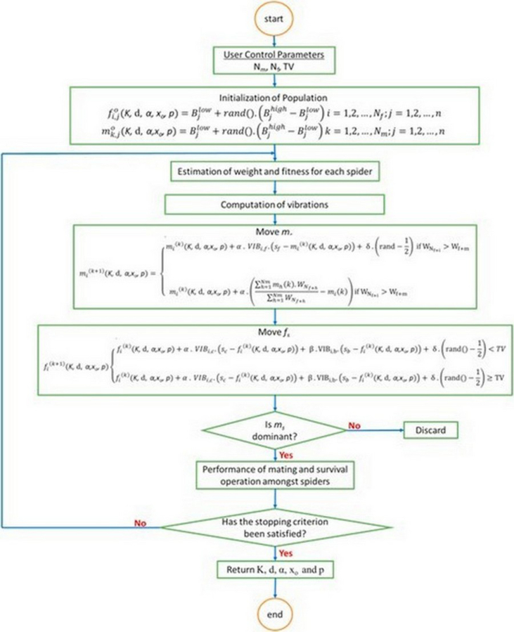
(15) Figure 1 shows a simplified flowchart showing the steps used in implementing the SSO optimization process.
Figure 1.
A simplified flowchart showing main steps used in implementing the SSO algorithm.
2.4. Uncertainty analysis
Since the geophysical inverse problems are mostly illposed, non-unique, and nonlinear, a wide range of Earth models from obtainable different sets of parameters can concurrently adapt to measurement data. A Bayesian methodology, which focuses on estimating conditional probabilities, can be used to approximate model parameters reflecting random changes. By combining the probability of observed data with background understanding, the method allows previous distribution of the so-called parameters to be achieved. Correct sampling has been achieved using the Markov chain-monte carlo algorithm with global optimization algorithms such as GA, SA, and PSO (Alvarez et al., 2008; Fernández Martinez et al., 2010; Mosegaard and Tarantola, 1995; Sen and Stoffa, 2013). For analysis in this study, the Metropolis-Hasting sampling algorithm (M-H) was adopted for model parameter sampling. The M-H algorithm which was originally introduced by Metropolis et al. (1953); then generalized by Hastings (1970) principally suggests different but related models using previous related outputs of the distribution. In all cases, the probability was determined for each new model by resolving the forward problem and calculating the misfit in the data. If the likelihood increases, the new model was deemed suitable. Furthermore, even though the likelihood decreased, the current model was still adopted, howbeit with a probability based on the likelihood ratio between the original model and the one suggested.
The algorithm, which is based on simulated annealing without cooling (Alvarez et al., 2008), allows for uncertainty assessment by presenting confidence intervals based on parameters.
2.5. Algorithm configuration/processing time
The code used in implementing the SSO algorithm was configured in PYTHON using the virtual studio algorithm compiler. It was installed on a simple desktop PC running on windows 10 with Core i5 processor. The duration of compilation depends on the complexity of the model structure. For simple models, the iteration process terminated within 1–2 min. However, there was an increase in processing time (up to 20%) for multi-model cases.
3. Synthetic examples
The SSO algorithm's dependability and reliability were investigated by subjecting it to a series of credibility tests using both simulated noise-free models (thin-sheet, horizontal cylinder, and sphere) and later, intentionally induced noisy models.
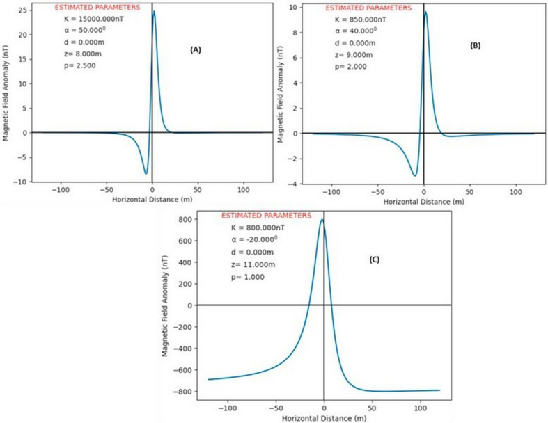
Most nature-inspired global optimization algorithms have their own control parameters that heavily influence the algorithm's convergence point during inversion. These parameters are critical for any algorithm's overall efficiency (Pekşen et al., 2014; Ekinci et al., 2016, 2017). Their selection, however, is largely determined by the essence of the considered problem (Balkaya et al., 2017). As a result, prior to inversion, model parameters tunings were carried out to choose the best control parameters for the algorithm. A synthetic magnetic anomaly dataset was theoretically developed for a spherical model (Figure 2A) using Eq. (1) with K = 15000 nT, d = 8 m, p = 2.5, = 50o, xo = 0 m, and profile length of 100 m for proper guidance during the tuning studies. The parameter tuning analyses were primarily concerned with determining the best values for the likelihood factor – TV – and the spider population – N in the search space. For the model parameters, large search spaces (Table 1) were used. This was to help in the investigation of the impact of TV on the final solution. Thirty independent runs were carried out with N = 150 and 1000 iterations for optimization. N was calculated by multiplying the number of independent runs (30) by the number of unknown model parameters (5). The magnetic anomaly problem was then statistically evaluated using the minimum, mean, and standard deviation of RMS values obtained from several independent runs. Table 2 displays the results obtained by using different TV values after 30 runs. The table shows that using a TV value of 0.7 yielded the most optimal statistical outcomes (bold face). This means that if 0.7 is used as the probability factor for the magnetic data, the optimization process will be more stable and efficient. Consequently, 0.7 was adopted as the best PV for the optimization problem.
Figure 2.
Theoretically generated noise-free anomaly for (A) Sphere Model (B) Horizontal Cylinder Model (C) Thin Sheet Model.
Table 1.
Estimated parameters for the noise-free synthetically generated models.
| Type of model | Parameters | Parameter bounds | TRUE | Estimated |
|---|---|---|---|---|
| Sphere | K (nT) | 5000–30000 | 15000.0 | 15000.00 |
| α (o) | −90–90 | 50.0 | 50.00 | |
| d (m) | 3–15 | 8.0 | 8.00 | |
| xo (m) | −30–30 | 0.0 | 0.00 | |
| p | 0–5 | 2.5 | 2.50 | |
| Horizontal cylinder | K (nT) | 1000–9000 | 850.0 | 850.00 |
| α (o) | −90–90 | 40.0 | 40.99 | |
| d (m) | 3–15 | 9.0 | 9.00 | |
| xo (m) | −30–30 | 0.0 | 0.02 | |
| p | 0–5 | 2.0 | 2.00 | |
| Thin sheet | K (nT) | 100–2000 | 800.0 | 800.00 |
| α (o) | −90–90 | −20.0 | −20.00 | |
| d (m) | 0–30 | 11.0 | 11.00 | |
| xo (m) | −30–30 | 0.0 | 0.00 | |
| p | 0–5 | 1.0 | 0.99 |
Table 2.
Results of parameter tuning studies.
| TV | RMS (nT) |
||
|---|---|---|---|
| minimum | mean | standard deviation | |
| 0.4 | 1.42101 | 1.50843 | 0.82688 |
| 0.5 | 0.25584 | 0.43459 | 0.15284 |
| 0.6 | 0.15816 | 0.21358 | 0.0758 |
| 0.7 | 0.06953 | 0.06942 | 3.30718 × 10⁻⁷ |
| 0.8 | 0.09384 | 0.09875 | 1.61454 × 10⁻² |
| 0.9 | 0.2691 | 0.43913 | 0.1648 |
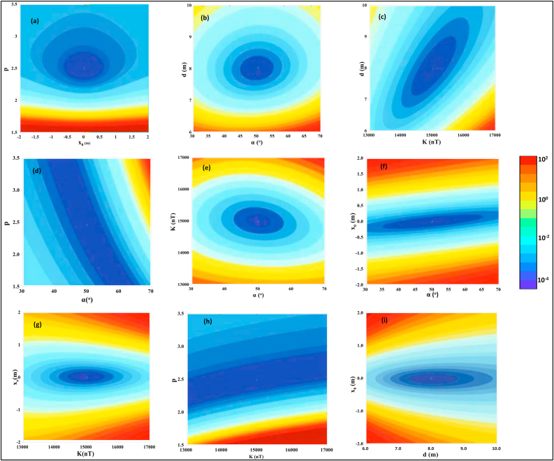
Furthermore, prediction error maps were created to aid in deciphering the resolvability and improving understanding of the relationship between the different model parameter pairs. To carry out this procedure, unused parameter values were set to their real values, and with the true parameter as the mean, parameter spaces with relatively small ranges between the minimum and maximum values were used to observe how the error surfaces circumvent the global minima. The limits of the horizontal and vertical axis were set to be equal to the search space boundaries of each parameter. White crosses show the true solutions (Figure 3). These maps show the possible positions of the model parameter solutions inside the lowest error area surrounded by the minimum contour value. It is worth noting that the shapes of these lowest error areas are major indications providing insight into the resolvability of each parameter. Figure 3 (a,b,e,g, and h) depicts near-circular contour lines encircling the lowest error surfaces for some parameter pairs. This behaviour explicitly shows that the associated model parameter is unrelated to the others and can thus be resolved independently. The elliptical surface contours that sloping towards one of the parameter axes (Figure 3 c, f and i) indicate positive or negative correlations and interpretatively reveal dependency relationship between the parameters. This relationship means that reliable estimation of one parameter is dependent on accurate estimation of others. In cases where there is a positive association between any two pairs of model parameters, a change in the value of one parameter can cause a proportional change in the value of the other parameter for appropriate estimations. The parameter solutions' dependencies are shown by the sloping (unclosed) contours (Figure 3d and h). According to Ekinci et al. (2020), unclosed contour behaviors are typically distinguished by complicated optimization due to the presence of identical solutions with the same error values in the narrow valley topography. In the Case of the present parameter estimation study, no major difficulties were found because the topography of constructed error energy maps did not include cases of parallel contours. Because of the similarity in the construction of numerical representations of cylinders and thin sheets with the sphere model, error plots for these three cases were observed to show very similar features; thus, the plots for the first two are not replicated here for brevity.
Figure 3.
Error energy maps for sphere model parameter pairs (a) xo-p, (b) α-d, (c) K-d, (d) α-p, (e) α-K, (f) α-xo, (g) K-xo, (h) K-p, (i) d-xo.
3.1. Noise-free models
The SSO method was used to model noise-free (synthetic) magnetic anomalies caused by basic geometrical shapes. The models are as follows: a spherical model with K = 15000 nT, d = 8 m, p = 2.5, = 50o, xo = 0 m and a profile length of 100 m; a horizontal cylinder with K = 4000 nT, d = 7 m, = 40o, p = 2, xo = 0 m and a profile length of 240 m; and a thin sheet with K = , xo = 0 m and profile length of 90 m Eq. (1) was used to calculate the magnetic field anomalies caused by these geometrical shaped anomalies (Figure 2).
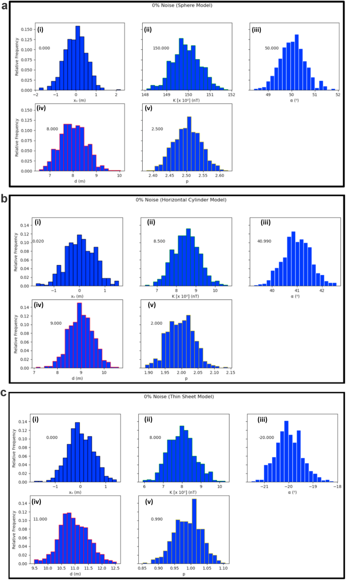
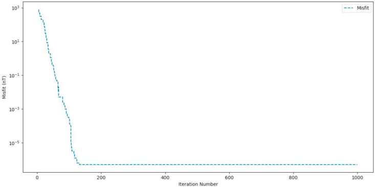
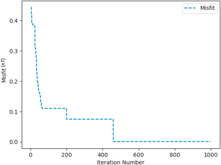
The search space was seeded with 150 initial models/vector spiders and a diverse set of parameter boundaries. K values for spherical deviations were set to be between 5,000 and 30,000 nT, d between 3 and 15 m, α between -90o to 90o, p between 0.5 and 3.5, and xo between - 30 and 30 m. K values for the horizontal cylinder model range from 1,000 to 9,000 nT, d from 3 to 15 m, -90o to 90o, p from 0 to 5, and xo from -30 to 30 m. Lastly, in the thin sheet model, K values were varied between 100 and 2000 nT, d between 0 and 30 m, -90o to 90o, p between 0 and 5, and xo between -30 and 30 m. Each algorithm was allowed to run a total of 1000 repeated iterations (Figures 4,5,6,7, 8). The observed values for the five model parameters (K, d, p, xo) were found to be in close alignment with their known values (Tables 1 and 3). Furthermore, a careful examination of the histogram reconstructed using the M-H algorithm's uncertainty appraisal technique (Figures 4a, 5a, 6a, 7a) reveals that our solutions fall within very reasonable confidence intervals.
Figure 4.
a: Histogram reconstructions by Metropolis –Hasting algorithm based on noiseless model datasets (Sphere Model) – (i) Origin (ii) Amplitude coefficient (iii) Angle of effective magnetization (iv) depth (v) Shape factor. b: Histogram reconstructions by Metropolis –Hasting algorithm based on noiseless model datasets (Horizontal Cylinder Model) – (i) Origin (ii) Amplitude coefficient (iii) Angle of effective magnetization (iv) depth (v) Shape factor. c: Histogram reconstructions by Metropolis –Hasting algorithm based on noiseless model datasets (Thin Sheet Model) – (i) Origin (ii) Amplitude coefficient (iii) Angle of effective magnetization (iv) depth (v) Shape factor.
Figure 5.
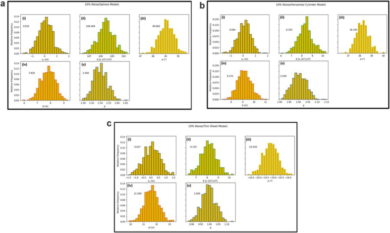
a: Histogram reconstructions by Metropolis –Hasting algorithm based on model datasets (Sphere Model) with 10% noise – (i) Origin (ii) Amplitude coefficient (iii) Angle of effective magnetization (iv) depth (v) Shape factor. b: Histogram reconstructions by Metropolis –Hasting algorithm based on model datasets (Horizontal Cylinder Model) with 10% noise – (i) Origin (ii) Amplitude coefficient (iii) Angle of effective magnetization (iv) depth (v) Shape factor. c: Histogram reconstructions by Metropolis –Hasting algorithm based on model datasets (Thin Sheet Model) with 10% noise – (i) Origin (ii) Amplitude coefficient (iii) Angle of effective magnetization (iv) depth (v) Shape factor.
Figure 6.
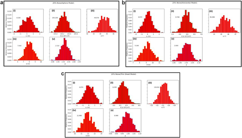
a: Histogram reconstructions by Metropolis –Hasting algorithm based on model datasets (Sphere Model) with 20% noise – (i) Origin (ii) Amplitude coefficient (iii) Angle of effective magnetization (iv) depth (v) Shape factor. b: Histogram reconstructions by Metropolis –Hasting algorithm based on model datasets (Horizontal Cylinder Model) with 20% noise – (i) Origin (ii) Amplitude coefficient (iii) Angle of effective magnetization (iv) depth (v) Shape factor. c: Histogram reconstructions by Metropolis –Hasting algorithm based on model datasets (Thin Sheet Model) with 20% noise – (i) Origin (ii) Amplitude coefficient (iii) Angle of effective magnetization (iv) depth (v) Shape factor.
Figure 7.
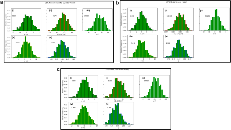
a: Histogram reconstructions by Metropolis –Hasting algorithm based on model datasets (Horizontal Sheet Model) with 25% noise – (i) Origin (ii) Amplitude coefficient (iii) Angle of effective magnetization (iv) depth (v) Shape factor. b: Histogram reconstructions by Metropolis –Hasting algorithm based on model datasets (Sphere Model) with 25% noise – (i) Origin (ii) Amplitude coefficient (iii) Angle of effective magnetization (iv) depth (v) Shape factor. c: Histogram reconstructions by Metropolis –Hasting algorithm based on model datasets (Thin Sheet Model) with 25% noise – (i) Origin (ii) Amplitude coefficient (iii) Angle of effective magnetization (iv) depth (v) Shape factor.
Figure 8.
Convergence curve for Synthetic Anomaly (Sphere, 0% noise).
Table 3.
The best statistical results obtained from the SSO algorithm for the synthetically-generated models after 30 independent runs.
| STATISTICS | Sphere Model | Horizontal Cylinder | Thin Sheet | |
|---|---|---|---|---|
| RMS (nT) | Minimum Mean Standard Deviation |
0.06953 0.06942 3. 30718 × 10−7 |
0.09746 0.11647 2..4641 × 10−5 |
0.04937 0.06543 4.9842 × 10⁻⁸ |
| Total Elapsed Time (seconds) | 62 | 67 | 59 |
3.2. Noisy models
To simulate subsurface conditions in non-ideal geologic scenarios, the synthetic anomalies of the three forward models were deliberately contaminated with normally distributed and zero-meaned pseudo-random numbers with standard deviation of ±2 nT. Each noise level (10, 20 and 25%) was obtained independently by scaling the synthetic noise-free magnetic anomaly. The authors employed the SCILAB PYTHON library to achieve this. The purpose of embedding these varying levels of noise in the noise-free anomaly was to monitor/assess the performance of SSO algorithm in the presence of noise due to the host rock or intercalating geologic materials. The noise percentage was computed using Eq. (16).
| (16) |
where, T and Tn are vectors of the noise-free and noisy anomalies, respectively.
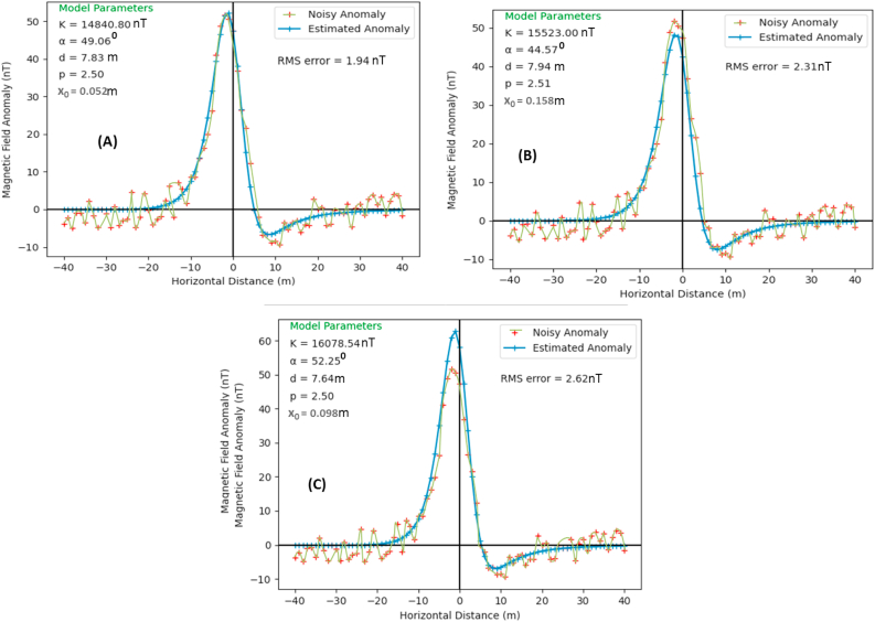
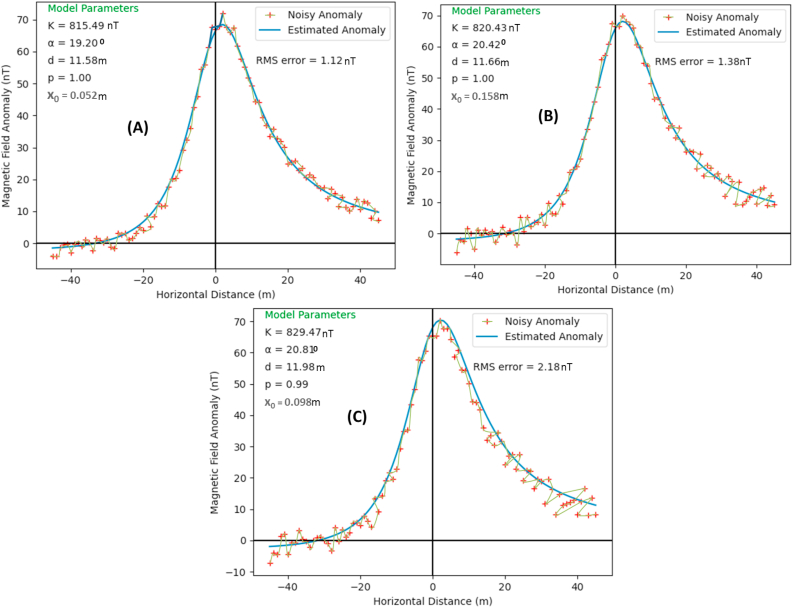
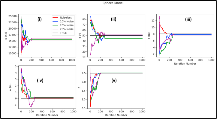
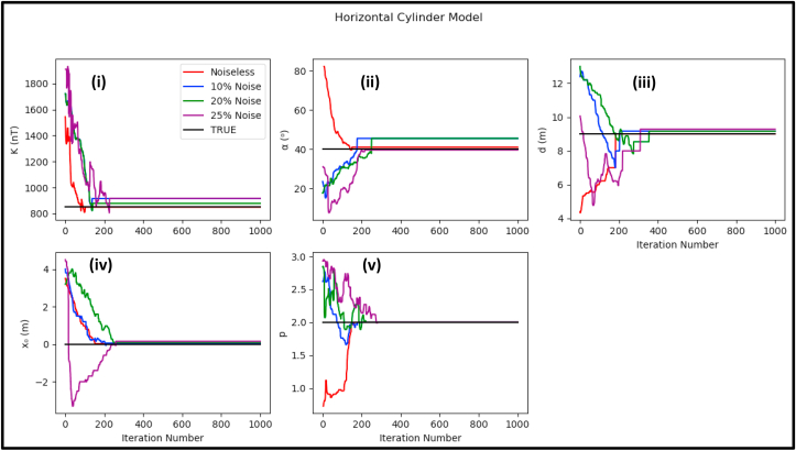
The SSO algorithm was again used in estimating the model parameters using the objective function (equation 2). In all cases, the upper and lower bounds of the model parameters were consistent with those listed in Section 3.1. After every successive iteration, the convergence and level of misfit were carefully analyzed. At the end of the execution of the SSO algorithm, the difference between the estimated and actual model parameters were observed to be insignificant (Figures 9 and 10). After converging (Figures 11, 12, 13, and 14), the level of misfit at the end of each successive run, as measured using the RMS error technique, increases marginally with increase in noise level. However, this slight increase did not affect the integrity of the inversion process as the estimated results of the model parameters (K, d, α, p, xo) remain consistent even up to the high noise level of 25% (Table 3). More too, the RMS error values (Figures 9, 10, 15) are found to be well-matched to the STD at all levels of artificially added noise content. These observations uniquely capture the capacity of the SSO algorithm to suppress noise, thereby affirming its stability and efficiency for optimal inversion of magnetic anomalies. Their higher convergence speed and accuracy mark them out as better tools for overcoming problems of local optimal solutions associated with other procedures like the quasi-Newton method and Levenberg- Marquardt method (Sanyi et al., 2009). The observed histogram construction of model parameters for all cases of the executed noisy models is displayed in Figures 11, 12, and 13. Careful consideration of each of the observed histograms by the Metropolis-Hasting sampler (Figures Figure 4, Figure 5, Figure 6, Figure 7b-c) indicates that sampling operation performed by SSO is very effective as the actual parameter values estimated by the algorithm are all within the high probability areas.
Figure 9.
Noisy and predicted magnetic anomalies of a buried sphere-like geologic structure with actual parameters of K = 15,000 nT, α = 50o, d = 8 m, p = 2.5, xo = 0 m with (A) 10% (B) 20% (C) 25% Gaussian noise.
Figure 10.
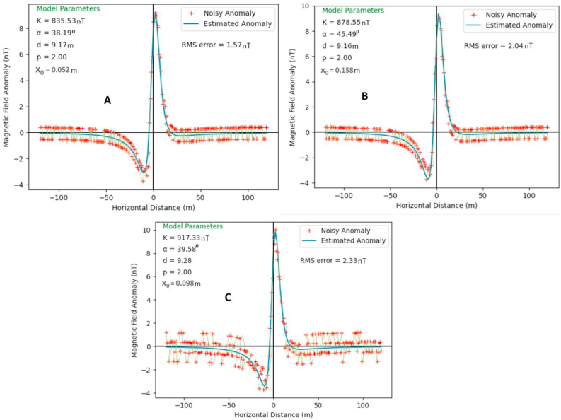
Noisy and predicted magnetic anomalies of a Thin Sheet-like geologic structure with actual model parameters of K = 800 nT, α = -20o, d = 11 m, p = 1.0, xo = 0 m with (A) 10% (B) 20% (C) 25% Gaussian noise.
Figure 11.
Change of the model parameter values with respect to the iteration number for both noiseless and noisy synthetic data sets (Spherical model) – (i) Amplitude coefficient (ii) Angle of effective magnetization (iii) depth (iv) Origin (v) Shape factor.
Figure 12.
Change of the model parameter values with respect to the iteration number for both noiseless and noisy synthetic data sets (Horizontal Cylindrical model) – (i) Amplitude coefficient (ii) Angle of effective magnetization (iii) depth (iv) Origin (v) Shape factor.
Figure 13.
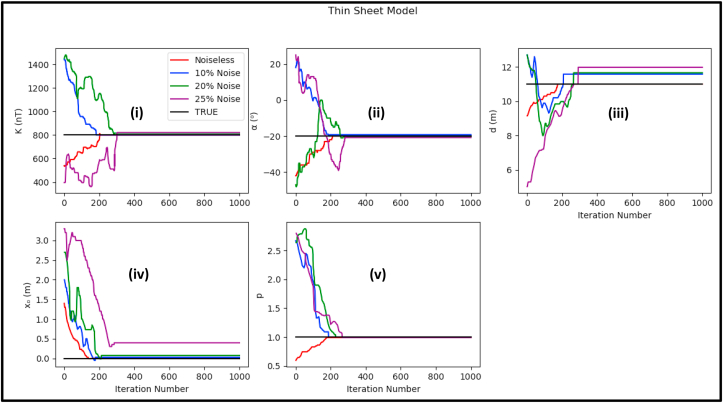
Change of the model parameter values with respect to the iteration number for both noiseless and noisy synthetic data sets (Thin sheet model) – (i) Amplitude coefficient (ii) Angle of effective magnetization (iii) depth (iv) Origin (v) Shape factor.
Figure 14.
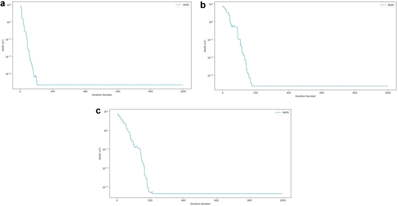
a: Convergence curve for Synthetic Anomaly (Horizontal Cylinder, 10% noise). b: Convergence curve for Synthetic Anomaly (Thin Sheet, 20% noise). c: Convergence curve for Synthetic Anomaly (Thin Sheet, 25% noise).
Figure 15.
Noisy and predicted magnetic anomalies of an infinitely long horizontal cylinder-like geologic structure with actual model parameters of K = 850 nT, α = 40o, d = 9 m, p = 2.0, xo = 0 m with (A) 10% (B) 20% (C) 25% Gaussian noise.
4. Application in modelling a multi-model case
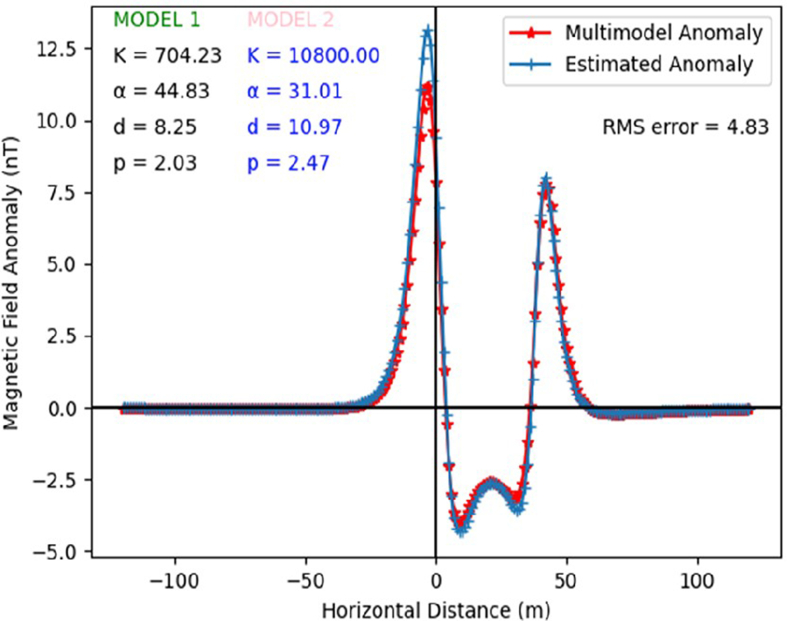
The capacity of the SSO algorithm to satisfactorily model anomalies in complicated subsurface conditions like those caused by interfering subsurface structures was tested. This was implemented by generating and modelling synthetic data from multiple sources in close proximity and with multifarious model parameters. The actual model parameters from a spherical source were K = 10,000 nT, d = 6 m, α = 30o, p = 2.5, xo = 0 m, and profile length of 120 m, while those of a horizontal cylinder had actual model parameters of K = 850 nT, d = 9 m, α = 40o, p = 2, xo = 40 m, and profile length of 120 m. The magnetic field anomaly modelled using the parameter ranges on Table 4 for this scenario is shown in Figure 16. The observed model parameters are in very good agreement with actual parameters obtained from other methods.
Table 4.
Adopted ranges of model parameters and their numerical results for the synthetic multimodal anomaly case.
| Model Parameter | Range selected | Results |
|---|---|---|
| Anomaly 1 | ||
| K (nT) | 5000–15000 | 704.23 |
| α (o) | −90–90 | 44.83 |
| d (m) | 1–15 | 8.25 |
| xo (m) | −30–30 | −3.04 |
| p | −3–5 | 2.03 |
| Anomaly 2 | ||
| K (nT) | 5000–15000 | 10800.00 |
| α (o) | −90–90 | 31.01 |
| d (m) | 1–20 | 10.97 |
| xo (m) | 0–50 | 43.05 |
| p | −3–5 | 2.47 |
Figure 16.
Synthetic and predicted magnetic anomalies from a multimodel source consisting of a sphere model with actual model parameters of K = 11,000 nT, d = 11 m, α = 30o, p = 2.5, xo = 0 m, and profile length = 120 m and horizontal cylinder actual model parameters of K = 700 nT, d = 9 m, α = 40o, p = 2, xo = 40 m and profile length of 120 m.
5. Field examples
The performance of the SSO algorithm was again tested with actual field data from ore and mineral exploration sites in order to assess its capacity to perform in such scenarios. The two field data sets were obtained from North and West Africa. The observed model parameters from these two fields were compared with results obtained from other procedures reported in literature and discussed.
Case study 1: The West Coast of Senegal Magnetic anomaly.
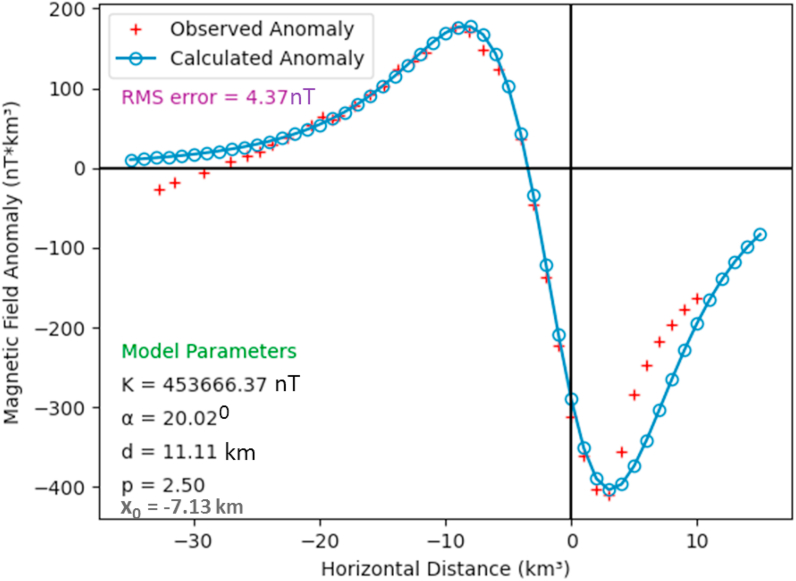
Figure 17 shows a north-south representation of a total magnetic anomaly profile from an exploration field on the West Coast of Senegal in West Africa. The causative geological body was modelled and identified by Nettleton (1976) to be a massive intrusive body within the host basement rocks. The zero crossing and the base line of the profile are as reported in Nettleton (1976) and Rao et al. (1977). The causative anomaly is characterized by a broad positive anomaly and a sharp negative anomaly on the south and north sides, respectively. For the purpose of this study, the 40 km long anomaly was digitized at 1 km interval.
Figure 17.
Magnetic inversion of the West Coast Senegal magnetic anomaly obtained using SSO procedure.
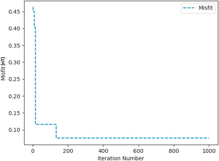
The ranges of parameter used in the inversion exercise are shown on Table 5. The SSO algorithm was used to determine the model parameters (depth, magnetic angle, amplitude coefficient, anomaly origin and shape factor) of this intrusive body. The RMS error technique was used in monitoring the misfit between the measured and those computed from the SSO procedure. The algorithm converges after 120 iterations (Figure 18) with RMS error of 4.37 nT. The modelled curve (Figure 17) and observed model parameters agree with actual model parameters (Table 5). The results show that the causative anomaly is spherically shaped with best-fitting model parameters of K = 453,666.37 nT, α = 20.02o and d = 11.11 km. These results are consistent (Table 6) with existing information about this same anomaly that are present in relevant literature (Nettleton, 1976; Prakasa Rao and Subrahmanyam, 1988; Abdelrahman et al., 2007; Mehanee et al., 2020).
Table 5.
Model parameters obtained from the inversion of magnetic anomaly from the West Coast of Senegal using SSO procedure.
| Model parameters | Selected ranges | Results | RMS error (nT) |
|---|---|---|---|
| K (nT) | 100000–700000 | 453666.37 | 4.37 |
| α (o) | −90–90 | 20.02 | |
| d (m) | 5–20 | 11.11 | |
| xo (m) | −20–10 | −7.13 | |
| p | 0–3 | 2.50 |
Figure 18.
Convergence plot for the West Coast of Senegal magnetic field anomaly case study.
Table 6.
Comparative results for the West Coast of Senegal anomaly (case study 1).
| Model parameters | Nettleton (1976) | Prakasa Rao and Subrahmanyam (1988) | Abdelrahman et al. (2007) | Mehanee et al. (2020) | Present Study |
|---|---|---|---|---|---|
| K (nT) | - | - | 310,795.00 | 461,865.90 | 453,666.37 |
| α (o) | 20.00 | 19.50 | 18.50 | 16.00 | 20.02 |
| d (m) | 10.00 | 10.80 | 11.62 | 10.00 | 11.11 |
| p | 2.50 | 2.50 | 2.50 | 2.50 | 2.50 |
Case study 2: The Hamrawein magnetic field anomaly.
The Hamrawein field is located at the western corridor bordering the Red Sea in Egypt, North Africa. In terms of oregeny, the area is an integral part of the Rift Valley System, RVS. The RVS is reported to have been formed by the anticlockwise rotation of the Arabian Tectonic Plate from the African Plate with the pole of rotation centred in the Central to Southcentral Mediterranean Sea (Noweir and Fheel, 2015). The region is characterized by meta-volcanic rocks notably pillow tholeitic basalts formed on ultramafic and gabbroic layers of substrata. These layers of strata are unconformably overlain by calcalkaline volcanic rocks and sedimentary rocks. Exhaustive details of the geology of the Hamrawein field are discussed in (Salem et al. (2005)).
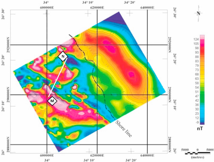
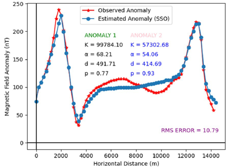
The 15 km magnetic anomaly profile was extracted from a high resolution aeromagnetic data originally acquired by Salem et al. (1999) (Figure 19). The data was digitized at 200 m interval and used for this study. The profile is characterized by two prominent anomalies at both ends (Figure 20). The anomaly is peculiar because the source of the two anomalies can be rightly or otherwise, interpreted to be from any of the simple shaped sources. The technical problem was resolved by running the SSO algorithm in a dual-combinable shape mode. The parameter ranges used in modelling this anomaly are shown on Table 7. At the end of the execution, the algorithm converges after 440 iterations (Figure 21). RMS error of 10.79 was obtained between the estimated and actual model parameters. The causative anomalies have p values of 0.77 and 0.91 for anomalies 1 and 2, respectively (Figure 20). These observations reveal that the causative anomaly is a thin sheet-like structure. The optimal model parameters were observed to be K = 99784.10 nT, d = 491.71 m, α = 68.21o and xo = 4416.84 m for the first anomaly while best fit model parameters for the second anomaly were observed to be K = 57302.68 nT, d = 414.69 m, α = 54.06o and xo = 14900.32 m (Table 7, Figure 20).
Figure 19.
Magnetic intensity map of Hamrawein magnetic field showing the profile (MN).
Figure 20.
Magnetic anomaly of Hamrawein field, Egypt inverted using the SSO procedure.
Table 7.
Numerical results for the Hamrawein magnetic field anomaly (case study 2).
| Model parameters | Selected ranges | Results |
|---|---|---|
| Anomaly 1 | ||
| K (nT) | 50000–150000 | 99784.10 |
| α (o) | 0–90 | 68.21 |
| d (m) | 100–800 | 491.71 |
| xo (m) | 1000–1000 | 4416.84 |
| p | 0–3 | 0.77 |
| Anomaly 2 | ||
| K (nT) | 10000–80000 | 57302.68 |
| α (o) | 0–90 | 54.06 |
| d (m) | 100–800 | 414.69 |
| xo (m) | 5000–20000 | 14900.32 |
| p | 0–3 | 0.91 |
Figure 21.
Convergence plot for the Hamrawein magnetic field anomaly case study.
Table 8 shows a comparison between the results obtained from SSO procedure and those obtained from other procedures published in literature. While Salem et al. (2005) interpreted the two Hamrawein Field anomalies as thin sheet structures located at depth of 555.7 and 441.2 m, Salem (2005) computed a similar shaped anomaly but reported depths of 540 and 447 m respectively for the first and second anomalies. Salem (2011) interpreted the Hamrawein Magnetic anomaly using both total gradient (TG) and local wave number (LW) methods. With the LG method, the anomaly sources were interpreted to be buried at depths of 486.5 and 440.4 m, while results from the LW technique show that the causative bodies are buried at depths of 432.6 and 422.8 m for the two anomalies. Essa and Elhussein (2018) used swarm intelligence in modelling this same data. They described the causative bodies of the anomalies to be thin sheets buried at depths of 623.05 and 494.14 m. Thus, the findings of this study obtained using the SSO procedure are in good agreement with reports obtained from previous studies.
Table 8.
Comparative results for the Hamrawein, Egypt magnetic field anomaly (case study 2).
| Model parameters | Salem et al. (2005) | Salem (2005) | Salem (2011) | Essa and Elhussein (2018) | Mehanee et al. (2020) | Present study |
|---|---|---|---|---|---|---|
| Anomaly 1 | ||||||
| K (nT) | - | - | 127595.3 | 507.64 | 102046.00 | 99784.10 |
| d (m) | 555.7 | 540.0 | 486.5 | 623.05 | 480.00 | 491.71 |
| xo (m) | 4526.0 | 4530.0 | - | 4255.98 | 4550.00 | 4416.84 |
| α (o) | - | 21.4 | - | - | 70.49 | 68.21 |
| p | 1.4 | - | 1.0 | 0.89 | 1.00 | 0.94 |
| Anomaly 2 | ||||||
| K (nT) | - | - | 83746.7 | 427.38 | 56549.52 | 57302.7 |
| d (m) | 441.2 | 477.0 | 440.4 | 494.14 | 400.00 | 414.69 |
| xo (m) | 14858.0 | 14850.0 | - | 14823.96 | 15200.00 | 14900.3 |
| α (o) | - | - | - | 37.21 | 55.04 | 54.06 |
| p | 1.2 | 1.2 | 1.0 | 0.93 | 1.00 | 0.91 |
6. Conclusion
The deployment of metaheuristic algorithms for the resolution of complex ill-posed geophysical problems is not new. In fact, these techniques have been found to be more decisive in exploring/exploiting potential solution-leading positions than their numerical counterparts. Nevertheless, even though there have been immense improvements in terms of problem resolution, some of these techniques employing metaheuristics procedures are still disarranged by flaws attributed notably to mirage-convergence, local optima, etc. These flaws, which have been found to reduce accuracy in geophysical parameter estimations, arise mostly from the way individual vectors characterizing the algorithm are strategized. In this study, the capacity and efficiency of the Social Spider Optimization algorithm in modelling distinctive body parameters (K, d, α, xo, p) of magnetic anomalies from simple geometrically-shaped (spheres, horizontal cylinders and thin sheets) causative geologic structures was investigated. Unlike previously studied heuristic algorithms where individual positions are either modified by the best-positioned individual or in some cases, a random individual concentrating population around a single particle vector (best particle); with the SSO algorithm, each individual is modelled based on their gender. This strategy promotes de-individualization of the best positioned agent allowing for the incorporation of computational mechanisms to curb/reduce the critical flaws aforementioned. The tests which were conducted on both synthetic and real (from Senegal and Egypt) magnetic anomalies with varying noise levels, were very successful. Success was based on model stability and measured for efficient performance. This includes fast and generated results for constrained multi-parameter linear problems.
The SSO procedure thereby exhibited both the fast convergence and solution accuracy. More too, uncertainty analysis conducted using the M-H sampling algorithm showed placed the geophysical parameters estimated within impressively high probability areas. These features imply a competitive processing tool, one that could easily be superior to pre-existing algorithms that are also challenged by local optima problems. Stable and efficient tool for performing geophysical data inversion.
The SSO procedure is therefore recommended for use in inverting geophysical data with higher complexities like seismic reflection and gravity data that require many corrections to be performed before reliable geological interpretations can be made. As recommendations; it is suggested that in the Case of fracture characterization from seismic data, SSO can be used to estimate Thomsen-type anisometric parameters which is widely known to define the physical characteristics of fracture networks. The algorithm can also be used to estimate velocity macro-model parameters which consist of travel-times, position and slopes of reflected events. For reservoir characterization, SSO can be used integrally with well-log data for estimation of seismic-lithologic parameters i.e porosity and permeability and acoustic impedance. For earthquake studies, optimization techniques such as Artificial Neural Network (ANN) and PSO have already been employed for the estimation of earthquake source parameters such as seismic moment and stress drop from conventional models (e.g. Model of Brune). Considering the gains of our new optimization strategy as explained in this article, SSO can comparatively improve on the process of estimating these parameters. For gravity, SSO can be adapted for the estimation of structural model parameters describing the location (such as depth origin and inclination), shape and character (such as density and amplitude) of buried features directly from gravity field data.
Declarations
Author contribution statement
Ubong C. Ben: Conceived and designed the experiments; Wrote the paper.
Anthony E. Akpan: Performed the experiments; Analyzed and interpreted the data; Wrote the paper.
Job Gideon Urang & Emmanuel I. Akaerue: Contributed reagents, materials, analysis tools or data; Wrote the paper.
Victor I. Obianwu: Analyzed and interpreted the data; Wrote the paper.
Funding statement
This research did not receive any specific grant from funding agencies in the public, commercial, or not-for-profit sectors.
Data availability statement
Data will be made available on request.
Declaration of interests statement
The authors declare no conflict of interest.
Additional information
No additional information is available for this paper.
Acknowledgements
The authors are thankful to the Management of University of Calabar for providing necessary facilities that were used for this research. We are also grateful to the anonymous reviewers for their contributions.
References
- Abdelrahman E.M., Essa K.S. A new method for depth and shape determinations from magnetic data. Pure Appl. Geophys. 2015;172:439–460. [Google Scholar]
- Abdelrahman E.M., El-Araby T.M., Soliman K.S., Essa K.S., Abo-Ezz E.R. Least-squares minimization approaches to interpret total magnetic anomalies due to spheres. Pure Appl. Geophys. 2007 [Google Scholar]
- Abdelrahman E.S.M., Abo-Ezz E.R., Essa K.S. Parametric inversion of residual magnetic anomalies due to simple geometric bodies. Explor. Geophys. 2012;43(3):178–189. [Google Scholar]
- Abo-Ezz E.R., Essa K.S. A least-squares minimization approach for model parameters estimate by using a new magnetic anomaly formula. Pure Appl. Geophys. 2016 [Google Scholar]
- Akram N., Abd-AlKareem M. Selecting best software reliability growth models: a social spider algorithm based approach. Int. J. Comput. Appl. 2018 [Google Scholar]
- Alrashidi M., Pipattanasomporn M., Rahman S. Metaheuristic optimization algorithms to estimate statistical distribution parameters for characterizing wind speeds. Renew. Energy. 2020;149:664–681. [Google Scholar]
- Alvarez J.F., Martínez J.F., Pérez C.M. Feasibility analysis of the use of binary genetic algorithms as importance samplers application to a 1-D DC resistivity inverse problem. Math. Geosci. 2008;40(4):375–408. [Google Scholar]
- Arul Xavier V.M., Annadurai S. Cluster Computing; 2019. Chaotic Social Spider Algorithm for Load Balance Aware Task Scheduling in Cloud Computing. [Google Scholar]
- Balkaya Ç., Ekinci Y.L., Göktürkler G., Turan S. 3D nonlinear inversion of magnetic anomalies caused by prismatic bodies using differential evolution algorithm. J. Appl. Geophys. 2017;136:372–386. [Google Scholar]
- Ben U.C., Ekwok E.E., Akpan A.E., Mbonu C.C., Eldosouky A.M., Abdelrahman K., Gomez-Ortiz D. Interpretation of magnetic anomalies over simple geometrical structures using Manta-Ray Foraging (MRF) Optimization. Front. Earth Sci. 2022;46(1):152–165. section Solid Earth Geophysics. [Google Scholar]
- Ben U.C., Akpan A.E., Mbonu C.C., Ebong D.E. Novel methodology for interpretation of magnetic anomalies due to two-dimensional dipping dikes using the Manta ray Foraging Optimization. J. Appl. Geophys. 2021 [Google Scholar]
- Ben U.C., Akpan A.E., Mbonu Chika H.U. Cleaner Energy and Technology; 2021. Integrated Technical Analysis of Wind Speed Data for Wind Energy Potential Assessement in Parts of Sourthern and central Nigeria. [Google Scholar]
- Ben U.C., Akpan A.E., Eze E., Awak E. Novel technique for the interpretation of gravity anomalies over geologic structures with idealized geometries using the manta ray foraging optimization. J. Asian Earth Sci. 2021 [Google Scholar]
- Bhandari A.K., Maurya S., Meena A.K. Social spider optimization based optimally weighted Otsu thresholding for image enhancement. IEEE J. Sel. Top. Appl. Earth Obs. Rem. Sens. 2018 [Google Scholar]
- Cai H., Zhdanov M. Application of Cauchy-type integrals in developing effective methods for depth-to-basement inversion of gravity and gravity gradiometry data. Geophysics. 2015;80(2) [Google Scholar]
- Cuevas E., Cienfuegos M., Zaldívar D., Pérez-Cisneros M. A swarm optimization algorithm inspired in the behavior of the social-spider. Expert Syst. Appl. 2013 [Google Scholar]
- Cuevas E., Zaldívar D., Pérez-Cisneros M. Studies in Computational Intelligence. 2018. The metaheuristic algorithm of the social-spider. [Google Scholar]
- Di Maio R., Rani P., Piegari E., Milano L. Self-potential data inversion through a Genetic-Price algorithm. Comput. Geosci. 2016 [Google Scholar]
- Ekinci Y.L., Balkaya C., Gokturkler G., Turan S. Model parameter estimations from residual gravity anomalies due to simple-shaped sources using differential evolution algorithm. J. Appl. Geophys. 2016 [Google Scholar]
- Ekinci Y.L., Özyalın S., Sındırgı P., Balkaya C., Göktürkler G. Amplitude inversion of the 2D analytic signal of magnetic anomalies through the differential evolution algorithm. J. Geophys. Eng. 2017 [Google Scholar]
- Ekinci Y.L., Balkaya C., Gokturkler G., Özyalın S. Gravity data inversion for the basement relief delineation through global optimization: a case study from the Aegean graben system, western Anatolia, Turkey. Geophys. J. Int. 2020 [Google Scholar]
- Ekinci Y.L., Yiʇitbaş E. Interpretation of gravity anomalies to delineate some structural features of Biga and Gelibolu peninsulas, and their surroundings (north-west Turkey) Geodinamica Acta. 2015;27(4) [Google Scholar]
- Ekwok S.E., Akpan A.E., Ebong E.D. Enhancement and modelling of aeromagnetic data of some inland basins, southeastern Nigeria. J. Afr. Earth Sci. 2019;155:43–53. [Google Scholar]
- Ekwok S.E., Akpan A.E., Kudamnya E.A. Exploratory mapping of structures controlling mineralization in Southeast Nigeria using high resolution airborne magnetic data. J. Afr. Earth Sci. 2020;162:103700. [Google Scholar]
- Essa K.S., Elhussein M. PSO (Particle Swarm Optimization) for interpretation of magnetic anomalies caused by simple geometrical structures. Pure Appl. Geophys. 2018;175:3539–3553. [Google Scholar]
- Essa K.S., Elhussein M. Interpretation of magnetic data through particle swarm optimization: mineral exploration cases studies. Nat. Resour. Res. 2020;29:521–537. [Google Scholar]
- Essa K.S., Elhussein M., Youssef M.A. Advances in Modeling and Interpretation in Near Surface Geophysics. Springer; Cham: 2020. Magnetic data interpretation using advanced techniques: a comparative study; pp. 263–294. [Google Scholar]
- Ewees A.A., El Aziz M.A., Elhoseny M. 8th International Conference on Computing, Communications and Networking Technologies. Vol. 2017. ICCCNT; 2017. Social-spider optimization algorithm for improving ANFIS to predict biochar yield. [Google Scholar]
- Fedi M. DEXP: a fast method to determine the depth and the structural index of potential fields sources. Geophysics. 2007 [Google Scholar]
- Fernández-Martínez J.L., García-Gonzalo E., Fernández-Álvarez J.P., Kuzma H.A., Menéndez P.O. PSO: a powerful algorithm to solve geophysical inverse problems application to a 1D-DC resistivity Case. J. Appl. Geophys. 2010;71:13–25. [Google Scholar]
- Ganguli S.S., Pal S.K., Rao J.R., Raj B.S. Gravity–magnetic appraisal at the interface of Cuddapah Basin and Nellore Schist Belt (NSB) for shallow crustal architecture and tectonic settings. J. Earth Syst. Sci. 2020;129(1):1–17. [Google Scholar]
- Gay S.P., Jr. Standard curves for interpretation of magnetic anomalies over long tabular bodies. Geophysics. 1963;28(2):161–200. [Google Scholar]
- Gobashy M., Abdelazeem M., Abdrabao M. Minerals and ore deposits exploration using meta-heuristic based optimization on magnetic data. Contrib. Geophys. Geodes. 2020 [Google Scholar]
- Göktürkler G., Balkaya Ç. Inversion of self-potential anomalies caused by simple-geometry bodies using global optimization algorithms. J. Geophys. Eng. 2012;9(5):498–507. [Google Scholar]
- Husodo A.Y., Jati G., Octavian A., Jatmiko W. IEEE Access; 2020. Enhanced Social Spider Optimization Algorithm for Increasing Performance of Multiple Pursuer Drones in Neutralizing Attacks from Multiple Evader Drones. [Google Scholar]
- Kaftan I. Interpretation of magnetic anomalies using a genetic algorithm. Acta Geophys. 2017 [Google Scholar]
- Klein C.E., Segundo E.H.V., Mariani V.C., Coelho L.D.S. Modified social-spider optimization algorithm applied to electromagnetic optimization. IEEE Trans. Magn. 2016 [Google Scholar]
- Majumder A., Das A., Das P.K. 2018. A Standard Deviation Based Firefly Algorithm for Multi-Objective Optimization of WEDM Process during Machining of Indian RAFM Steel. Neural Computing and Applications. [Google Scholar]
- Mbonu C.C., Essiett A., Ben U.C. Geospatial assessmebt of radiation hazard indices in soil samples from Njaba, Imo State, South-Eastern Nigeria. Environ. Challen. 2021;4:100117. [Google Scholar]
- Mehanee S.A. An efficient regularized inversion approach for self-potential data interpretation of ore exploration using a mix of logarithmic and non-logarithmic model parameters. Ore Geol. Rev. 2014 [Google Scholar]
- Mehanee S.A., Essa K.S. 2.5D regularized inversion for the interpretation of residual gravity data by a dipping thin sheet: numerical examples and Case studies with an insight on sensitivity and non-uniqueness. Earth Planets Space. 2015 [Google Scholar]
- Mehanee S., Essa K.S., Diab Z.E. Natural Resources Research; 2020. Imaging Depth, Structure, and Susceptibility from Magnetic Data: the Advanced Source-Parameter Imaging Method. Geophysics. [Google Scholar]
- Metropolis N., Rosenbluth A.W., Rosenbluth M.N., Teller A.H., Teller E. Equation of state calculations by fast computing machines. J. Chem. Phys. 1953;21(6):1087–1092. [Google Scholar]
- Mirjalili S., Saremi S., Mirjalili S.M., Coelho L.D.S. Multi-objective grey wolf optimizer: a novel algorithm for multi-criterion optimization. Expert Syst. Appl. 2016 [Google Scholar]
- Mosegaard K., Tarantola A. Monte Carlo sampling of solutions to inverse problems. J. Geophys. Res. Solid Earth. 1995;100(B7):12431–12447. [Google Scholar]
- Mosegaard K., Tarantola A. International Geophysics. 2002. 16 Probabilistic approach to inverse problems. [Google Scholar]
- Mota E.S.A., Medeiros W.E., Oliveira R.G. Can Euler deconvolution outline three-dimensional magnetic sources? Geophys. Prospect. 2020;68(7):2271–2291. [Google Scholar]
- Nettleton L.L. McGraw-Hill Company; 1976. Gravity and Magnetics in Oil Prospecting. [Google Scholar]
- Noweir M.A., Fheel A.S. 2015. Structural Evolution of Extensional Phanerozoic Rift Blocks: El Hamrawein Area, Northwest Red Sea, Eastern Desert, Egypt. [Google Scholar]
- Nuamah Daniel O.B., Tandoh Kingsley K. Application of 3DEuler Deconvolution and 2D inverse modelling to basin depth estimation, the Case of the Keta basin, Ghana. NRIAG J. Astron. Geophys. 2020;9(1):393–401. [Google Scholar]
- Ouadfel S., Taleb-Ahmed A. Social spiders optimization and flower pollination algorithm for multilevel image thresholding: a performance study. Expert Syst. Appl. 2016 [Google Scholar]
- Pekşen E., Yas T., Kıyak A. 1D DC resistivity modeling and interpretation in anisotropic media using particle swarm optimization. Pure Appl. Geophys. 2014;171:2371–2389. [Google Scholar]
- Pilkington M. Joint inversion of gravity and magnetic data for two-layer models. Geophysics. 2006 [Google Scholar]
- Pradhan M., Roy P.K., Pal T. Oppositional based grey wolf optimization algorithm for economic dispatch problem of power system. Ain Shams Eng. J. 2018 [Google Scholar]
- Prakasa Rao T.K.S., Subrahmanyam M. Characteristic curves for the inversion of magnetic anomalies of spherical ore bodies. Pure Appl. Geophys. PAGEOPH. 1988;126:69–83. [Google Scholar]
- Rao B.S.R., Radhakrishna Murthy I.V., Visweswara Rao C. A computer program for interpreting vertical magnetic anomalies of spheres and horizontal cylinders. Pure Appl. Geophys. PAGEOPH. 1973 [Google Scholar]
- Rao B.S.R., Rao T.K.S.P., Murthy A.S.K. A note on magnetized spheres. Geophys. Prospect. 1977 [Google Scholar]
- Rao T.P., Subrahmanyam M., Murthy A.S. Nomogram for the direct interpretation of magnetic anomalies due to long horizontal cylinders. Geophysics. 1986;51(11):2156–2159. [Google Scholar]
- Rezouki I., Boujamaoui M., Hafid M., Bba A.N., Amiri A., Inoubli M.H., et al. Contribution of gravity and aeromagnetic data to the structural modeling of the hidden faults in Guercif Basin, northeastern Morocco. J. Afr. Earth Sci. 2020;164:103797. [Google Scholar]
- Salem A. Interpretation of magnetic data using analytic signal derivatives. Geophys. Prospect. 2005;53:75–82. [Google Scholar]
- Salem A. Multi-deconvolution analysis of potential field data. J. Appl. Geophys. 2011;74:151–156. [Google Scholar]
- Salem A., Elsirafi A., Ushijima K. Memoirs of the Graduate School of Engineering, Kyushu University; 1999. Design and Application of High-Resolution Aeromagnetic Survey over Gebel Duwi Area and its Offshore Extension, Egypt. [Google Scholar]
- Salem A., Ravat D., Smith R., Ushijima K. Interpretation of magnetic data using an enhanced local wavenumber (ELW) method. Geophysics. 2005 [Google Scholar]
- Sanyi Y., Shangxu W., Nan T. Swarm intelligence optimization and its application in geophysical data inversion. Appl. Geophys. 2009;6(2):166–174. [Google Scholar]
- Scales J.A., Tenorio L. Prior information and uncertainty in inverse problems. Geophysics. 2001;66(2):389. [Google Scholar]
- Sen M.K., Stoffa P.L. second ed. Cambridge University Press; 2013. Global Optimization Methods in Geophysical Inversion. [Google Scholar]
- Sharma P.V. Magnetic method applied to mineral exploration. Ore Geol. Rev. 1987;2(1987):323–357 323. [Google Scholar]
- Shayanfar H.A., Shayeghi H., Molaee A. Proceedings of the 2016 International Conference on Artificial Intelligence, ICAI 2016 - WORLDCOMP 2016. 2016. Multi-source power system LFC using the fractional order PID controller based on SSO algorithm including redox flow batteries and SMEs. [Google Scholar]
- Snieder R. 2019. Inverse Problems in Geophysics. [Google Scholar]
- Srivastava S., Agarwal B.N.P. Inversion of the amplitude of the two-dimensional analytic signal of the magnetic anomaly by the particle swarm optimization technique. Geophys. J. Int. 2010 [Google Scholar]
- Sun H.M., Yu J.Z., Zhang X.L., Wang B.G., Jia R.S. The adaptive particle swarm optimization technique for solving microseismic source location parameters. Nonlinear Processes Geophys. 2019;26(3) [Google Scholar]
- Tarantola A. Inverse Problem Theory And Methods For Model Parameter Estimation. 2005. Inverse problem theory and methods for model parameter estimation. [Google Scholar]
- Tlas M., Asfahani J. Fair function minimization for interpretation of magnetic anomalies due to thin dikes, spheres and faults. J. Appl. Geophys. 2011 [Google Scholar]
- Tlas M., Asfahani J. The simplex algorithm for best-estimate of magnetic parameters related to simple geometric-shaped structures. Math. Geosci. 2015 [Google Scholar]
- Yu J.J.Q., Li V.O.K. A social spider algorithm for global optimization. Appl. Soft Comput. J. 2015 [Google Scholar]
- Zhdanov M.S. Geophysical inverse theory and regularization problems. Methods Geochem. Geophys. 2002 [Google Scholar]
Associated Data
This section collects any data citations, data availability statements, or supplementary materials included in this article.
Data Availability Statement
Data will be made available on request.


