Abstract
Increases in atmospheric carbon dioxide (CO2) concentrations is the main driver of global warming due to fossil fuel combustion. Satellite observations provide continuous global CO2 retrieval products, that reveal the nonuniform distributions of atmospheric CO2 concentrations. However, climate simulation studies are almost based on a globally uniform mean or latitudinally resolved CO2 concentrations assumption. In this study, we reconstructed the historical global monthly distributions of atmospheric CO2 concentrations with 1° resolution from 1850 to 2013 which are based on the historical monthly and latitudinally resolved CO2 concentrations accounting longitudinal features retrieved from fossil-fuel CO2 emissions from Carbon Dioxide Information Analysis Center. And the spatial distributions of nonuniform CO2 under Shared Socio-economic Pathways and Representative Concentration Pathways scenarios were generated based on the spatial, seasonal and interannual scales of the current CO2 concentrations from 2015 to 2150. Including the heterogenous CO2 distributions could enhance the realism of global climate modeling, to better anticipate the potential socio-economic implications, adaptation practices, and mitigation of climate change.
Subject terms: Atmospheric chemistry, Atmospheric dynamics
| Measurement(s) | atmospheric carbon dioxide concentrations |
| Technology Type(s) | satellite observations • spatial statistical analysis |
Background & Summary
Recent satellite retrievals provide a continuous global spatial products of both column CO2, e.g., from the Chinese Global Carbon Dioxide Monitoring Scientific Experimental Satellite (TanSat), the Orbiting Carbon Observatory-2 (OCO-2) and the Greenhouse Gases Observing Satellite (GOSAT); and also mid-tropospheric CO2, e.g., the atmospheric infrared sounder (AIRS), those reveal the nonuniform distributions of mid-tropospheric CO2 concentrations1–6. The satellite-derived distributions of tropospheric CO2 are generally consistent with each other, though some regional discrepancies between the satellite products have been attributed to lack of independent reference observations constraints5,7. The areas with low atmospheric CO2 concentrations are in the high latitudes and the lack of any large CO2 emissions areas1. The areas with relatively high CO2 concentrations (30°S-60°N) are formed due to high CO2 emissions from ground sources, and the horizontal and vertical movements of winds1,8. These satellite CO2 concentrations retrievals provide a potential opportunity to investigate atmospheric CO2 variability at the planetary scale.
Few climate simulation studies have been based on a globally non-uniform mean CO2 distribution patterns9–11. Those produce a bias reduction in estimated mean temperatures, and consequently some understanding of the response of Earth’s system to the actual nonuniform CO2 concentrations. In the Beijing Normal University Earth System Model (BNU-ESM), the inhomogeneous CO2 simulations are driven by annual CO2 concentrations with spatial and seasonal changes derived from satellite observation10. While in the Community Earth System Model (CESM), spatially inhomogeneous CO2 runs use prescribed gridded national-level monthly or annual CO2 emissions weighted by the grid’s population density9,11. Both BNU-ESM and CESM simulations with spatially inhomogeneous CO2 reproduce the progressive increases in temperature with better agreement with spatially distributed global surface air temperature observations than using spatially homogeneous simulations10,11. The heterogenous CO2 distributions could enhance the realism of global climate modeling.
Climate modeling taking into account the CO2 distribution could address some of the known biases in temperature in the control simulations11. Including the heterogenous CO2 distribution could enhance the realism of global climate modeling. Using BNU-ESM, global mean surface air temperature is in the inhomogeneous CO2 simulations is approximately 0.3 °C lower than that in spatially uniform runs over the period 1986–2005, reducing the warming bias seen in the uniform runs compared with the HadCRUT4 observations10. In CESM, spatially homogeneous CO2 simulations overestimated climate warming over the Arctic, tropical Pacific, while underestimated warming in the mid-latitudes, over most land areas9. The inhomogeneous runs simulated by CESM during 1950–2000 produces lower temperatures at both poles than the homogeneous runs, by up to 1.5 °C including statistically significant cooling over the Barents Sea area11.
The surface air temperature responses to spatially inhomogeneous atmospheric CO2 concentrations are mainly controlled by changes in large scale atmospheric circulations, e.g., the Hadley cell, westerly jet, Arctic Oscillation and Rossby waves8–11. Local surface air temperature anomalies under nonuniform CO2 simulations are affected by the CO2 physiological response over vegetated areas. The land plants adjust to changes in atmospheric CO2 by altering their stomatal conductance, which consequently affects the water evapotranspiration from plant leaf to atmosphere12. This affects environmental temperature through evaporative cooling, and the evaporated moisture alters the air humidity and influences low cloud amounts by the water vapor diffusion, which is especially obvious in summer when the plants grow vigorously. In the polar areas, the degree of warming amplification depends strongly on the locally distribution of CO2 radiative forcing, specifically through positive local lapse-rate feedback, with ice-albedo and Planck feedbacks playing subsidiary roles, also suggesting that inhomogeneous spatial distributions of CO2 concentrations is consistent with significant climatic effects13. In marine ecosystems, non-uniform atmospheric CO2 and temperature biases could affect the uptake and storage of CO2 in the ocean, which will change regional atmospheric CO2 concentrations, ocean pH, ocean oxygen concentrations and primary production14.
Existing studies with spatially homogeneous atmospheric CO2 concentrations may have underestimated the temperature gradient from mid-latitudes to high latitudes. Some atmospheric circulation patterns, e.g., the Hadley cell, westerly jet and Arctic Oscillation are theoretically related to the mid- to high-latitude temperature gradients, and are hence potentially incorrectly simulated9. Spatially homogeneous atmospheric CO2 simulations underestimate interannual variability in regional temperature and precipitation relative to the inhomogeneous simulations9 and so can result in underrating magnitudes and frequencies of extreme event such as droughts, heat waves, floods, and hurricanes12. The upper 3 m of Arctic permafrost holding twice as much carbon as the atmosphere is accelerating its thaw due to the intensification of Arctic warming, leading to Greenhouse gases release and accelerating global warming15. Biases of temperature from spatially uniform CO2 responses to ice-albedo-temperature feedbacks would lead to overestimated polar warming relative to inhomogeneously distributed CO2 in the historical period13.
However, climate simulation studies are almost based on a globally uniform mean CO2 or latitudinally resolved CO2 datasets for the historical and future scenarios in the Climate Model Intercomparison Project16–19. In the models including representation of the carbon cycle, the CMIP simulations can be driven by prescribed CO2 emissions accounting explicitly for fossil fuel combustion19. Feng et al.20 provided spatially distributed anthropogenic emissions historical data with annual resolution and future scenario data in 10-year intervals for CMIP6. There is near-real-time daily CO2 emission dataset monitoring the variations in CO2 emissions from fossil fuel combustion and cement production since January 1, 2019 at the national level21. Shan et al.22 constructed the time-series of CO2 emission inventories for China and its 30 provinces following the Intergovernmental Panel on Climate Change (IPCC) emissions accounting method with a territorial administrative scope. The other CMIP simulations can be driven by prescribed CO2 concentrations, which enables these more complex models to be evaluated fairly against those models without representation of carbon cycle processes19. Meinshausen et al.17 provided a prescribed global-mean greenhouse gases (GHGs) concentrations using atmospheric concentration observations and emissions estimates in the historical period (1750–2005) and using four different Integrated Assessment Models in the future scenario, with some models constraining internally generated fields of GHG concentrations to match those global-mean values. For CMIP6, Meinshausen et al.18 updated those global-mean and latitudinal monthly-resolved GHG concentration dataset in the historical period. In the future period, there are global annual mean GHG concentration dataset in some alternative scenarios of future emissions and land use changes produced with integrated assessment models19.
Here, we provide global monthly distributions of atmospheric CO2 concentrations with 1° resolution under historical (1850–2013) and future (2015–2150) scenarios in CMIP6, which have equal global annual mean values in the CMIP6 standard CO2 dataset. The monthly CO2 distributions dataset can be accessed by the Zenodo data repository23 (10.5281/zenodo.5021361). Climate modeling taking into account heterogenous CO2 distributions could reduce some of the known biases in the control simulations9–11, to better anticipate the potential socio-economic implications, adaptation practices, and mitigation of climate change.
Methods
The historical CO2 concentrations follows CMIP6 monthly and latitudinally resolved CO2 concentrations accounting longitudinal features retrieved from fossil-fuel CO2 emissions from Carbon Dioxide Information Analysis Center. And the spatial distributions of CO2 under SSP-RCPs scenarios were generated based on the spatial, seasonal and interannual features of the current CO2 concentrations distributions.
Historical CO2 concentrations spatial reconstruction
Since lack of observational evidence of both seasonality and latitudinal gradients of CO2 concentrations in pre-industrial times, CMIP6 project provides consolidated dataset of historical atmospheric concentrations of CO2 based on the Advanced Global Atmospheric Gases Experiment (AGAGE) and National Oceanic and Atmospheric Administration (NOAA) networks, firn and ice core data, and archived air data, and a large set of published studies for the earth system modeling experiments18. The dataset provides best-guess estimates of historical forcings with latitudinal and seasonal features (available at https://www.climatecollege.unimelb.edu.au/cmip6).
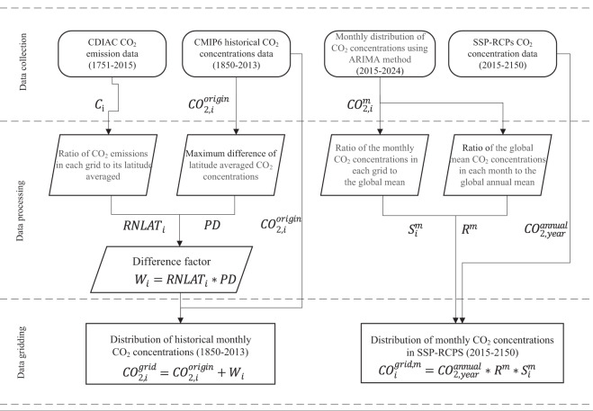
The atmospheric CO2 concentrations from CMIP6 has only spatial distributions in latitude but not in longitude. We reconstructed the CMIP6 historical CO2 concentration data with global 1° resolution based on the fossil-fuel CO2 emissions data from Carbon Dioxide Information Analysis Centre (CDIAC). The CDIAC fossil-fuel CO2 emissions used here are based on fossil-fuel consumption estimates, which distributes spatially on a 1° latitude by 1° longitude grid from 1751 to 201324. (available at https://cdiac.ess-dive.lbl.gov/trends/emis/meth_reg.html). However, there is no value of the CDIAC CO2 emissions over land without human activity and ocean, where CO2 emissions values are filled with the average values of their latitudes of CO2 emissions. The processed global carbon emissions data from CDIAC is used as features of CO2 distributions and seasonal cycle for downscaling historical atmospheric CO2 concentrations in each month (Fig. 1). The ratio of CDIAC CO2 emissions in each grid to its latitude averaged is calculated as:
| 1 |
where Ci represents CO2 emission in each grid, and CLAT is the corresponding latitude average CO2 emissions.
Fig. 1.
The processes for CO2 concentrations distributions reconstruction in the historical period and future scenarios.
The ratio RLATi is normalized as,
| 2 |
where represents the normalized ratio RLATi, is the maximum value of RLATi, and is the minimum value of RLATi.
The maximum difference of latitude averaged CO2 concentrations (PD) for CMIP6 data is calculated as,
| 3 |
where is the maximum latitude CO2 concentration, represents the minimum latitude CO2 concentration.
The difference factor in each grid is calculated as,
| 4 |
The reconstructed CO2 concentrations equals to original CO2 concentrations and the difference factor in each grid, as
| 5 |
where is the CO2 concentrations in CMIP6.
SSP-RCPs CO2 concentrations spatial reconstruction
In the future time period, CO2 concentration data for CMIP6 from 2015 were derived from the eight shared socioeconomic pathway (SSP) and representative concentration pathways (RCP) scenarios (Table 1) using the reduced-complexity climate–carbon-cycle model MAGICC7.025. The five SSP scenarios SSP1-1.9, SSP1-2.6, SSP2-4.5, SSP3-7.0, and SSP5-8.5 that are used as priority scenarios highlighted in ScenarioMIP for the IPCC sixth assessment report19. The SSP1-1.9 and SSP1-2.6 are both in the “sustainability” SSP1 socio-economic pathway but with about 1.9 and 2.6 W m−2 radiative forcing level in 2100, reflecting ways for 1.5°C and 2°C targets under the Paris Agreement, respectively. The SSP2-4.5 follows “middle of the road” socio-economic pathway with a nominal 4.5 W m−2 radiative forcing level by 2100. The SSP3-7.0 is in the “regional rivalry” socio-economic pathway and a medium-high radiative forcing scenario. SSP5-8.5 marks the upper edge of the SSP scenario spectrum with a high reference scenario in a high fossil fuel development world throughout the 21st century. SSP5-3.4 follows SSP5-8.5, an unmitigated baseline scenario, through 2040, at which point aggressive mitigation is undertaken to rapidly reduce emissions to zero by about 2070 and to net negative levels thereafter. In addition, the SSP4-6.0 and SSP4-3.4 scenarios update the RCP6.0 pathway and fill a gap at the low end of the range of future forcing pathways, respectively. CMIP6 CO2 concentration data in each SSP-RCP scenario is available at https://esgf-node.llnl.gov/search/input4mips/.
Table 1.
Summary for experimental scenarios designed in ScenarioMIP19.
| Scenario name | SSP category | Forcing category | 2100 forcing (W m−2) |
|---|---|---|---|
| SSP1-1.9 | Sustainability | Low | 1.9 |
| SSP1-2.6 | Sustainability | Low | 2.6 |
| SSP2-4.5 | Middle of the road | Medium | 4.5 |
| SSP3-7.0 | Regional rivalry | High | 7.0 |
| SSP4-3.4 | Inequality | Low | 3.4 |
| SSP4-6.0 | Inequality | Medium | 6.0 |
| SSP5-3.4 | Fossil-fueled development | Low | 3.4 |
| SSP5-8.5 | Fossil-fueled development | High | 8.5 |
The global annual mean atmospheric CO2 in the CMIP6 future scenarios are interpolated temporally and spatially based on the features of CO2 distributions and seasonal cycle of the current monthly atmospheric CO2 concentrations distributions from 2015 to 2024 (the geotif2nc_2015_2024.nc file is contained within “Code.zip” archive accessed via the Zenodo data repository23 10.5281/zenodo.5021361) simulated based on the monthly reconstructed historical CO2 concentrations using autoregressive integrated moving average (ARIMA) method26,27 (Fig. 1).
The ratio () of the monthly CO2 concentrations in each grid to the global mean averaged during 2015–2024 is calculated as
| 6 |
where is the monthly CO2 concentrations in each month m (m = 1, 2…12) and in each grid i. is the global mean CO2 concentrations in each month m.
The ratio () of the global mean CO2 concentrations in each month to the global annual mean averaged during 2015–2024 is calculated as,
| 7 |
where is the global annual mean CO2 concentration averaged during 2015–2024.
The CO2 concentrations distributions in each year are obtained by
| 8 |
where is the global annual mean CO2 concentrations in the CMIP6 future scenarios.
Data Records
All atmospheric CO2 output grids can be accessed via the Zenodo data repository23 (10.5281/zenodo.5021361). The data records include 1 file Network Common Data Form (NetCDF) format for CO2 distributions in historical period named CO2_1deg_month_1850–2013.nc, and 8 files NetCDF format with the naming convention CO2_SSP{XYY}_2015_2150.nc, where X and YY are the shared socioeconomic pathway and radiative forcing level at 2100, respectively, for CO2 distributions in the future scenarios. Each NetCDF file includes 3 dimensions: time (month of the year expressed as days since the first day of 1850, n = 1968 and 1632 for the historical and the future, respectively); latitude (Degrees North of the equator [cell centres], n = 180); longitude (Degrees East of the Prime Meridian [cell centres], n = 360). Each NetCDF file contains a monthly variable representing mole fraction of carbon dioxide in air (variable name: values in the historical file and in the future scenario files) with the unit ppm and the 1° × 1° resolution. There are 127,526,400 and 105, 753,600 unique data points for the historical file and each future scenario file. All grids are bottom-left arranged with coordinates referenced to the prime meridian and the equator.
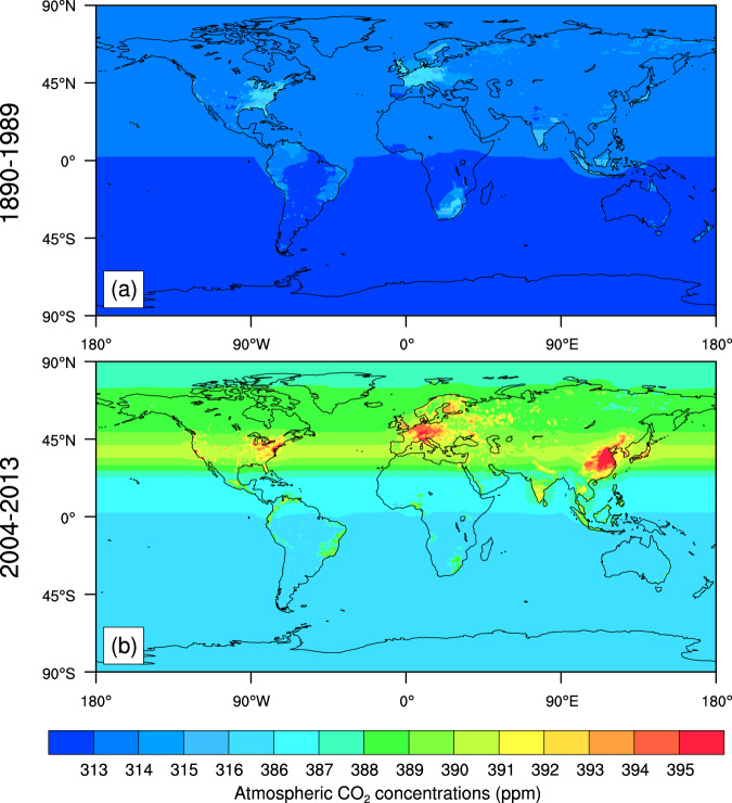
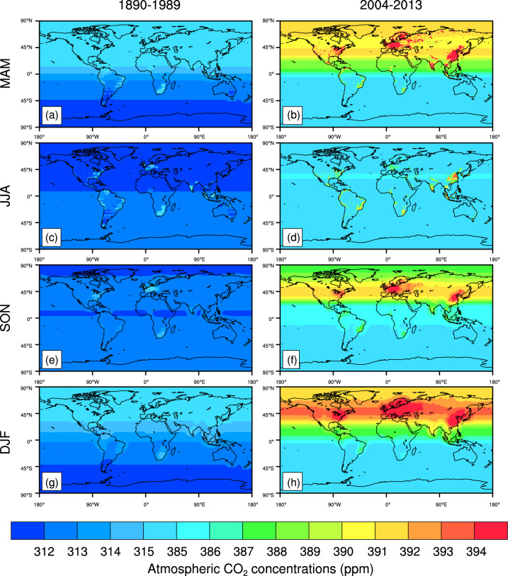
The spatial distributions of historical CO2 concentrations averaged during 1890–1989 shows that the high CO2 concentrations appears in the developed regions, e.g., Europe and Eastern part of the United States (Fig. 2). CO2 concentrations in the United Kingdom and the United States are 290.90 ppm and 287.83 ppm, respectively, during 1861–1880 (Table 2). During 2004–2013, the average CO2 concentrations in the United Kingdom and the United States increase to 391.65 ppm and 389.99 ppm, respectively (Table 2), which are associated with regional CO2 emissions. In addition, the CO2 concentration 391.16 ppm in China is slightly less than that in the United Kingdom, which is associated with the low CO2 concentrations in the west of China (Fig. 2). Fig. 3 shows the distributions of seasonal atmospheric CO2 concentrations (ppm) in these seasons March-April-May (MAM), June-July-August (JJA), September-October-November (SON), and December-January-February (DJF).
Fig. 2.
The maps of global historical atmospheric CO2 concentrations (ppm) averaged during 1890–1989 (Top) and averaged during 2004–2013 (Bottom).
Table 2.
Multi-year average atmospheric CO2 concentrations in various historical periods for some countries.
| Regional CO2 concentrations (ppm) | 1861–1880 | 1901–1920 | 1941–1960 | 1981–2000 | 2004–2013 |
|---|---|---|---|---|---|
| Australia | 287.83 | 299.66 | 313.07 | 353.11 | 384.32 |
| Brazil | 287.53 | 299.79 | 313.66 | 354.54 | 385.71 |
| Canada | 287.59 | 300.12 | 314.04 | 355.73 | 388.46 |
| China | 287.60 | 300.04 | 313.87 | 356.59 | 391.16 |
| India | 287.57 | 300.52 | 314.55 | 356.56 | 389.25 |
| United States | 287.83 | 300.8 | 314.61 | 356.25 | 389.99 |
| United Kingdom | 290.90 | 303.38 | 317.29 | 358.73 | 391.65 |
Fig. 3.
The maps of seasonal atmospheric CO2 concentrations (ppm) averaged during 1890–1989 (a) and averaged during 2004–2013 (b) in these March-April-May (MAM), June-July-August (JJA), September-October-November (SON), and December-January-February (DJF).
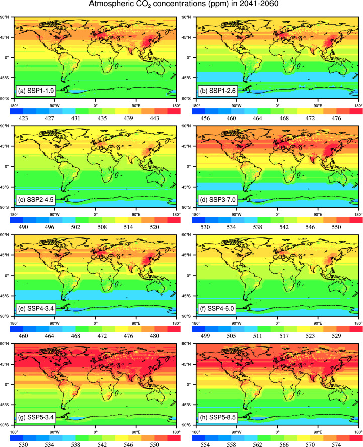
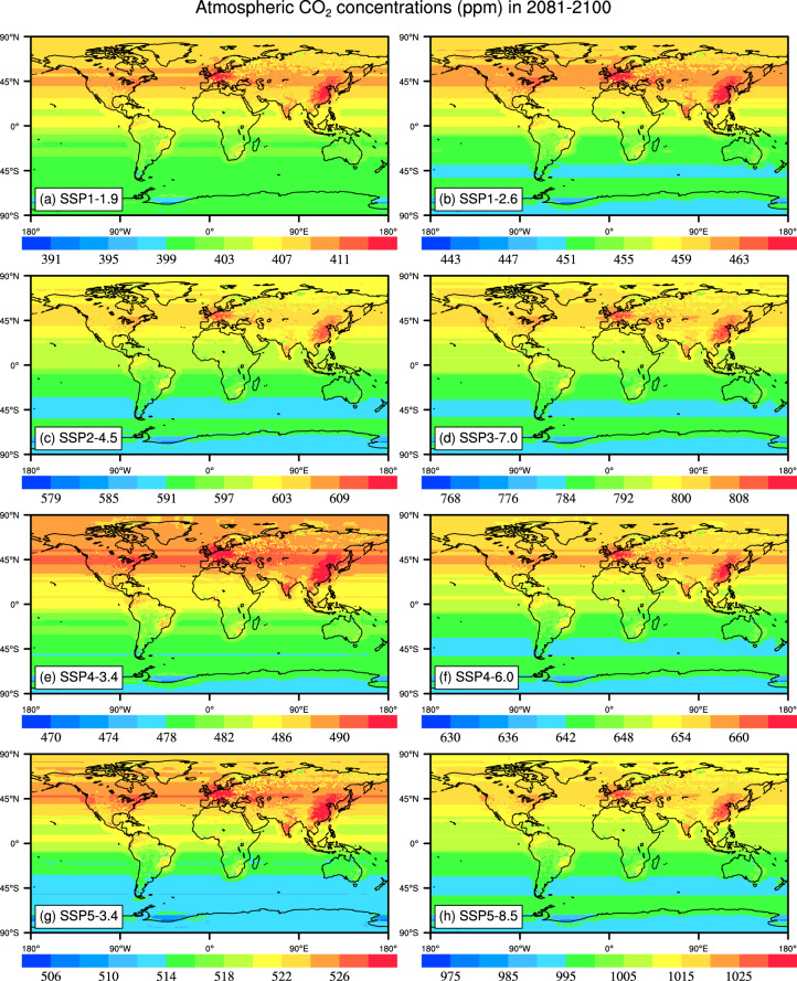
CO2_SSP{XYY}_2015_2150.nc files are generated based on the eight SSP and RCP scenarios, including SSP1-1.9, SSP1-2.6, SSP2-4.5, SSP3-7.0, SSP4-3.4, SSP4-6.0, SSP5-3.4 and SSP5-8.5 which provide global distributions of CO2 concentrations under different socio-economic development pathway associated radiative forcing levels. In these eight scenarios, the average CO2 concentrations in the Northern Hemisphere (NH) is higher than that in the Southern Hemisphere (SH). High CO2 concentrations relative to the global average is mainly distributed in Europe, Eastern United States, and East Asia. Under each scenario, global CO2 concentrations averaged in 2041-2060 ranges 420–590 ppm, and the CO2 concentrations averaged during 2081–2100 is between 380–1030 ppm (Figs. 4, 5). Under SSP5-8.5, the average CO2 concentrations in China and the United Kingdom are 1020.70 ppm and 1021.51 ppm, respectively, during 2081–2100, while the CO2 concentration is 998.28 ppm in Australia (Table 3).
Fig. 4.
The maps of global atmospheric CO2 concentrations (ppm) averaged during 2041–2060 in the SSP1-1.9, SSP1-2.6, SSP2-4.5, SSP3-7.0, SSP4-3.4, SSP4-6.0, SSP5-3.4 and SSP5-8.5 scenarios. The period of 2041–2060 selected is for the average state in the middle of this century, the key time for carbon neutrality.
Fig. 5.
The maps of global atmospheric CO2 concentrations (ppm) averaged during 2081–2100 in the SSP1-1.9, SSP1-2.6, SSP2-4.5, SSP3-7.0, SSP4-3.4, SSP4-6.0, SSP5-3.4 and SSP5-8.5 scenarios. The period of 2081–2100 in the Fig. 5 chosen is for the average state at the end of this century.
Table 3.
Multi-year average atmospheric CO2 concentrations between 2081–2100 in some countries under future scenarios.
| Regional CO2 concentrations during 2081–2100 (ppm) | SSP1-1.9 | SSP1-2.6 | SSP2-4.5 | SSP3-7.0 | SSP4-3.4 | SSP4-6.0 | SSP5-3.4 | SSP5-8.5 |
|---|---|---|---|---|---|---|---|---|
| Australia | 401.47 | 452.88 | 592.52 | 786.85 | 480.57 | 644.23 | 514.99 | 998.28 |
| Brazil | 404.42 | 456.21 | 596.88 | 792.64 | 484.11 | 648.98 | 518.78 | 1005.63 |
| Canada | 408.62 | 460.95 | 603.07 | 800.87 | 489.13 | 655.71 | 524.16 | 1016.06 |
| China | 410.48 | 463.05 | 605.82 | 804.52 | 491.36 | 658.70 | 526.56 | 1020.70 |
| India | 408.62 | 460.95 | 603.08 | 800.88 | 489.13 | 655.72 | 524.17 | 1016.07 |
| United States | 409.14 | 461.54 | 603.85 | 801.90 | 489.76 | 656.55 | 524.84 | 1017.37 |
| United Kingdom | 410.81 | 463.42 | 606.31 | 805.17 | 491.75 | 659.23 | 526.98 | 1021.51 |
Technical Validation
In this validation section, GOSAT surface CO2 concentrations and AIRS mid-tropospheric CO2 concentrations products were used for comparison with the reconstructed distributions of atmospheric CO2 concentrations. The GOSAT launched in January 2009 observing infrared light reflected and emitted from the earth’s surface and the atmosphere provides three-dimensional distributions of CO2 products calculated from the Level 4 A data product using a global atmospheric transport model from 200928–30. The data product has a horizontal resolution of 2.5° × 2.5° and a time step of six hours. The satellite Aqua was launched in May 2002 and operates in a near polar sun-synchronous orbit, and its mission is to observe the global water and energy cycle, climate change trend, and response of the climate system to the increase in greenhouse gases1,31. It retrieves the global daily or monthly CO2 concentrations over land, ocean and polar regions6. AIRS mid-tropospheric CO2 concentrations product is retrieved using the Vanishing Partial Derivative method32, with the 90 km × 90 km spatial resolution covering 90°N–60°S. The AIRS CO2 retrieval product provides a continuous global nonuniform distributions of mid-tropospheric CO2 concentrations from 2003 to 2016.
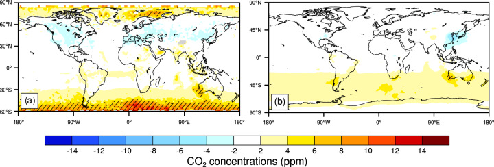
The multi-year mean reconstructed atmospheric CO2 concentrations are slightly higher than that of the AIRS mid-tropospheric CO2 concentrations product in the NH high latitudes and mid-latitudes of the SH, but lower in the mid-latitudes of the SH. In the 45°S-60°S latitude band, about 10 ppm (3%) increase in the reconstructed CO2 concentrations is statistically significant relative to the AIRS averaged during 2003–2016 (Fig. 6a). The reconstructed CO2 concentrations are about 4 ppm (1%) higher and lower than the GOSAT surface CO2 concentrations in the 30°S-60°S latitude band and in the East Asia and its adjacent sea areas, respectively, however, the biases are both not statistically significant at the 5% level using the Student’s t test (Fig. 6b).
Fig. 6.
Changes in CO2 concentrations (ppm) between the reconstructed and AIRS (a) averaged during 2003–2016 (excluding 2014), and between the reconstructed and GOSAT (b) averaged during 2010–2018 (excluding 2014). The time periods selected are decided by data available. Hatched areas are regions where changes are statistically significant at the 5% level using the Student’s t test.
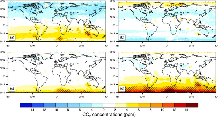
Relative to the AIRS, there are some statistically significant seasonal overestimations of the reconstructed CO2 concentrations with over 12 ppm averaged during 2003–2016 mainly located in the 45°S–60°S latitude band in DJF (Fig. 7). In MAM, the reconstructed CO2 concentrations are 2-6 ppm lower in the NH and 2-6 ppm higher in the SH than that in the AIRS. In JJA, the reconstructed CO2 concentrations are 2-6 ppm lower at the latitude bands of 30°N–60°N, 15°S–30°S, and 45°S–60°S, and 2-6 ppm higher in the 60°N–90°N latitude band than that in the AIRS. In SON, the bias of the reconstructed CO2 concentrations is from −2 to 2 ppm in most regions of the world, except in 45°S-60°S latitude band relative to the AIRS.
Fig. 7.
Changes in the seasonal (a, MAM; b, JJA; c, SON; d, DJF) CO2 concentrations (ppm) between the reconstructed and the AIRS product averaged during 2003–2016 (excluding 2014). The time period selected is decided by data available. Hatched areas are regions where changes are statistically significant at the 5% level using the Student’s t test.
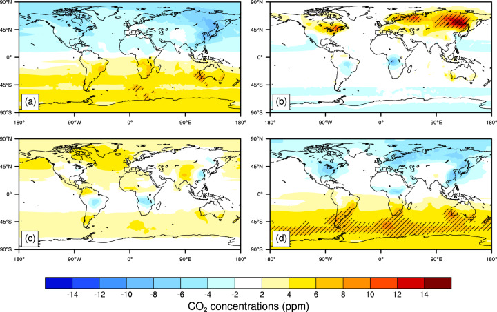
Relative to the GOSAT, there are some statistically significant seasonal overestimations of the reconstructed CO2 concentrations between 8 to 10 ppm averaged during 2010–2018 mainly at the 45°S-70°S latitude bands in DJF (Fig. 8). In JJA, the reconstructed CO2 concentrations are over 10 ppm higher than the GOSAT data in the Far eastern and North-western federal districts of Russia, and Eastern Canada. In MAM, the reconstructed CO2 concentrations are 2-8 ppm lower in the NH and 2-6 ppm higher in the SH than that in the GOSAT. In SON, the overestimations of the reconstructed CO2 concentrations are from 2 to 6 ppm, and the underestimations of the reconstructed CO2 concentrations is from −6 to −2 ppm in some areas of South America, South Africa and Eastern China relative to the GOSAT.
Fig. 8.
Changes in the seasonal (a, MAM; b, JJA; c, SON; d, DJF) CO2 concentrations (ppm) between the reconstructed and the GOSAT product averaged during 2010–2018 (excluding 2014). The time period selected is decided by data available. Hatched areas are regions where changes are statistically significant at the 5% level using the Student’s t test.
Compared with the GOSAT surface atmospheric CO2 concentrations, there is similar trend and seasonal cycles with the monthly global mean reconstructed CO2 concentrations (Fig. 9a). The seasonal cycle with high CO2 concentrations in MAM and low CO2 concentrations in JJA is closely related to the seasonal cycle of plant growth33. The monthly global mean AIRS mid-tropospheric CO2 concentrations have a similar trend and the peak feature of each seasonal cycle with the reconstructed and GOSAT CO2 concentrations, but the valley feature of seasonal cycles, which is associated with the transport of atmospheric CO2 and less impacts from plant CO2 absorption34,35. The R-squared correlation (R2) is 0.95 between the monthly global mean reconstructed CO2 and the AIRS CO2 product, and the R2 between the reconstructed and the GOSAT product is 0.99 (Fig. 9b).
Fig. 9.
Monthly global mean time evolution of CO2 concentrations (ppm) for the AIRS (red, from Jan 2003 to Feb 2017), the GOSAT (blue, from Jun 2009 to oct 2017), and the reconstructed data (cyan) from 2003 to 2017 (a); and scatter plot between the monthly global mean reconstructed data, and the AIRS (red) and the GOSAT (blue), respectively averaged during 2010–2016 (b). The reconstructed CO2 data from 2010–2013 and 2015–2017 compared here is from the historical and the SSP5-8.5 reconstructions, respectively.
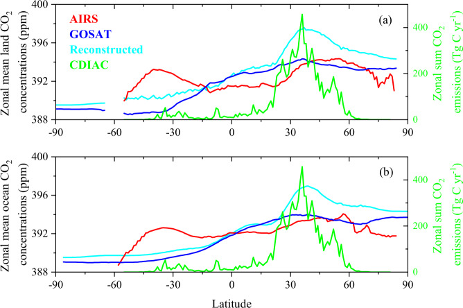
Figure 10 shows the zonal mean CO2 concentrations (ppm) for the AIRS, the GOSAT, and the reconstructed data during 2010 to 2013 averaged over land and averaged over ocean, separately. The zonal mean CO2 concentrations for the reconstructed data averaged over land and over ocean both have a similar distribution pattern with the surface CO2 concentrations in GOSAT, with higher CO2 values in the Northern Hemisphere than that in the Southern Hemisphere, though there are some overestimates in the middle latitudes for the reconstructed CO2 concentrations, which is consistent with the high CO2 emissions in the middle latitude bands (Fig. 10). In the low and middle latitudes of the Southern Hemisphere, the reconstructed CO2 concentrations over land and over ocean are both between the AIRS and the GOSAT range of CO2 concentrations, respectively (Fig. 10). We also note that our historical CO2 concentrations distributions should be regarded as highly uncertain. However, some plausibility of the CO2 concentrations distributions is obtained by comparison with satellite observations (e.g., ARIS, GOSAT satellite CO2 concentrations products) at the zonal mean and grid scales.
Fig. 10.
Zonal mean CO2 concentrations (ppm) averaged over land (a) and over ocean (b) for the AIRS, the GOSAT, and the reconstructed data during 2010 to 2013. Zonal sum fossil-fuel CO2 emissions (Tg C yr−1) are also showed using the right y axis in each panel from Carbon Dioxide Information Analysis Center (CDIAC) averaged during 2010 to 2013.
Usage Notes
This data is intended for use as a prior in global climate modeling, potential socio-economic implications and mitigation of climate change, and adaptation practices. The historical global monthly distributions of atmospheric CO2 concentrations with 1° resolution from 1850 to 2013, including 1 file NetCDF format file named CO2_1deg_month_1850-2013.nc And the spatial distributions of nonuniform CO2 under SSP-RCP scenarios are from 2015 to 2150, including 8 files NetCDF format with the naming convention CO2_SSP{XYY}_2015_2150.nc, where X and YY are the shared socioeconomic pathway and radiative forcing level at 2100, respectively. Each NetCDF file contains a monthly variable representing mole fraction of carbon dioxide in air (ppm). including 3 dimensions: time (month of the year expressed as days since the first day of 1850, n = 1968 and 1632 for the historical and the future, respectively); latitude (Degrees North of the equator [cell centres], n = 180); longitude (Degrees East of the Prime Meridian [cell centres], n = 360). We anticipate that the dataset will be widely used by Earth system modeling, agriculture management, and socio-economic analysis, to assess the climate, environmental and socio-economic implications of considering past and on-going inhomogeneous CO2 distributions, and for formulating strategies of spatial, as well as global carbon reduction.
Acknowledgements
This research was supported by the National Key Research and Development Program of China (Grant No. 2016YFA0602500). Data production and technical validation were partially funded by the Strategic Priority Research Program of Chinese Academy of Sciences (Grant No. XDA23070400) and the state key program of National Natural Science Foundation of China (Grant No. 91425303; Grant No. 71533004).
Author contributions
X.D. and L.D. led the project, W.C., Y.W., J.P., J.T., S.J., H.Z. and X.W. drafted the manuscript, X.D., L.D., J.F., Z.L., X.Z., D.Z. and W.Q. revised the manuscript.
Code availability
The code used to perform all steps described here and shown in Fig. 1 is contained within a.zip archive named “Code.zip”. The code can be accessed via the Zenodo data repository23 (10.5281/zenodo.5021361).
Competing interests
The authors declare no competing interests.
Footnotes
Publisher’s note Springer Nature remains neutral with regard to jurisdictional claims in published maps and institutional affiliations.
Contributor Information
Li Dan, Email: danli@tea.ac.cn.
Xiangzheng Deng, Email: dengxz@igsnrr.ac.cn.
Yongli Wang, Email: wangyl@tea.ac.cn.
Jing Tian, Email: tianj.04b@igsnrr.ac.cn.
References
- 1.Cao L, et al. The Global Spatiotemporal Distribution of the Mid-Tropospheric CO2 Concentration and Analysis of the Controlling Factors. Remote Sens. 2019;11:94. doi: 10.3390/rs11010094. [DOI] [Google Scholar]
- 2.Lei L, et al. A comparison of atmospheric CO2 concentration GOSAT-based observations and model simulations. Sci. China-Earth Sci. 2014;57:1393–1402. doi: 10.1007/s11430-013-4807-y. [DOI] [Google Scholar]
- 3.Kuang Z, Margolis J, Toon G, Crisp D, Yung Y. Spaceborne measurements of atmospheric CO2 by high-resolution NIR spectrometry of reflected sunlight: An introductory study. Geophys. Res. Lett. 2002;29:11-1–11–4. doi: 10.1029/2001GL014298. [DOI] [Google Scholar]
- 4.Kuze A, Suto H, Nakajima M, Hamazaki T. Thermal and near infrared sensor for carbon observation Fourier-transform spectrometer on the Greenhouse Gases Observing Satellite for greenhouse gases monitoring. Appl. Optics. 2009;48:6716–6733. doi: 10.1364/AO.48.006716. [DOI] [PubMed] [Google Scholar]
- 5.Yang D, et al. The First Global Carbon Dioxide Flux Map Derived from TanSat Measurements. Adv. Atmos. Sci. 2021;38:1433–1443. doi: 10.1007/s00376-021-1179-7. [DOI] [Google Scholar]
- 6.Chahine, M. T. et al. Satellite remote sounding of mid-tropospheric CO2. Geophys. Res. Lett. 35 (2008).
- 7.Wang T, Shi J, Jing Y, Xie Y. Investigation of the consistency of atmospheric CO2 retrievals from different space-based sensors: Intercomparison and spatiotemporal analysis. Chin. Sci. Bull. 2013;58:4161–4170. doi: 10.1007/s11434-013-5996-7. [DOI] [Google Scholar]
- 8.Ying N, et al. Rossby Waves Detection in the CO2 and Temperature Multilayer Climate Network. Geophys. Res. Lett. 2020;47:e2019GL086507. doi: 10.1029/2019GL086507. [DOI] [Google Scholar]
- 9.Zhang X, Li X, Chen D, Cui H, Ge Q. Overestimated climate warming and climate variability due to spatially homogeneous CO2 in climate modeling over the Northern Hemisphere since the mid-19 th century. Sci Rep. 2019;9:1–9. doi: 10.1038/s41598-019-53513-7. [DOI] [PMC free article] [PubMed] [Google Scholar]
- 10.Wang Y, Feng J, Dan L, Lin S, Tian J. The impact of uniform and nonuniform CO2 concentrations on global climatic change. Theor. Appl. Climatol. 2020;139:45–55. doi: 10.1007/s00704-019-02924-7. [DOI] [Google Scholar]
- 11.Navarro A, Moreno R, Tapiador FJ. Improving the representation of anthropogenic CO2 emissions in climate models: impact of a new parameterization for the Community Earth System Model (CESM) Earth Syst. Dynam. 2018;9:1045–1062. doi: 10.5194/esd-9-1045-2018. [DOI] [Google Scholar]
- 12.Skinner CB, Poulsen CJ, Mankin JS. Amplification of heat extremes by plant CO2 physiological forcing. Nat. Commun. 2018;9:1094. doi: 10.1038/s41467-018-03472-w. [DOI] [PMC free article] [PubMed] [Google Scholar]
- 13.Stuecker MF, et al. Polar amplification dominated by local forcing and feedbacks. Nat. Clim. Chang. 2018;8:1076–1081. doi: 10.1038/s41558-018-0339-y. [DOI] [Google Scholar]
- 14.Nagelkerken I, Connell SD. Global alteration of ocean ecosystem functioning due to increasing human CO2 emissions. Proc. Natl. Acad. Sci. USA. 2015;112:13272–13277. doi: 10.1073/pnas.1510856112. [DOI] [PMC free article] [PubMed] [Google Scholar]
- 15.Turetsky MR, et al. Permafrost collapse is accelerating carbon release. Nature. 2019;569:32–34. doi: 10.1038/d41586-019-01313-4. [DOI] [PubMed] [Google Scholar]
- 16.Taylor KE, Stouffer RJ, Meehl GA. An Overview of CMIP5 and the Experiment Design. Bull. Amer. Meteorol. Soc. 2012;93:485–498. doi: 10.1175/BAMS-D-11-00094.1. [DOI] [Google Scholar]
- 17.Meinshausen M, et al. The RCP greenhouse gas concentrations and their extensions from 1765 to 2300. Clim. Change. 2011;109:213. doi: 10.1007/s10584-011-0156-z. [DOI] [Google Scholar]
- 18.Meinshausen M, et al. Historical greenhouse gas concentrations for climate modelling (CMIP6) Geosci. Model Dev. 2017;10:2057–2116. doi: 10.5194/gmd-10-2057-2017. [DOI] [Google Scholar]
- 19.O’Neill BC, et al. The Scenario Model Intercomparison Project (ScenarioMIP) for CMIP6. Geosci. Model Dev. 2016;9:3461–3482. doi: 10.5194/gmd-9-3461-2016. [DOI] [Google Scholar]
- 20.Feng L, et al. The generation of gridded emissions data for CMIP6. Geosci. Model Dev. 2020;13:461–482. doi: 10.5194/gmd-13-461-2020. [DOI] [Google Scholar]
- 21.Liu Z, et al. Near-real-time monitoring of global CO2 emissions reveals the effects of the COVID-19 pandemic. Nat. Commun. 2020;11:5172. doi: 10.1038/s41467-020-18922-7. [DOI] [PMC free article] [PubMed] [Google Scholar]
- 22.Shan Y, et al. China CO2 emission accounts 1997–2015. Sci. Data. 2018;5:170201. doi: 10.1038/sdata.2017.201. [DOI] [PMC free article] [PubMed] [Google Scholar]
- 23.Cheng W, 2021. Global monthly distributions of atmospheric CO2 concentrations under the historical and future scenarios. Zenodo. [DOI] [PMC free article] [PubMed]
- 24.Boden T, Marland G, Andres RJ. Global, Regional, and National Fossil-Fuel CO2 Emissions. Carbon Dioxide Information Analysis Center (CDIAC), Environmental Sciences Division, Oak Ridge National Laboratory. 2010 doi: 10.3334/CDIAC/00001_V2010. [DOI] [Google Scholar]
- 25.Meinshausen M, et al. The shared socio-economic pathway (SSP) greenhouse gas concentrations and their extensions to 2500. Geosci. Model Dev. 2020;13:3571–3605. doi: 10.5194/gmd-13-3571-2020. [DOI] [Google Scholar]
- 26.Sen P, Roy M, Pal P. Application of ARIMA for forecasting energy consumption and GHG emission: A case study of an Indian pig iron manufacturing organization. Energy. 2016;116:1031–1038. doi: 10.1016/j.energy.2016.10.068. [DOI] [Google Scholar]
- 27.Pao H-T, Fu H-C, Tseng C-L. Forecasting of CO2 emissions, energy consumption and economic growth in China using an improved grey model. Energy. 2012;40:400–409. doi: 10.1016/j.energy.2012.01.037. [DOI] [Google Scholar]
- 28.Hammerling, D. M., Michalak, A. M., O’Dell, C. & Kawa, S. R. Global CO2 distributions over land from the Greenhouse Gases Observing Satellite (GOSAT). Geophys. Res. Lett. 39 (2012).
- 29.Mustafa F, et al. Multi-Year Comparison of CO(2)Concentration from NOAA Carbon Tracker Reanalysis Model with Data from GOSAT and OCO-2 over Asia. Remote Sens. 2020;12:2498. doi: 10.3390/rs12152498. [DOI] [Google Scholar]
- 30.Basu S, et al. Global CO2 fluxes estimated from GOSAT retrievals of total column CO2. Atmos. Chem. Phys. 2013;13:8695–8717. doi: 10.5194/acp-13-8695-2013. [DOI] [Google Scholar]
- 31.Bai W, Zhang X, Zhang P. Temporal and spatial distribution of tropospheric CO2 over China based on satellite observations. Chin. Sci. Bull. 2010;55:3612–3618. doi: 10.1007/s11434-010-4182-4. [DOI] [Google Scholar]
- 32.Chahine, M., Barnet, C., Olsen, E. T., Chen, L. & Maddy, E. On the determination of atmospheric minor gases by the method of vanishing partial derivatives with application to CO2. Geophys. Res. Lett. 32 (2005).
- 33.Forkel M, et al. Enhanced seasonal CO2 exchange caused by amplified plant productivity in northern ecosystems. Science. 2016;351:696–699. doi: 10.1126/science.aac4971. [DOI] [PubMed] [Google Scholar]
- 34.Gruber, N. et al. Oceanic sources, sinks, and transport of atmospheric CO2. Glob. Biogeochem. Cycle23 (2009).
- 35.Schuh AE, et al. Quantifying the Impact of Atmospheric Transport Uncertainty on CO2 Surface Flux Estimates. Glob. Biogeochem. Cycle. 2019;33:484–500. doi: 10.1029/2018GB006086. [DOI] [PMC free article] [PubMed] [Google Scholar]
Associated Data
This section collects any data citations, data availability statements, or supplementary materials included in this article.
Data Citations
- Cheng W, 2021. Global monthly distributions of atmospheric CO2 concentrations under the historical and future scenarios. Zenodo. [DOI] [PMC free article] [PubMed]
Data Availability Statement
The code used to perform all steps described here and shown in Fig. 1 is contained within a.zip archive named “Code.zip”. The code can be accessed via the Zenodo data repository23 (10.5281/zenodo.5021361).


