Fully Automated Artificial Intelligence Algorithms for Cardiac Magnetic Resonance Assessment of Biventricular Function and Left Ventricular Mass: Clinical Significance of Inter-Vendor Variability and Measurement Errors

Abstract

Aim:

We aimed to determine whether left and right ventricular ejection fraction (LVEF, RVEF) and left ventricular mass (LVM) measurements made using 3 fully automated, deep learning (DL) algorithms are accurate, interchangeable and can be used to classify ventricular function and risk stratify patients as accurately as an expert.

Background.

Artificial intelligence is increasingly used to assess cardiac function and LVM from cardiac magnetic resonance (CMR) images.

Methods.

We identified 200 patients from a registry of individuals who underwent vasodilator stress CMR. LVEF, LVM and RVEF were determined using 3 fully automated commercial DL algorithms (DL) and by a clinical expert (CLIN) using conventional methodology. Additionally, LVEF values were classified according to clinically important ranges: <35%, 35–50%, and ≥50%. Both EF values and classifications made by the DL-EF approaches were compared against CLIN-EF reference. Receiver operating characteristics (ROC) analysis was performed to evaluate the ability of CLIN and each of the DL classifications to predict major adverse cardiovascular events (MACE).

Results.

Excellent correlations were seen for each DL-LVEF compared to CLIN-LVEF (r=0.83–0.93). Good correlations were present between DL-LVM and CLIN-LVM (r=0.75–0.85). Modest correlations were observed between DL-RVEF and CLIN-RVEF (r=0.59–0.68). A >10% error between CLIN-EF and DL-EF was present in 5%−18% of cases for the LV and 23%−43% for the RV. LVEF classification agreed with CLIN-LVEF classification in 86%, 80% and 85% cases for the three DL-LVEF approaches. There were no differences between the 4 approaches in associations with MACE for LVEF, LVM and RVEF.

Conclusions.

This study revealed good agreement between automated and expert derived LVEF and similarly strong associations with outcomes, compared to an expert. However, the ability of these automated measurements to accurately classify LV function for treatment decision remains limited. DL-LVM showed a good agreement with CLIN-LVM. DL-RVEF approaches need further refinements.

Central Illustration.

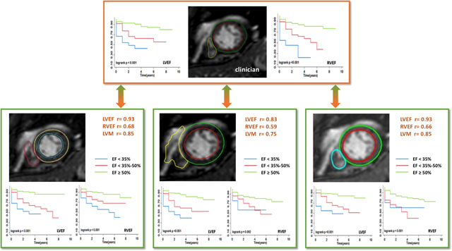
Study design and key findings. Three deep learning (DL) algorithms for determination of left and right ventricular (LV, RV) ejection fractions (EF) and LV mass were compared to reference values obtained by expert clinicians. In addition, survival analysis was performed for each of the 4 sets of measurements by dividing the patients into 3 clinically relevant EF categories for each ventricle. See text for details.

Introduction

The assessment of left and right ventricular ejection fractions (LVEF, RVEF) is fundamental for the management of patients with known or suspected heart disease (1). Left ventricular mass (LVM) is known to be associated with cardiovascular events, including incident heart failure and stroke (2). Although these measurements can be made using multiple imaging modalities, calculation of EFs remains time consuming and marred by measurement variability (3,4). Cardiac magnetic resonance (CMR) imaging is considered the reference standard for quantifying LVEF, LVM and RVEF, because the LV and RV boundaries are well defined in multiple planes, so that no geometric assumptions are required to make these measurements (5,6). Therefore, CMR has a better inter- and intra-observer reproducibility for quantifying LVEF, LVM and RVEF, compared to other imaging modalities, such as echocardiography(7). These features of CMR also make it ideal for deep learning (DL) algorithms to be applied. A significant amount of artificial intelligence (AI) research has contributed to accelerating automated CMR segmentation algorithms for calculating ventricular EF and LVM (8–11). However, it is unknown how the different AI solutions compare against each other when applied to the same database.

The key technology that underlies most modern AI solutions for the calculation of the LVEF, LVM and RVEF is DL (12,13). One type of DL architecture used is known as a convolutional neural networks, which in this case, is trained by being presented with a large number of examples in which the boundaries of the LV and RV have been annotated on the image by an expert (14,15). From this dataset, the DL algorithm autonomously learns what the features of the LV and RV boundaries are and then applies this knowledge to previously unseen datasets. The generalizability of such an algorithm is heavily reliant upon the types of examples used for training. The most robust DL algorithms have been trained not only on images obtained from patients with different disease states, but also images acquired using a variety of equipment and imaging settings (16).

In this retrospective study, we compared side-by-side fully automated EF and LVM measurements made using 3 commercial DL algorithms (DL-EF, DL-LVM) to those made by physicians interpreting CMR examinations in a clinical setting (CLIN-EF, CLIN-LVM). The specific goals of this study were: (1) to determine the agreement between DL algorithms and manual measurements made by clinical experts; (2) to determine the accuracy of DL-EF for classifying patients into clinically meaningful EF categories; (3) to determine to what extent DL-EFs and DL-LVM are associated with patient outcomes compared to CLIN-EF and CLIN-LVM.

Methods

We identified 200 consecutive patients (age 59±13years; 45%females) from a pre-existing registry of individuals undergoing vasodilator stress CMR from January 2009 to December 2015. All patients in the registry were referred for the diagnosis or evaluation of severity of ischemic heart disease. Patient demographics and clinical history were extracted from the electronic medical records. The patients were followed up for a minimum of 3 years after CMR examination by reviewing medical records and/or by telephone contacts. Clinical outcomes were a composite of all-cause death, cardiovascular death, ventricular arrhythmia admission, congestive heart failure admission, left ventricular assist device implantation and heart transplant.

Image Acquisition.

CMR imaging was performed using a 1.5-T scanner (Achieva, Philips, Best, Netherlands) with a five-element phased array cardiac coil. Retrospectively gated cine images were obtained using a steady-state free precession (SSFP) sequence, during approximately 5-second breath holds (repetition time 2.9 msec; echo time 1.5 msec; flip angle 60°; temporal resolution 30–40 msec). Standard long-axis views were obtained, including four-chamber, two-chamber, and three-chamber images. In addition, six to ten short-axis slices were obtained from the LV and RV base to the apex (slice thickness 8mm; gap 2 mm). The cine images were acquired immediately after vasodilator (regadenoson 0.4 mg) first-pass perfusion imaging using 0.5 – 0.1 mmol of gadolinium-based contrast agent was completed. The vasodilator effect was reversed with aminophylline (75 mg). After the cine images were acquired, resting perfusion and late gadolinium enhancement imaging was also performed using standard clinical pulse sequences. The protocol was approved by the Institution Review Board and informed consent was obtained from each patient.

Clinical image analysis.

The cine-CMR images were analyzed during routine clinical workflow using commercial software (Medis, Leiden, Netherlands) by the physician responsible for the CMR examination. Using the short-axis cine images, the LV and RV end-diastolic and end-systolic frames were identified. In each short-axis slice, the endocardial boundary of the LV and RV were manually delineated. LV and RV papillary muscles and trabecular tissue were included in the blood pool volume. In the LV basal slices, the LV contour was drawn to include the LV outflow tract to the level of the aortic valve cusps. The RV outflow tract was included in the RV volume to the level of the pulmonary valve. When the boundary between the atrium and ventricle was unclear, long axis views and other frames of the cardiac cycle were reviewed to facilitate the differentiation between the two chambers. Simpson’s method of disks was used to calculate LV end-diastolic mass (LVM), LV and RV end-diastolic and end-systolic volumes (EDV, ESV), and the corresponding EFs. These values were then reported and stored in the electronic medical records and eventually extracted for this study and used to divide the patient cohort into three clinically relevant groups (17): severely reduced LVEF (＜35%), mildly to moderately reduced LVEF (35–50%), and normal LVEF (≥50%).

Artificial Intelligence Image Analysis.

The DL-EF and DL-LVM were determined from cine short-axis images using three fully automated commercially available algorithms: (1) CardioAI, Arterys, San Francisco, California, USA; (2) CVI42, Circle Cardiovascular Imaging, Calgary, Alberta, Canada; and (3) SuiteHeart, Neosoft, Pewaukee, Wisconsin, USA. Since the purpose of this study was not to rank the software programs, the three vendors were anonymized by labeling them A, B, and C in no particular order. These labels are used throughout the manuscript below. Each of the vendors provided virtual training of how to optimally use their software. A single user was trained to use all three software packages and each vendor was available for feedback and input with regards to software functionality. Fully automated segmentation was then performed without any user input. Image analysis was performed using the different software packages at least two weeks apart. The automatically generated LVEDV, LVESV, LV mass, LVEF, RVEDV, RVESV, and RVEF were recorded.

Inter-Technique Comparisons.

The CLIN-EF and CLIN-LVM were considered as the reference standard, to which DL-EFs and DL-LVM generated using software A, B, and C were compared. In addition, fully automated measurements obtained using software A, B, and C were compared to each other. Finally, all datasets were also analyzed by manual segmentation using Arterys software by a member of the core lab, and the results were compared to the reference values of CLIN LVEF, LVM and RVEF, in order to assess inter-technique differences in manual measurements, related to the use of a specific vendor’s software.

Statistics.

Continuous variables were tested for normal distribution and presented as the median with interquartile range. Categorical variables were presented as absolute numbers with percentages. Values of P<0.05 were considered significant. Analyses were performed using STATA MP (version 15, college station, TX), SPSS software (version 23.0, Statistical Package for the Social Sciences, Chicago, IL) and Microsoft Excel (Microsoft, Redmond, WA).

Inter-technique comparisons included linear regression analysis with Pearson correlation coefficients and Bland-Altman analyses of biases and the corresponding confidence intervals (limits of agreement). This included the agreement between the three DL techniques (A, B and C) among themselves and against the CLIN reference, as well as between manual segmentation performed using two different software packages: one measurement performed by clinical expert using Medis and the second measurement made by core lab using Arterys. Confusion matrices were generated for each DL-EF algorithm to display the concordance/discordance with the CLIN-EF reference standard for each of the above 3 LVEF categories and thus identify the specific strengths and weaknesses of each algorithm. The sensitivity, specificity, and accuracy of each DL-EF algorithm’s ability to place the measurement into the correct category were also calculated.

Finally, intermediate term follow-up analysis was performed with reversal Kaplan-Meier methods. ROC and Kaplan-Meier analysis were performed to evaluate the diagnostic performance of CLIN-EF, CLIN-LVM and each of the DL-EF and DL-LVM to predict the future occurrence of a MACE. Pairwise log rank tests were used to test the significance of the differences between these techniques. For ROC analysis, the outcomes were treated as a binary variable, i.e. present or absent, rather than taking into account the time to each outcome in each individual patient. The ROC curves were compared against each other using C-statistic.

Reproducibility was tested by for the 3 fully automated algorithms on 20 randomly selected patients and by manual analyses by two experienced clinical experts including inter- and intra-observer reproducibility. Inter- and intra- observer variability was assessed using intraclass correlation coefficients (ICC) and coefficient of variation (CoV).

Results

Patient Demographics.

Patient characteristics are shown in Table 1 along with the relevant imaging findings. The median follow-up time for the patients was 52 months (interquartile range, 40 to 70). During pre-stress CMR exam, there were 5(3%) patients with atrial fibrillation, and 13 (7%) patients with premature ventricular contraction. In addition, 3 (1%) patients had premature ventricular contractions after intravenous regadenoson, which returned to normal sinus rhythm after intravenous aminophylline. Fifty-one (26%) of the patients experienced major adverse cardiovascular events, including: all-cause death (n=36), admission for CHF (n=21), admission for arrhythmia (need for arrhythmia treatment) (n=3), LVAD implantation (n=1), heart transplant (n=0). Figure 1 shows an example of images obtained in one patient with LV and RV boundaries detected by the three DL algorithms. DL algorithm analysis required less time per patient than the experts, and the time varied among the three algorithms: 5 seconds for algorithm A, 15 seconds for algorithm B, and 8 seconds for algorithm C.

Table 1.

Population baseline characteristics and CMR data measured in the clinical setting. Including the three subgroups according to left ventricular ejection fraction (LVEF).

Parameter	Median (interquartile range) or n (%)
Clinical	Overall (n=200)	LVEF<35% (n=27)	LVEF 35%–50% (n=61)	LVEF≥50% (n=112)
Gender, male	109 (55%)	16 (59%)	37 (61%)	56 (50%)
Age, yrs	59 ± 13	60 ± 14	62 ± 13	58 ± 13
BMI, kg/m2	29 (25–32)	28 (22–33)	29 (25–32.5)	28 (25–33)
BSA, m2	2.0 ± 0.2	1.9 ± 0.3	2.0 ± 0.2	2.0 ± 0.2
Race, %
Black	87 (44%)	17 (63%)*	30 (49%)	40 (36%)
White	89 (45%)	8 (30%)*	25 (41%)	56 (50%)
Hispanic	8 (4%)	1 (4%)	0 (0)#	7 (6%)
Asian	12 (6%)	0 (0)	2 (3%)	10 (9%)
Unknown	4 (2%)	1 (4%)	2 (3%)	1 (1%)
Medications, n (%)
Aspirin	118 (59%)	13 (48%)	40 (66%)	65 (58%)
Beta-Blocker	106 (53%)	16 (59%)	39 (64%)#	51 (46%)
ACEI/ARB	98 (49%)	19 (70%)*	34 (56%)#	45 (40%)
Statin	120 (60%)	10 (37%)*●	38 (62%)	72 (64%)
Diagnosis, n (%)
CAD	101 (51%)	11 (41%)	34 (56%)	56 (50%)
Hypertension	161 (81%)	19 (70%)	51 (84%)	91 (81%)
Cardiomyopathy	62 (31%)	25 (93%)*●	29 (48%)#	8 (7%)
Diabetes	81 (41%)	10 (37%)	28 (46%)	43 (38%)
Post-heart transplant	12 (6%)	0 (0)	3 (5%)	9 (8%)
Post-CABG	29 (15%)	3 (11%)	10 (16%)	16 (14%)
CMR
LV EDV, ml	174 (138–216)	246 (205–289)*●	204 (173–243)#	146 (123–180)
LV EDVi, ml/m2	89 (72–107)	120 (107–145)*●	102 (88–122)#	77 (62–91)
LV ESV, ml	82 (56–122)	168 (153–213)*●	115 (91–143)#	58 (3–79)
LV ESVi, ml/m2	40 (29–63)	94 (75–101)*●	58 (46–70)#	29 (23–39)
LV Mass, g	114 (92–139) n=191	132 (118–177)* n=27	129 (107–153)* n=57	105 (84–122) n=107
LV Massi, g/m2	58 (47–67) n=191	69 (60–89)* n=27	64 (53–77) n=57	52 (42–62) n=107
LV EF, %	52 (42–62)	26 (21–32)*●	43 (39–46)#	60 (55–66)
RV EDV, ml	161 (125–193)	177 (147–217)*	171 (139–194)	151 (123–184)
RV EDVi, ml/m2	81 (68–95)	91 (75–105)*	82 (68–103)	80 (65–95)
RV ESV, ml	71 (53–100)	111 (74–134)*●	77 (54–102)#	59 (49–82)
RV ESVi, ml/m2	35 (28–47)	58 (39–67)*●	38 (27–51)	32 (26–43)
RV EF, %	55 (48–61)	37 (32–45)*●	54 (48–60)#	57 (54–63)
LGE, n (%)	80 (40%)	16 (59%)*	34 (56%)#	30 (27%)
Ischemic pattern	48 (24%)	5 (19%)	23 (38%)#	20 (18%)
Non-ischemic	23 (12%)	5 (19%)	8 (13%)	10 (9%)
Both patterns	9 (5%)	6 (22%)*●	3 (5%)#	0 (0)
MACE, n (%)
All cause death	36 (18%)	10 (37%)*	16 (26%)#	10 (9%)
CV death	10 (5%)	2 (7%)	4 (7%)	4 (4%)
CHF admission	21 (11%)	6 (22%)*	9 (15%)#	6 (5%)
Arrhythmia admission	3 (1.5%)	0 (0)	2 (3%)	1 (1%)
LVAD implant	1 (0.5%)	1 (4%)	0 (0)	0 (0)
Heart transplant	0 (0)	0 (0)	0 (0)	0 (0)
Other events, n (%)
ACS	37 (19%)	6 (22%)	14 (23%)	17 (15%)
CABG	12 (6%)	1 (4%)	7 (11%)#	4 (4%)

^*P<0.05, LVEF < 35% and LVEF ≥50%

^#P<0.05, LVEF 35%−50% and LVEF ≥50%

^●P<0.05, LVEF < 35% and LVEF 35%−50%

Abbreviations: BMI – body mass index, ACEI –converting enzyme inhibitor, ARB – angiotensin receptor blocker, CAD – coronary artery disease, CABG – coronary artery bypass graft, LV – left ventricular, RV – right ventricular, EDV – end-diastolic volume, ESV - end-systolic volume, EF – ejection fraction, LGE – late gadolinium enhancement, MACE – major adverse cardiovascular event, CV – cardiovascular, ACS – acute coronary syndrome, CHF – congestive heart failure, LVAD – left ventricular assist device.

Figure 1. Example of images of one patient with contours detected by three DL algorithms.

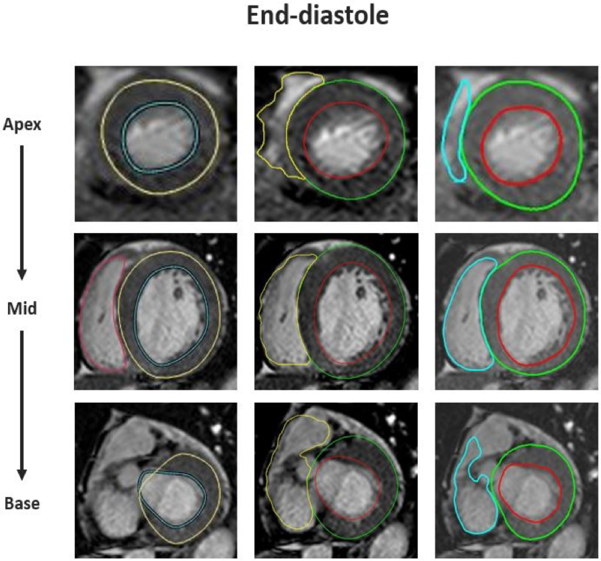
Endocardial and epicardial contours of LV and endocardial contours of RV from apex (top) to base (bottom) detected automatically by three software packages (shown from left to right in no particular order). Note poorly defined RV boundaries in the apical slice and last basal slice identified by all three algorithms. But the LV and RV boundaries automatically detected in the mid-slice are accurate. This patient was diagnosed with ischemic cardiomyopathy with CLIN-LVEF 42% and CLIN-RVEF 48%.

Relationship between CLIN-EF and DL-EF.

The correlations between CLIN-EF and DL-EF ranged between 0.83～0.93 for the LV and 0.59～0.68 for the RV (Figure 2). The results of Bland-Altman analyses for the 3 DL algorithms for both ventricles are depicted in Figure 3, which shows the biases with the corresponding limits of agreement. Algorithm A underestimated LVEF, while Algorithm B slightly overestimated it, and Algorithm C had no systematic error, as reflected by biases of 1% for A, −4% for B, 0% for C. For RVEF, the biases were: 8% for A, 1% for B, −4% for C, reflecting worse performance than for the left ventricle for all three algorithms, as evidenced by larger biases and wider limits of agreement. Figure 4 shows the distribution of the absolute differences between CLIN-EF and each of the DL-EF algorithms. Compared to the CLIN-EF, most DL-EF errors for the LV were small: 36–47% of measurement within 3% difference and 53–78% within 5% difference, depending on the algorithm. For algorithm A, 71 (36%) cases were within 3% and 140 (70%) cases were within 5% of CLIN-LVEF. For algorithm B, 57 (29%) cases were within 3% and 105 (53%) cases were within 5% of CLIN-LVEF. For algorithm C, 94 (47%) cases were within 3% and 156 (78%) cases were within 5% of CLIN-LVEF.

Figure 2. Linear regression plots comparing CLIN and the three commercial DL algorithms (A, B, and C):

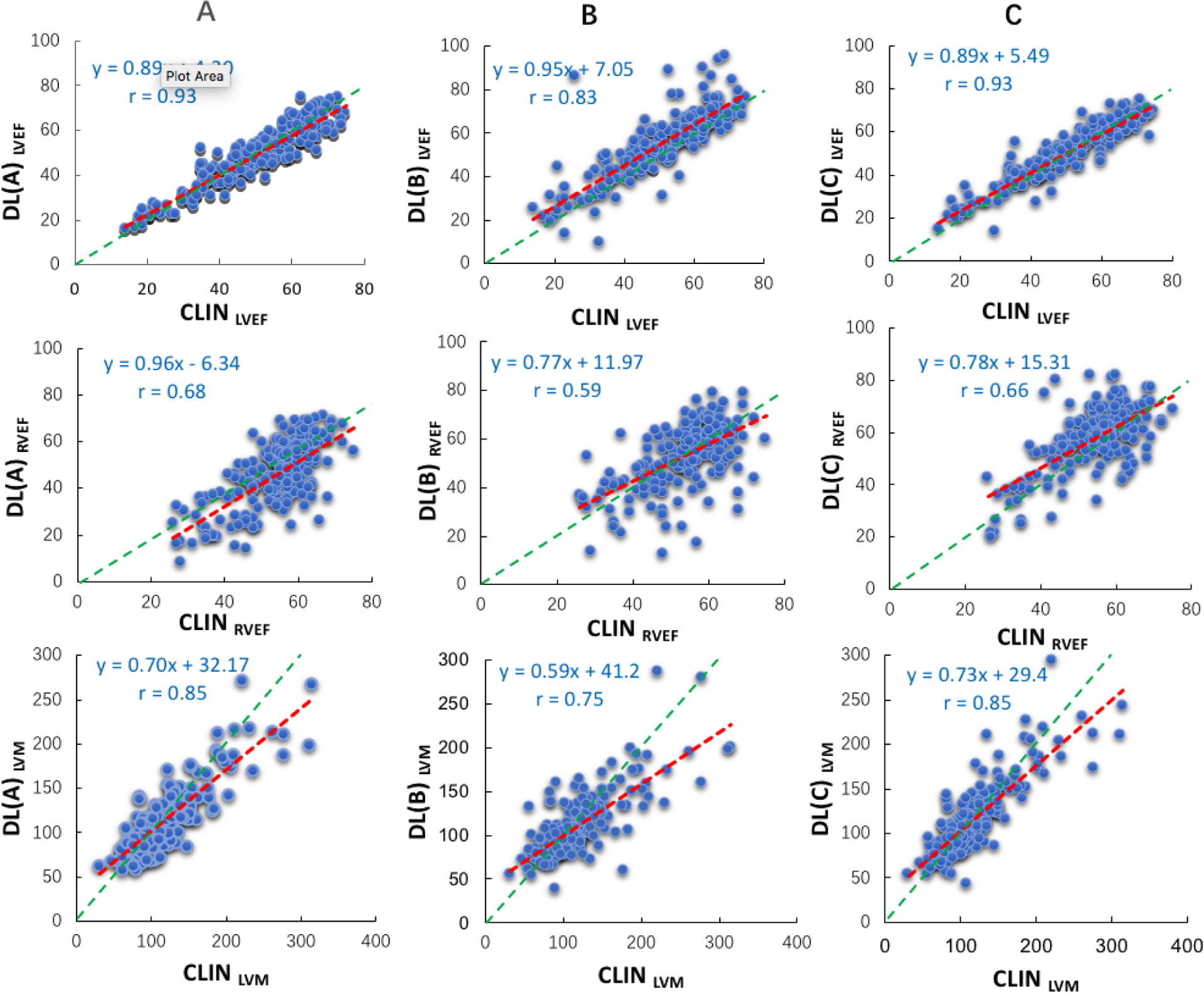
LVEF (top), RVEF (mid), and LVM (bottom). Red lines represent the regression lines, while the green lines represent perfect agreement (unity lines).

Figure 3. Bland-Altman plots comparing CLIN and the three commercial DL algorithms (A, B, and C):

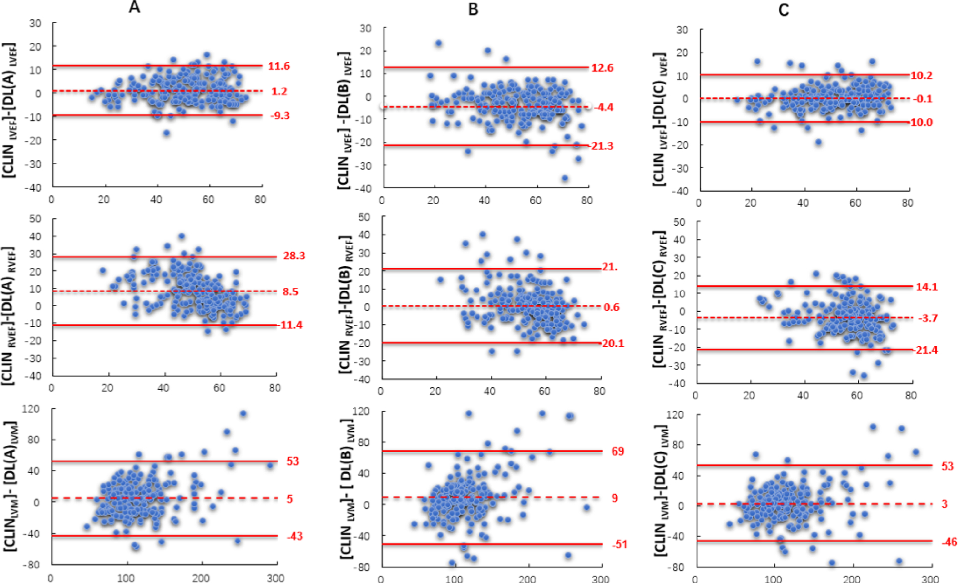
LVEF (top), RVEF (mid), and LVM (bottom). Biases are shown with the corresponding confidence intervals (limits of agreement).

Figure 4. Histograms showing the distribution of absolute differences between CLIN-EF and the three commercially available DL-EF algorithms.

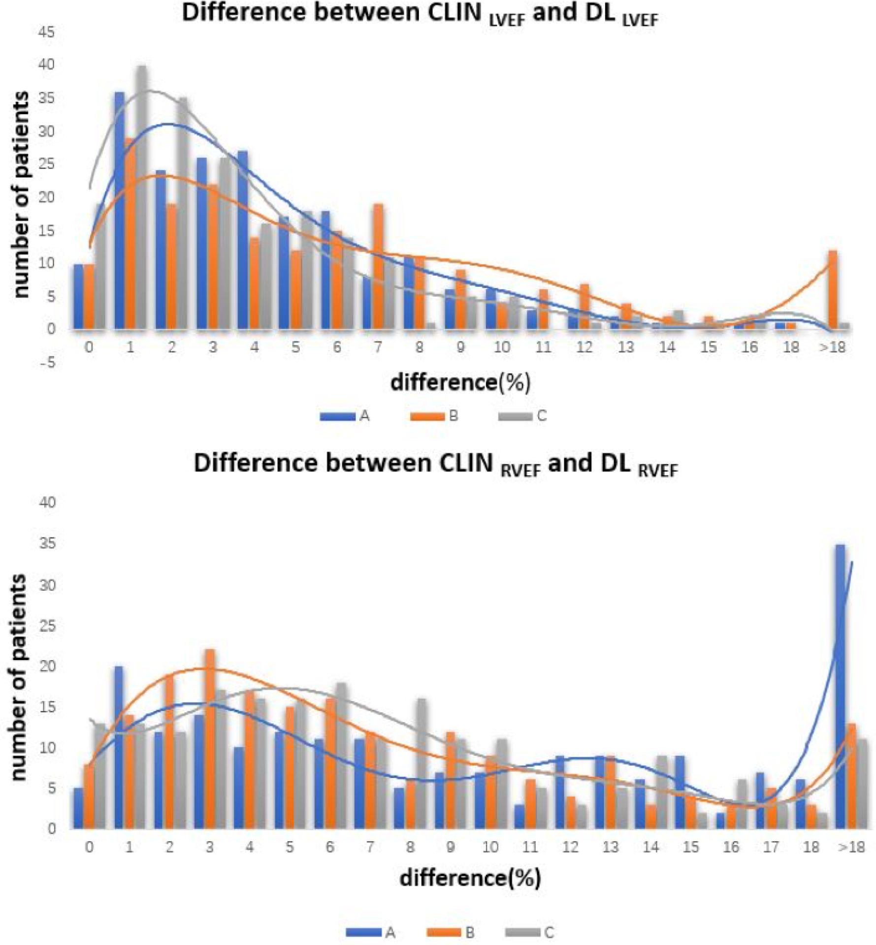
A, B, and C for the left ventricle (top) and the right ventricle (bottom).

In contrast, for the RV, the percentages of smaller errors were considerably lower: 19–21% of measurement were within 3% and 37–48% were within 5%, depending on the algorithm. For algorithm A, 37 (19%) cases were within 3% and 73 (37%) cases were within 5% of CLIN-RVEF. For algorithm B, 41 (21%) cases were within 3% and 96 (48%) cases were within 5% of CLIN-RVEF. For algorithm C, 39 (20%) cases were within 3% and 87 (44%) cases were within 5% of CLIN-RVEF.

Of note, differences of >10% were noted in 5–18% of cases for the LV, and in a considerably larger number of cases, 23–43% for the RV. For the LV, 11 (6%) cases for algorithm A, 35 (18%) cases for algorithm B, 10 (5%) cases for algorithm C showed differences >10% from CLIN-LVEF. For the RV, 86 (43%) cases for algorithm A, 50 (25%) cases for algorithm B, 46 (23%) cases for algorithm C were >10% off relative to CLIN-LVEF.

Relationship between CLIN-LVM and DL-LVM.

DL-LVM measurements were less accurate than LVEF when compared to CLIN- LVM (Figures 2 and 3). For LV mass, the correlations between CLIN- LVM and DL-LVM ranged between 0.75～0.85. Bland-Altman analyses of comparison between CLIN-LVM and DL-LVM resulted in biases of 5 g for algorithm A, 9 g for B, and 3 g for C.

Comparisons between DL techniques.

For all three parameters, including LVEF, RVEF and LVM, the levels of agreement were similar to those between the DL techniques and the clinical reference (Table 2).

Table 2.

Inter-technique comparisons between the three DL algorithms (A, B and C), including Pearson’s correlation coefficients and Bland-Altman biases.

Parameter	Inter-DL algorithm	r	Bias (±SD)
LVEF	A - B	0.83	−6 (±9)
	A - C	0.93	−1 (±5)
	B - C	0.83	4 (±9)
LVM	A - B	0.85	4 (±20)
	A - C	0.91	−2 (±17)
	B - C	0.85	−6 (±21)
RVEF	A - B	0.48	−8 (±14)
	A - C	0.60	−12 (±12)
	B - C	0.45	−4 (±13)

Agreement between manual techniques.

Manual measurements using the Medis and Arterys software packages resulted in excellent correlations as reflected by r-values of 0.95 for the LVEF, 0.89 for RVEF and 0.91 for LVM and small biases with narrow limits of agreement (Table 3). This analysis additionally served as a comparison between the clinical readers and a core lab measurement.

Table 3.

Inter-technique comparisons between the two manual techniques (clinical expert versus core lab interpretation), including Pearson’s correlation coefficients and Bland-Altman biases.

Parameter	r	Bias (±SD)
LVEF	0.95	−1 (±5)
LVM	0.91	−1 (±5)
RVEF	0.89	−8 (±14)

Classification into Ejection Fraction Categories.

Based on CLIN-EF, 27 subjects had severely reduced LVEF, 61 had moderately reduced LVEF, and 112 had preserved LVEF. The three DL-LVEF algorithms resulted in accurate classification in 80 – 86% of the patients, while the lowest rates of accurate classifications were noted in the mid LVEF category of 35–50% (Figure 5).

Figure 5. Confusion matrices showing accuracy of DL-LVEF to correctly categorize into clinically meaningful EF groups as defined by the clinically reported LVEF (CLIN-LVEF).

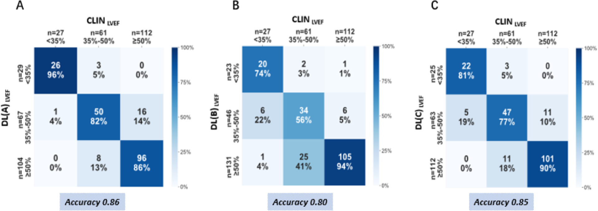
Across true label rows, the numbers in the boxes represent the percentage of labels classified for each group. Color intensity corresponds to percentage, see heat map on the right.

Comparison of CLIN-EF and DL-EF for risk prediction.

As expected, both LVEF and RVEF were associated with MACE in our cohort. Based on ROC analysis, the LV and RV CLIN-EF had C-statistic value of 0.74 and 0.68, respectively, for predicting MACE during the follow-up period. The 3 DL-EF algorithms had C-statistic values for the LV, algorithm A 0.73 (95% CI, 0.65–0.81), algorithm B 0.73 (95% CI, 0.66–0.82), algorithm C 0.72 (95% CI, 0.65–0.81). For the RV, algorithm A 0.68 (95% CI, 0.60–0.77), algorithm B 0.64 (95% CI, 0.55–0.73), algorithm C 0.63 (95% CI, 0.54–0.72). Importantly, there was no significant difference between the ability of CLIN-EF and DL-EF algorithms to predict outcomes (Figure 6). For LVM, there was moderate ability to predict MACE, and no significant difference between CLIN-LVM and DL-LVM (Figure 6).

Figure 6. ROC analysis comparing the CLIN-EF, CLIN-LVM and the three DL-EF, DL-LVM algorithms for predicting MACE for the left ventricle (left), the right ventricle (mid) and left ventricular mass (right).

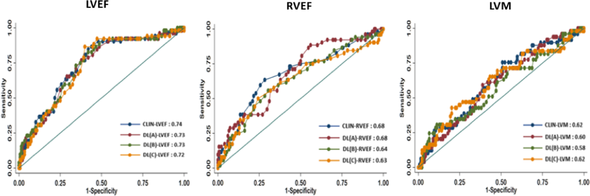
There was no statistical difference between any of the curves for either parameters.

Kaplan-Meier survival curves illustrated significant difference between three EF cutoff subgroups for both CLIN-EFs and DL-EFs, which were more clear-cut for the left ventricle (Figure 7), compared to the right ventricle (Figure 8). While generally, patients with higher EFs had better chances of survival, the ability to differentiate outcomes between moderately and severely reduced RVEF was limited for the three DL algorithms.

Figure 7. Kaplan-Meier estimates of survival for patients with LVEF<35%, 35–50%, ≥50%.

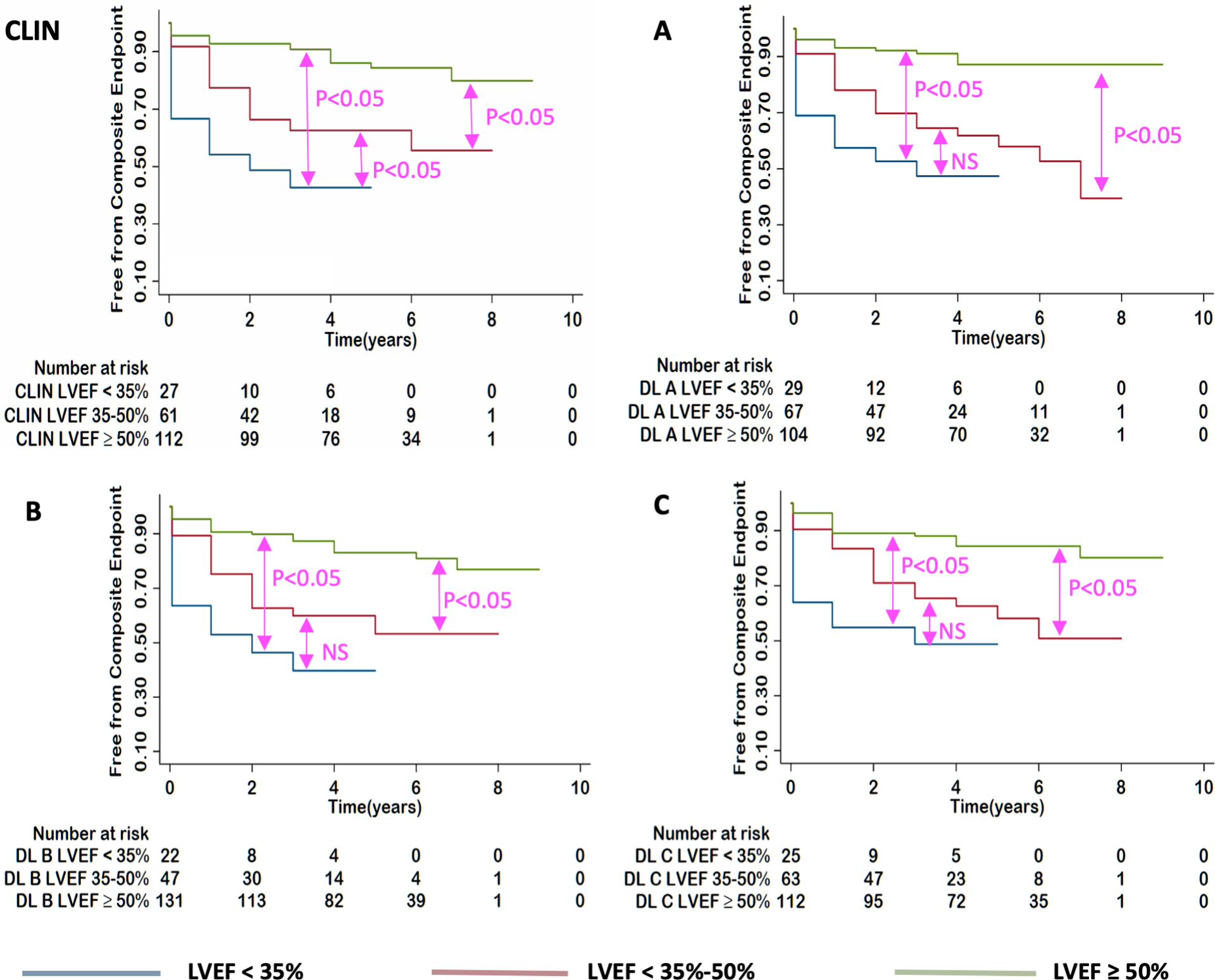
for: CLIN-EF, DL(A)-EF, DL(B)-EF and DL(C)-EF. P-values show the results of pairwise log rank tests.

Figure 8. Kaplan-Meier estimates of survival for patients with RVEF<35%, 35–50%, ≥50%.

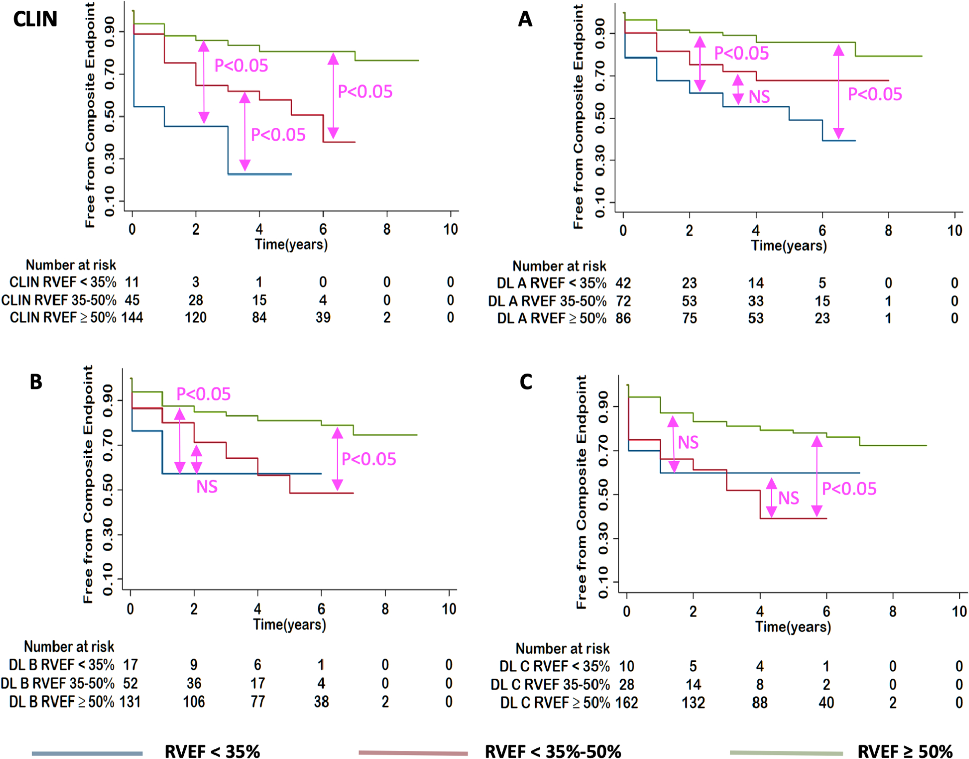
for: CLIN-EF, DL(A)-EF, DL(B)-EF and DL(C)-EF from left to right. P-values show the results of pairwise log rank tests.

Reproducibility.

The intraclass correlations for the inter- and intra-observer variability of manual measurements made by the clinical experts were 0.90 and 0.93 for the LVEF, 0.88 and 0.94 for the LVM, 0.55 and 0.81 RVEF, respectively. In contrast, DL algorithms showed zero variability in all repeated measurements, due to their fully-automated, deterministic nature.

Discussion

In this study, we sought to determine the relationship between the clinical impact of physician reported LVEF, LVM and RVEF and those determined automatically by three commercial DL algorithms. The DL-LVEFs and DL-LVMs showed good agreement with CLIN-LVEF and CLIN-LVM, as evidenced by the strong correlations and small biases, albeit with considerable inter-technique differences in individual patients, reflected by the moderate limit of agreement. We also found that the DL-LVEF algorithms accurately classified LVEF into clinically meaningful categories, which accurately predict clinical outcomes with no significant differences between CLIN-EF and DL-EF algorithms. Importantly, the three subgroups of CLIN-LVEF and DL-LVEF were significant predictors of the MACE. In contrast, the association between DL-RVEF and outcomes was not as clear from the Kaplan-Meier curves. (See Central Illustration).

Left and right ventricular EF are key imaging biomarkers, which are used routinely for clinical decision making. Absolute EF cutoff values are often used to determine when to initiate pharmacotherapy, device therapy or surgical intervention (18–21). CMR is a versatile cardiovascular imaging modality and is considered the reference standard for the quantification of cardiac size and function (22). Image segmentation is an important initial step for most forms of cardiac chamber quantification (10,23). It partitions the image into a number of anatomically meaningful regions, such as the various chambers, the epicardial and endocardial boundaries, from which quantitative measures can be obtained (24). Although it is the current reference standard, manual quantification of chamber size and function from cine CMR images remains somewhat subjective and time-consuming (25,26). The recent introduction of artificial intelligence, particularly DL methods using convolutional neural networks, hold the promise of fully automating quantification (8,9,27,28).

Several studies have compared automated segmentation with manually acquired data and found that the accuracy of automated measures is comparable to human expert performance (4,29–33). While promising, these studies had several limitations, including training the algorithms on homogenous CMR sequences limiting widespread applicability, small sample sizes, semi-automated segmentation requiring manual correction, and focus on a single algorithm. To circumvent these limitations, we tested three different commercial DL algorithms on stress CMR images. We selected stress CMR not only because it is a common indication for CMR imaging, but also because we suspected that the algorithms may not perform as well in this situation since the images used to quantify EF and LVM are acquired after the administration of a gadolinium-based contrast agent (34). The training datasets used to create the algorithms are unlikely to have included this type of images. Nevertheless, we found that the agreement between CLIN and DL measurements determined from stress CMR images was good for each of the algorithms used to calculate LVEF and LVM, but only modest for RVEF. Our correlation coefficients were lower than reported in prior studies (8,29,33), likely because of the effects of contrast on the image quality. In our study, the DL-EF for the left ventricle was within 5% of the CLIN-EF for the majority of patients using all 3 algorithms. However, for the right ventricle, two of the DL-EF algorithms had an error >5% for the majority of patients. This is likely due to the unique morphology, thinner myocardium, and higher trabeculation burden of the RV, which pose a challenge for detecting boundaries for both the clinical expert and the automated DL algorithms (23,35) (Figure 1). Basal short-axis slice was most often inaccurately identified by the DL algorithms, particularly for the RV in connection with pulmonary artery and right atrium. Furthermore, occasionally, the RV apex was not identified by the DL algorithms in apical slices in cases of pathological RV morphology.

In addition, we studied the accuracy of DL-EF for classifying patients into clinically meaningful EF categories: LVEF＜35% (often considered a cutoff of defibrillator implantation), LVEF 35–50% (the range when the initiation of medical therapy is considered), and preserved (≥50%) (36). We found that the DL-LVEF overall performed well for classification of LVEFs ＜35% and ≥50%. Notably, clinicians are particularly skilled at determining accurate LVEF when the systolic function is close to 35%, likely due to being biased by clinical factors when close to clinically important cut-offs. In contrast, we found poor agreement between DL-LVEF and CLIN-LVEF for classification of LVEF 35–50%. Presumably, there may be geometrical and structural abnormalities, such as segmental dyskinesia or heterogeneous wall thickness, making it difficult to clearly identify the LV endocardial boundary by DL algorithms.

Nevertheless, despite the difference between the calculated CLIN and DL EF and LVM, there was no significant difference between the ability of CLIN and DL algorithms to predict major adverse cardiovascular outcomes in our study. These results add to the current literature establishing CMR AI models for predicting clinical adverse events (37,38), and suggest that DL models for EF may lead to a more automated evaluation of prognosis.

Although our data show that the DL-algorithms are fast, fully automated, thus eliminating the need for human input, have perfect reproducibility due to their deterministic nature and perform fairly well when compared to a clinical expert, there is room for improvement. In fact, the developers of the three DL algorithms continuously refine and optimize the performance of these products by increasing the diversity of the training datasets. The accuracy of a DL-algorithm is clearly related to the breadth of image types and disease states that it has been exposed to in the training phase. Our study was comprised entirely of contrast-enhanced cine images and the endocardial boundaries were likely to be less well defined than in images acquired without contrast enhancement. It is possible that the automated DL approach will perform better if future training datasets also include contrast-enhanced images. Currently, most commercial DL algorithms are trained by being exposed to individual still frames of cine videos acquired in the short axis plane. However, when a clinical expert interprets a study, they also consider patterns of the cardiac motion and orthogonal views to differentiate between structures such as the atrium and ventricle. Next generation of DL algorithms, which utilize the long-axis views in addition to the short-axis views to better delineate boundaries are already being developed and will likely further improve the ability to quantify cardiac chamber size and function. Future innovations for cardiac segmentation should also take into account cardiac motion.

Limitations:

This was a single-center study performed in a relatively small sample of unselected patients referred for vasodilator stress CMR. Therefore, the possibility of different results if applied to a different cohort in a different setting cannot be ruled out. In addition, the focus of our analysis was to compare the performance between multiple DL algorithms and standard clinical methodology; thus, the impact of artifacts and other factors influencing image quality was not considered. Also, while on a group level, the automated segmentation algorithms performed with similar accuracy to clinical analysis in predicting MACE, there were important mis-classifications on a patient level. To improve the performance of the automated algorithms, it may be helpful to incorporate local training sets as part of the development pipeline in the future. This was not part of the current study. Finally, in our ROC analysis, the outcomes were treated as a binary variable, i.e. present or absent, rather than taking into account the time to each outcome in each individual patient, which would be more rigorous.

Conclusions:

The fully automated DL algorithms correlated highly with the clinical expert’s LVEF measurements, but not RVEF. Nevertheless, up to 20% of cases were classified into the incorrect LVEF category by the DL algorithms. For RVEF, the algorithms had a >5% error in the majority of patients. Further development of the DL algorithms is needed before supervision by a clinical expert could be considered unnecessary. Despite these limitations, DL-derived EFs predicted adverse cardiovascular events as well as an expert.

Clinical Perspectives:

COMPETENCY IN MEDICAL KNOWLEDGE:

Deep learning segmentation algorithms are highly efficient and provide accurate information, when compared to the conventional methodology.

COMPETENCY IN PATIENT CARE AND PROCEDUARAL SKILLS:

Fully automated EF and LVM have similar predictive value to that of the conventional methodology.

TRANSLATIONAL OUTLOOK:

This is the first study to compare three commercial, fully automated DL techniques in the context of stress CMR.

ABBREVIATIONS:

CLIN

clinical expert

DL

deep learning

CMR

cardiac magnetic resonance

LVEF

left ventricular ejection fraction

RVEF

Right ventricular ejection fraction

LVM

left ventricular mass

REFERENCES

- 1.Marwick TH. Ejection Fraction Pros and Cons: JACC State-of-the-Art Review. Journal of the American College of Cardiology 2018;72:2360–2379. [DOI] [PubMed] [Google Scholar]
- 2.Abdi-Ali A, Miller RJH, Southern D et al. LV Mass Independently Predicts Mortality and Need for Future Revascularization in Patients Undergoing Diagnostic Coronary Angiography. JACC Cardiovascular imaging 2018;11:423–433. [DOI] [PubMed] [Google Scholar]
- 3.Bellenger NG, Burgess MI, Ray SG et al. Comparison of left ventricular ejection fraction and volumes in heart failure by echocardiography, radionuclide ventriculography and cardiovascular magnetic resonance. Are they interchangeable? European Heart Journal 2000;21:1387–1396. [DOI] [PubMed] [Google Scholar]
- 4.Wood PW, Choy JB, Nanda NC, Becher H. Left ventricular ejection fraction and volumes: It depends on the imaging method. Echocardiography 2014;31:87–100. [DOI] [PMC free article] [PubMed] [Google Scholar]
- 5.Petersen SE, Aung N, Sanghvi MM et al. Reference ranges for cardiac structure and function using cardiovascular magnetic resonance (CMR) in Caucasians from the UK Biobank population cohort. Journal of Cardiovascular Magnetic Resonance 2017;19:1–19. [DOI] [PMC free article] [PubMed] [Google Scholar]
- 6.Foley TA, Mankad SV, Anavekar NS et al. Measuring left ventricular ejection fraction-techniques and potential pitfalls. European Cardiology 2012;8:108–114. [Google Scholar]
- 7.Hoffmann R, Barletta G, Von Bardeleben S et al. Analysis of left ventricular volumes and function: A multicenter comparison of cardiac magnetic resonance imaging, cine ventriculography, and unenhanced and contrast-enhanced two-dimensional and threedimensional echocardiography. Journal of the American Society of Echocardiography 2014;27:292–301. [DOI] [PubMed] [Google Scholar]
- 8.Backhaus SJ, Staab W, Steinmetz M et al. Fully automated quantification of biventricular volumes and function in cardiovascular magnetic resonance: Applicability to clinical routine settings. Journal of Cardiovascular Magnetic Resonance 2019;21:1–13. [DOI] [PMC free article] [PubMed] [Google Scholar]
- 9.Bai W, Sinclair M, Tarroni G et al. Automated cardiovascular magnetic resonance image analysis with fully convolutional networks. Journal of Cardiovascular Magnetic Resonance 2018;20:1–12. [DOI] [PMC free article] [PubMed] [Google Scholar]
- 10.Peng P, Lekadir K, Gooya A, Shao L, Petersen SE, Frangi AF. A review of heart chamber segmentation for structural and functional analysis using cardiac magnetic resonance imaging. Magnetic Resonance Materials in Physics, Biology and Medicine 2016;29:155–195. [DOI] [PMC free article] [PubMed] [Google Scholar]
- 11.Suinesiaputra A, Sanghvi MM, Aung N et al. Fully-automated left ventricular mass and volume MRI analysis in the UK Biobank population cohort: evaluation of initial results. International Journal of Cardiovascular Imaging 2018;34:281–291. [DOI] [PMC free article] [PubMed] [Google Scholar]
- 12.Chen C, Qin C, Qiu H et al. Deep Learning for Cardiac Image Segmentation: A Review. Frontiers in Cardiovascular Medicine 2020;7. [DOI] [PMC free article] [PubMed] [Google Scholar]
- 13.Xu B, Kocyigit D, Grimm R, Griffin BP, Cheng F. Applications of artificial intelligence in multimodality cardiovascular imaging: A state-of-the-art review. Progress in Cardiovascular Diseases 2020. [DOI] [PubMed] [Google Scholar]
- 14.Leiner T, Rueckert D, Suinesiaputra A et al. Machine learning in cardiovascular magnetic resonance: Basic concepts and applications. Journal of Cardiovascular Magnetic Resonance 2019;21:1–14. [DOI] [PMC free article] [PubMed] [Google Scholar]
- 15.Tao Q, Lelieveldt BPF, Van Der Geest RJ. Deep learning for quantitative cardiac MRI. American Journal of Roentgenology 2020;214:529–535. [DOI] [PubMed] [Google Scholar]
- 16.Siegersma KR, Leiner T, Chew DP, Appelman Y, Hofstra L, Verjans JW. Artificial intelligence in cardiovascular imaging: state of the art and implications for the imaging cardiologist. Netherlands Heart Journal 2019;27:403–413. [DOI] [PMC free article] [PubMed] [Google Scholar]
- 17.McMurray JJV, Adamopoulos S, Anker SD et al. ESC Guidelines for the diagnosis and treatment of acute and chronic heart failure 2012: The Task Force for the Diagnosis and Treatment of Acute and Chronic Heart Failure 2012 of the European Society of Cardiology. Developed in collaboration with the Heart. European heart journal 2012;33:1787–1847. [DOI] [PubMed] [Google Scholar]
- 18.Al-Khatib SM, Stevenson WG, Ackerman MJ et al. 2017 AHA/ACC/HRS Guideline for Management of Patients With Ventricular Arrhythmias and the Prevention of Sudden Cardiac Death, 2018.
- 19.Dahl JS, Eleid MF, Michelena HI et al. Effect of left ventricular ejection fraction on postoperative outcome in patients with severe aortic stenosis undergoing aortic valve replacement. Circulation: Cardiovascular Imaging 2015;8:1–8. [DOI] [PubMed] [Google Scholar]
- 20.Nishimura RA, Otto CM, Bonow RO et al. 2014 AHA/ACC guideline for the management of patients with valvular heart disease: A report of the American college of cardiology/American heart association task force on practice guidelines. Journal of the American College of Cardiology 2014;63. [DOI] [PubMed] [Google Scholar]
- 21.Yancy CW, Jessup M, Bozkurt B et al. 2016 ACC/AHA/HFSA Focused Update on New Pharmacological Therapy for Heart Failure: An Update of the 2013 ACCF/AHA Guideline for the Management of Heart Failure: A Report of the American College of Cardiology/American Heart Association Task Force on Clinic. Journal of Cardiac Failure 2016;22:659–669. [DOI] [PubMed] [Google Scholar]
- 22.Pennell DJ, Sechtem UP, Higgins CB et al. Clinical indications for cardiovascular magnetic resonance (CMR): Consensus Panel report. European Heart Journal 2004;25:1940–1965. [DOI] [PubMed] [Google Scholar]
- 23.Petitjean C, Dacher JN. A review of segmentation methods in short axis cardiac MR images. Medical Image Analysis 2011;15:169–184. [DOI] [PubMed] [Google Scholar]
- 24.Schulz-Menger J, Bluemke DA, Bremerich J et al. Standardized image interpretation and postprocessing in cardiovascular magnetic resonance - 2020 update : Society for Cardiovascular Magnetic Resonance (SCMR): Board of Trustees Task Force on Standardized Post-Processing. Journal of cardiovascular magnetic resonance : official journal of the Society for Cardiovascular Magnetic Resonance 2020;22:19–19. [DOI] [PMC free article] [PubMed] [Google Scholar]
- 25.Miller CA, Jordan P, Borg A et al. Quantification of left ventricular indices from SSFP cine imaging: Impact of real-world variability in analysis methodology and utility of geometric modeling. Journal of Magnetic Resonance Imaging 2013;37:1213–1222. [DOI] [PubMed] [Google Scholar]
- 26.Suinesiaputra A, Bluemke DA, Cowan BR et al. Quantification of LV function and mass by cardiovascular magnetic resonance: Multi-center variability and consensus contours. Journal of Cardiovascular Magnetic Resonance 2015;17:1–8. [DOI] [PMC free article] [PubMed] [Google Scholar]
- 27.Bernard O, Lalande A, Zotti C et al. Deep Learning Techniques for Automatic MRI Cardiac Multi-Structures Segmentation and Diagnosis: Is the Problem Solved? IEEE Transactions on Medical Imaging 2018;37:2514–2525. [DOI] [PubMed] [Google Scholar]
- 28.Tan LK, McLaughlin RA, Lim E, Abdul Aziz YF, Liew YM. Fully automated segmentation of the left ventricle in cine cardiac MRI using neural network regression. Journal of Magnetic Resonance Imaging 2018;48:140–152. [DOI] [PubMed] [Google Scholar]
- 29.Bhuva AN, Bai W, Lau C et al. A Multicenter, Scan-Rescan, Human and Machine Learning CMR Study to Test Generalizability and Precision in Imaging Biomarker Analysis. Circulation: Cardiovascular Imaging 2019;12:1–11. [DOI] [PubMed] [Google Scholar]
- 30.Luo G, Dong S, Wang W et al. Commensal correlation network between segmentation and direct area estimation for bi-ventricle quantification. Medical Image Analysis 2020;59:101591–101591. [DOI] [PubMed] [Google Scholar]
- 31.Marino M, Corsi C, Maffessanti F, Patel AR, Mor-Avi V. Objective selection of short-axis slices for automated quantification of left ventricular size and function by cardiovascular magnetic resonance. Clinical Imaging 2016;40:617–623. [DOI] [PubMed] [Google Scholar]
- 32.Purmehdi H, Hareendranathan AR, Noga M, Punithakumar K. Right Ventricular Segmentation from MRI Using Deep Convolutional Neural Networks. Proceedings of the Annual International Conference of the IEEE Engineering in Medicine and Biology Society, EMBS; 2019:4020–4023. [DOI] [PubMed] [Google Scholar]
- 33.Zange L, Muehlberg F, Blaszczyk E et al. Quantification in cardiovascular magnetic resonance: Agreement of software from three different vendors on assessment of left ventricular function, 2D flow and parametric mapping. Journal of Cardiovascular Magnetic Resonance 2019;21:1–14. [DOI] [PMC free article] [PubMed] [Google Scholar]
- 34.Fathi A, Weir-Mccall JR, Struthers AD, Lipworth BJ, Houston G. Effects of contrast administration on cardiac MRI volumetric, flow and pulse wave velocity quantification using manual and software-based analysis. British Journal of Radiology 2018;91. [DOI] [PMC free article] [PubMed] [Google Scholar]
- 35.Avendi MR, Kheradvar A, Jafarkhani H. Automatic segmentation of the right ventricle from cardiac MRI using a learning-based approach. Magnetic Resonance in Medicine 2017;78:24392448. [DOI] [PubMed] [Google Scholar]
- 36.Yancy CW, Jessup M, Bozkurt B et al. 2013 ACCF/AHA guideline for the management of heart failure: A report of the american college of cardiology foundation/american heart association task force on practice guidelines. Circulation 2013;128:240–327. [DOI] [PubMed] [Google Scholar]
- 37.Dawes TJW, De Marvao A, Shi W et al. Machine learning of threedimensional right ventricular motion enables outcome prediction in pulmonary hypertension: A cardiac MR imaging study. Radiology 2017;283:381–390. [DOI] [PMC free article] [PubMed] [Google Scholar]
- 38.Samad MD, Wehner GJ, Arbabshirani MR et al. Predicting deterioration of ventricular function in patients with repaired tetralogy of Fallot using machine learning. European Heart Journal Cardiovascular Imaging 2018;19:730–738. [DOI] [PMC free article] [PubMed] [Google Scholar]