Real Time Reduced Order Model for Angiography Fractional Flow Reserve

Abstract

Background and Objectives:

Fractional flow reserve (FFR) is the gold standard for quantification of coronary stenosis and pressure wire is the gold standard for measuring FFR. Recently, computational fluid dynamics (CFD) methods have been used to compute FFR less invasively using images obtained from coronary angiography. This approach is, however, computationally intensive and solutions to reduce computation time are clearly required.

Methods:

We hypothesized that FFR can be calculated instantly using a reduced order model (ROM) derived using response surface method (RSM) for simulation modeling in lieu of the computationally intensive CFD. Specifically, eleven physiological and anatomical factors known to affect FFR were selected as input variables, and Plackett–Burman analysis was performed in conjunction with CFD on model arteries to identify set of variables affecting FFR the most. Based on the Box–Behnken design, a mathematical model was developed to compute FFR using the retained set of variables.

Results:

The model fidelity was tested on a cohort of 90 patients (100 coronary arteries) with known pressure-wire FFR. FFR derived from this ROM had a strong correlation with pressure-wire FFR with sensitivity of 89.4%, specificity of 100% and area under curve of 0.947 (p < 0.05).

Conclusions:

The ROM method can be used to reliably calculate FFR in patients with coronary stenosis and able to replace time-consuming CFD-based FFR estimation and provide instead a real-time calculation method.

Introduction

Fractional flow reserve (FFR) is the gold standard for quantifying the degree of coronary artery stenosis [1]. FFR is the ratio of maximal blood flow distal to a stenotic lesion to maximal flow in the same artery if hypothetically normal. It is an index that reveals the ischemic potential of individual lesions [2]. Normal FFR is 1 and FFR ≤ 0.80 is considered hemodynamically significant and used as indicator of stenosis [1]. FFR is typically measured in cardiac catheterization laboratory using pressure-wire [3]. This requires the insertion of pressure-sensor guidewire in the coronary and Adenosine injection for inducing hyperemia[4]. These requirements contribute to the low adoption rate of FFR in clinical practice since they invoke a combination of factors related to practicality, time, and cost [5].

Coronary angiography to assess degree of stenosis does not reveal the physiological impact on the coronary circulation. Thus, identifying the accurate hemodynamic significance of the stenosis can fail frequently if evaluated solely based on angiography, especially in the range of intermediate stenosis of 40 to 80% [6]. Recently, advanced computational fluid dynamics (CFD) techniques have been applied to human coronary CT angiography (CCTA) imaging datasets providing a more comprehensive approach that adds to the diagnostic value of CCTA [7]. These were shown to enhance the diagnostic performance of CCTA for detecting hemodynamically significant coronary artery disease [5, 8]. FFR can also be computed using CFD from the coronary angiogram and it is an available method for assessing blood circulation through coronary artery [9-11]. CFD-based FFR does not require insertion of a pressure-sensitive wire and hyperemia induction [12]. CFD-based FFR computation, however, is currently not real-time with “push of a button”. Indeed, calculation of CFD-based FFR requires 3D rendering of the coronary segment of interest, mesh generation and flow simulation. Practically, for any solution to be viable for real-time use in cardiac catheterization lab, one has to provide FFR results in, ideally, less than 1 minute. To address this problem, we propose a novel ROM to compute FFR from angiograms by RSM in real time. RSM is commonly used to optimize experimental methods or processes or find important interactions between factors in a complex system. ROMs are considered as computationally inexpensive mathematical representations that can analyze near real-time[13, 14]. The major advantage of this approach over the competing solutions, including CFD based ones, is its potential to deliver real-time results within seconds. Given the favorable attributes of this technology, such as minimal computational power requirement and ease of use, we fully anticipate that our model can run on an off-the-shelf workstation. Therefore, equipment cost for adopting institutions would be minimal as the software could easily run on existing computers in cardiac catheterization lab. In this study, significant factors affecting FFR were selected using Plackett–Burman method in conjunction with CFD since CFD allowed analysis of different combinations of input variables in a way that would have been impractical to do experimentally. A Box-Behnken design was deployed to establish a ROM that governs the relationship between the significant factors identified from RSM and FFR. We then tested the model in 100 coronary arteries from 90 patients with known pressure-wire FFR for clinical validation.

Methods

Patient Population and 3D Rendering

In this study, Patients with left anterior descending artery [LAD], left circumflex [LCx]/obtuse marginal [OM] and right coronary artery [RCA] were included. Exclusion criteria were: Coronary arteries with bifurcational lesions (i.e., only straight segment lesions), and coronary arteries distally protected by bypass grafts. Table 1 shows Patients’ characteristics. One hundred arteries from ninety patients who had undergone FFR measurements. Previously, Three-dimensional (3D) reconstruction of coronary arteries was performed with the CAAS 7.5 QCA-3D system. The study protocol was approved by the institutional review board.

Table 1.

Clinical characteristics of patients

Total Patients	90
Total vessels	100
Age	63.3±27.6
Male Gender	57 (63.3%)
Hypertension	87 (96.6%)
Diabetes mellitus	40 (44.4%)
Current smoker (last 1 year)	34 (37.7%)
History of prior myocardial infarction	35 (38.9%)
History of prior PCI	42 (46.6%)
History of prior CAD	57 (63.3%)
Hyperlipidemia	74 (82.2%)
family history	29 (32.2%)
Vessel disease
Single-vessel	83 (83%)
Two-vessel	4 (4%)
Three-vessel	3 (3%)
total vessels	100

ROM

Parametric design and optimization tools can apply when the performance prediction of a system is required [15, 16]. Parametric design assist studies to systematically and automatically adjust the respective models. ROM is ideal for rapid results or a good visualization of a design’s performance [17]. ROMs are similar to a black box processor which receives inputs and quickly computes outputs [18]. ROM computations for given input are orders of magnitude faster than computing a 3D model [17]. This makes ROMs ideal for many applications, like design of experiments (DOE), systems simulations, and runtime generations of real-time applications [16-19]. ROMs are novel computational method which represents high-fidelity (3D) models that preserve the major physical behavior and dominant effects [15, 19]. ROM development requires several simulations which can be computationally expensive (but without user efforts). Once the ROM is built, however, it can reduce significant computational cost [16]. ROM generates a set of equations to determine the output for a particular set of inputs. We used ROM based RSM (as DOE method) that considers all combining factors and significant interaction between factors. Then, we designed the artery for each run and used CFD modeling for finding FFR. Our model does not depend on data set but rather adapts to each data set. An overview of the steps involved in deriving the ROM to calculate FFR is provided in the chart shown in Figure 1. The details on each step are provided below.

Figure 1.

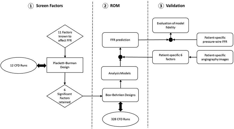
Overall chart describing the method to derive and validate a ROM to calculate FFR.

Screening Factors and RSM

The RSM as a DOE method was used to determine which factors and interaction between factors contributed significantly to FFR. Plackett-Burman method is applied to screen for significant factors; also, the design reduced the computational/experimental effort by eliminating nonsignificant factors. This design is useful for complicated confounding relationship with two-factor interactions. In this study, 11 factors were tested with the Plackett–Burman method (Table 2). The Box-Behnken method as a RSM is an independent quadratic design which is not included in an embedded factorial or fractional factorial method. This design requires three levels of each factor which does contain a center and two levels with the same difference from the center. The Box-Behnken design was then performed with the six factors determined to be significant including stenosis severity ((d-c)*100/d) as shown in Figure 3, diameter of coronary artery, stenosis position (a/b) (Figure 3), volume flow rate, viscosity, and stenosis shape (Table 3). We utilized a previously validated model to calculate volume flow rate [20].FFR is highly complex and based on parameters that involve many factors and interactions. FFR responded nonlinearly to changes in coronary artery diameter and coronary stenosis severity; therefore, coronary diameter and stenosis severity were divided into two sections for each factor. Coronary diameter was tested as either 2-4 mm or 4-6 mm. Coronary stenosis was tested as 40-60% or 60-80%. The four Box–Behnken designs were tested according to Table 2. The ROMswere analysed as a modified model and selected significant two and three factors interaction.

Table 2.

The Plackett–Burman design for 11 factors and its low and high levels

	Factors	Low Level	High Level
A	Pressure (mmHg)	80	140
B	Volume Flow Rate (mL/s)	1	6
C	Stenosis Severity (%)	65	70
D	Length of Stenosis (mm)	10	30
E	Diameter of Artery (mm)	2	6
F	Length of Artery (mm)	30	80
G	Stenosis Position (%)	30	70
H	Stenosis Shape	Eccentric	Concentric
J	Heart Rate	60	140
K	Density (Kg/m3)	1040	1080
L	Viscosity (Kg/m.s)	0.003	0.006

Figure 3.

schematic of different stenosis shapes and different factors.

Table 3.

The Box–Behnken designs for 6 factors and first design (A), second design (B), third design (C) and fourth design (D).

A
	Factors	−1	+1
A	Stenosis Severity (%)	40	60
B	Diameter of Artery (mm)	2	4
C	Stenosis Position (%)	0.25	0.75
D	Volume Flow Rate (mL/s)	1	6
E	Viscosity (Kg/m.s)	0.003	0.006
F	Stenosis Shape	Eccentric	Concentric
B
	Factors	−1	+1
A	Stenosis Severity (%)	60	80
B	Diameter of Artery (mm)	2	4
C	Stenosis Position (%)	0.25	0.75
D	Volume Flow Rate (mL/s)	1	6
E	Viscosity (Kg/m.s)	0.003	0.006
F	Stenosis Shape	Eccentric	Concentric
C
	Factors	−1	+1
A	Stenosis Severity (%)	40	60
B	Diameter of Artery (mm)	4	6
C	Stenosis Position (%)	0.25	0.75
D	Volume Flow Rate (mL/s)	1	6
E	Viscosity (Kg/m.s)	0.003	0.006
F	Stenosis Shape	Eccentric	Concentric
D
	Factors	−1	+1
A	Stenosis Severity (%)	60	80
B	Diameter of Artery (mm)	4	6
C	Stenosis Position (%)	0.25	0.75
D	Volume Flow Rate (mL/s)	1	6
E	Viscosity (Kg/m.s)	0.003	0.006
F	Stenosis Shape	Eccentric	Concentric

CFD Modeling

Blood flow in coronary arteries was simulated using ANSYS Fluent 17.0 and the model validated by Morris, van de Vosse [21]. Blood density was 1,045 kg.m⁻³ for Box-Behnken design [22]. Blood viscosity, a key characteristic for hemodynamic flow modeling, was modeled according to Newtonian viscosity using patient’s measured viscosity [23]. Geometries for RSM, CFD runs were designed in ANSYS Design Modeler. Unstructured computational meshes were built as tetrahedral shaped cells using ICEM CFD 2017. Mesh sensitivity analysis determined an optimal node count for mean residence time quantification for an artery. For Plackett–Burman design, the inlet and outlet boundary conditions were a blood pressure waveform (Figure 2a) and a mass flow rate waveform (Figure 2b) [24]. Both were scaled to match the mean flow in each CFD run, and then programmed using user defined functions (UDF). For Box–Behnken design and patients’ CFD runs, the inlet boundary condition was fixed blood pressure and the outlet boundary condition was fix volume flow rate. Similar to node count, a sensitivity analysis determined an optimal time step size of 0.01s.

Figure 2.

Sample hyperemic boundary conditions: (a) pressure inlet (b) volume flow rate outlet.

Statistical Analysis

The correlation between ROM-FFR and pressure-wire FFR was studied using the Pearson correlation coefficient (r). The patients divided into two groups, abnormal pressure-wire FFR (<=0.80) and normal pressure-wire FFR (>0.80). Receiver operator characteristic (ROC) curve was for ROM-FFR plotted with FFR. A two-sided p-value <0.05 was considered significant. ROM-FFR and FFR were compared using Bland-Altman analysis.

Results

Sceening method Plackett–Burman Design

FFR is the result of a complex interaction between multiple different factors in a myriad of conditions. For this study, 11 major parameters were retained as listed in Table 1. FFR was calculated using CFD and the result of CFD was used as input in each design of experiment. Initially, in order to determine effective factors in calculation of FFR, Plackett–Burman design was used. Placket-Burman reduces the computational/experimental effort by eliminating insignificant factors. Eleven factors along with maximum and minimum values for each factor were selected. Given that stenosis severity (A) is singularly the most important factor in determination of FFR, its range was limited to 65 to 70% and it was included as a highly significant factor in Box–Behnken design for calculation of FFR. The other 10 factors were tested for significance in calculation of FFR through Plackett–Burman design. This analysis indicated that diameter of coronary arteries (B) and volume flow rate (D) at the inlet of coronary segment were the most significant factors affecting FFR and remained significant after application of Bonferroni correction (5.746). Three other factors including shape of stenosis (F), viscosity (E) and stenosis position (C) were also above t-value limit albeit without Bonferroni correction (2.776), hence were selected for Box–Behnken analysis. Based on Plackett–Burman design blood pressure, blood density, length of stenosis, length of coronary segment and heart rate were found to be insignificant factors for FFR calculation.

RSM

In Box-Behnken design, coronary diameter and stenosis severity were divided into two zone: 2-4 mm and 4-6 mm for the former and 40-60% and 60-80% for the latter. This was done in order to enhance the accuracy of the model as the effect of both factors were nonlinear. The result was 4 Box-Behnken design based on the combination of these 2 factors to study the effect of the aforementioned 6 factors in the evaluation of FFR. In the first design, coronary arteries 2 to 4 mm in diameter with stenosis ranging from 40 to 60% were analyzed. Stenosis severity (A), diameter of coronary segment (B), volume flow rate (D), and shape of stenosis (F) and some interactions such as AB, AF, BD, BF, DF, ABF, ADF, BDF were significant for FFR calculation (Table 4). FFR calculation had a significant complexity due to interaction of multiple factors. Figure 4a shows that FFR has an inverse relationship with stenosis severity and direct relation with diameter of coronary artery when stenosis shape is concentric; both were almost linear. On the other hand, for eccentric stenoses (Figure 4b), FFR has a nonlinear relationship with stenosis severity and coronary artery diameter for any artery with a diameter of coronary 2.5 mm. For diameters lower than 2.5 mm, FFR had linear relation with both factors and the relation with diameter of coronary and stenosis is direct and inverse, respectively. Figures 4c and 4d show interaction between diameter of coronary and volume flow rate for concentric and eccentric stenosis and also show how FFR has an inverse relation with volume flow rate and direct relation with diameter.

Table 4.

ANOVA analysis of first design.

Source	Sum of Squares	df	Mean Square	F Value	p-value Prob > F
Model	12.24	22	0.56	53.27	0.0001	significant
A-Stenosis	0.14	1	0.14	13.75	0.0005
B-Diameter of Coronary	2.88	1	2.88	275.96	0.0001
D-Volume Flow Rate	0.39	1	0.39	37.15	0.0001
F-shape	1.17	1	1.17	112.00	0.0001
AB	0.29	1	0.29	27.44	0.0001
AF	0.45	1	0.45	43.05	0.0001
BD	0.85	1	0.85	81.73	0.0001
BF	0.82	1	0.82	78.64	0.0001
DF	0.24	1	0.24	22.54	0.0001
A^2	0.037	1	0.037	3.55	0.0646
B^2	0.80	1	0.80	76.50	0.0001
ABF	0.15	1	0.15	14.59	0.0003
ADF	0.19	1	0.19	18.39	0.0001
BDF	0.17	1	0.17	16.38	0.0002
A^2D	0.071	1	0.071	6.76	0.0117
AB^2	0.13	1	0.13	12.26	0.0009
B^2D	0.26	1	0.26	24.98	0.0001
Residual	0.62	59	0.010
Cor Total	12.86	81
Std. Dev.	0.10	R-Squared	0.9521
Mean	0.72	Adj R-Squared	0.9342

Figure 4.

(a) Interaction AB for concentric and (b) eccentric stenosis and (c) interaction BD for concentric and (d) eccentric stenosis in first design.

In the second design, stenosis, diameter of coronary, position, volume flow rate and shape of stenosis were significant while viscosity was not. AB, AD, AF, BD, BF, CD, CF, DF, ADF, BDF, CDF, A²C, B²C, and C²F were significant (Table 5). The statistical results showed that R-Squared is 0.9395 and the mean and standard deviation was 0.44 and 0.16, respectively. The results could be interpreted that the levels of each factor in the design are so critical for FFR and it is lower than 0.8 with high possibility. The interaction between diameter and stenosis (Figure 5a and 5b) shows that FFR had almost linear relation with diameter of coronary and stenosis. FFR was decreased when diameter decreased, and stenosis increased. Figure 5a confirms that most coronary arteries in range of diameter and stenosis with concentric stenosis may have significant stenosis with high possibility and if the coronary artery had eccentric stenosis (Figure 5b) with diameter of coronary below 2.75 mm it would be significant stenosis. Figures 5c and 5d show interaction between volume flow rate and diameter for concentric and eccentric stenosis. FFR contours changed from linearity to nonlinearity with increasing volume flow rate and decreasing diameter for concentric stenosis whereas, FFR contours changes from linearity to nonlinearity with decreasing volume flow rate and increasing diameter for concentric stenosis. For both concentric and eccentric stenoses, FFR decreases when diameter decreases, and when volume flow rate increases. A coronary artery with a with a diameter of less than 3.2 mm, a concentric stenosis of 60 to 80% is very likely hemodynamically significant (Figure 5c), however, this is only true for coronary arteries smaller than 2.2 mm in diameter with an eccentric stenosis (Figure 5d).

Table 5.

ANOVA analysis for the second design.

Source	Sum of Squares	df	Mean Square	F Value	p-value Prob > F
Model	499.83	25	19.99	34.80	0.0001	significant
A-Stenosis	66.91	1	66.91	116.48	0.0001
B-Diameter of Coronary	82.34	1	82.34	143.34	0.0001
C-Position	14.01	1	14.01	24.39	0.0001
D-Volume Flow Rate	35.12	1	35.12	61.13	0.0001
F-shape	57.73	1	57.73	100.50	0.0001
AB	8.35	1	8.35	14.53	0.0003
AD	9.83	1	9.83	17.11	0.0001
AF	34.61	1	34.61	60.25	0.0001
BD	11.58	1	11.58	20.16	0.0001
BF	30.54	1	30.54	53.16	0.0001
CD	3.63	1	3.63	6.32	0.0149
CF	6.71	1	6.71	11.69	0.0012
DF	27.39	1	27.39	47.69	0.0001
A^2	3.18	1	3.18	5.54	0.0221
B^2	4.89	1	4.89	8.51	0.0051
C^2	3.64	1	3.64	6.33	0.0147
ADF	5.05	1	5.05	8.79	0.0044
BDF	3.61	1	3.61	6.29	0.0151
CDF	3.93	1	3.93	6.83	0.0115
A^2C	5.69	1	5.69	9.90	0.0026
B^2C	5.06	1	5.06	8.80	0.0044
C^2F	3.32	1	3.32	5.78	0.0195
Residual	32.17	56	0.57
Cor Total	532.00	81
Std. Dev.	0.16	R-Squared	0.9395
Mean	0.44	Adj R-Squared	0.9125

Figure 5.

(a) Interaction AB for concentric and (b) eccentric stenosis and (c) interaction BD for concentric and (d) eccentric stenosis in the second design.

In the third design, coronary arteries 4 to 6 mm in diameter with stenosis ranging from 40 to 60% were analyzed. Coronary diameter (B), volume flow rate (D) and shape of stenosis (F) were factors with statistically significant contribution to FFR. Additionally, AC and AF were significant interactions (Table 6). The mean of FFR of 0.96 suggests that with large proximal coronary arteries measuring 4 to 6 mm in diameter and with stenosis in the range of 40 to 60%, no single or combination of the 6 factors above would presumably result in a hemodynamically significant stenosis (Table 5). Figure 6 shows AB and BD interactions in the third design for FFR determination for both concentric and eccentric stenoses and confirms the notion that in coronary arteries with diameter ranging from 4 to 6 mm, coronary stenosis from 40% to 60% is unlikely to be hemodynamically significant.

Table 6.

ANOVA analysis for the third design.

Source	Sum of Squares	df	Mean Square	F Value	p-value Prob > F
Model	0.27	23	0.012	6.52	0.0001	Significant
A-Stenosis	7.133E-003	1	7.133E-003	3.90	0.0529
B-Diameter of Coronary	0.013	1	0.013	7.38	0.0087
D-Volume Flow Rate	0.042	1	0.042	22.98	0.0001
F-shape	0.041	1	0.041	22.65	0.0001
AC	0.018	1	0.018	9.76	0.0028
AF	0.020	1	0.020	10.93	0.0016
DE	0.012	1	0.012	6.35	0.0145
DF	0.018	1	0.018	10.09	0.0024
ACF	0.017	1	0.017	9.57	0.0030
DEF	0.012	1	0.012	6.78	0.0117
A^2C	0.012	1	0.012	6.82	0.0115
AC^2	0.011	1	0.011	6.16	0.0160
Residual	0.11	58	1.827E-003
Cor Total	0.38	81
Std. Dev.	0.043	R-Squared	0.7210
Mean	0.96	Adj R-Squared	0.6103

Figure 6.

(a) Interaction AB for concentric and (b) eccentric stenosis and (c) interaction BD for concentric and (d) eccentric stenosis in third design.

In the fourth design, coronary arteries 4 to 6 mm in diameter with stenosis ranging from 61 to 80% were analyzed. Stenosis severity (A), coronary diameter (B), volume flow rate (D) and shape of stenosis (F) as factors and AB, AD, AF, BD, BF, DF, ABF, A²B, A²D, A²F and AB² as interaction were statistically significant (Table 7). Figure 7 shows AB and BD interactions; FFR contours suggest that these interactions are almost linear for concentric stenosis and nonlinear for eccentric stenosis. Figure 7a suggests that for concentric stenosis of coronary arteries ranging from 4 to 6 mm, the threshold for hemodynamically significant stenosis is between 65 to 75%. For example, FFR is 0.79 in an artery with a diameter of 5 mm and a concentric stenosis of 67% while FFR dramatically drops to 0.37 for the same artery when the stenosis increases to 77%. Figure 7b notably indicated that eccentric stenosis in coronary arteries with diameters ranging from 4 to 6 mm is frequently not hemodynamically significant even when the stenosis severity approaches 80%. Similarly, while increasing volume flow rate in coronary arteries measuring 4 to 6 mm with concentric stenosis ranging from 61 to 80% would result in reduction in FFR, the same is not true about similar arteries with eccentric stenosis where FFR would largely remain above 0.8 (figures 7c and 7d).

Table 7.

ANOVA analysis for the fourth design.

Source	Sum of Squares	df	Mean Square	F Value	p-value Prob > F
Model	8.88	22	0.40	29.45	0.0001	significant
A-Stenosis	1.01	1	1.01	73.89	0.0001
B-Diameter of Coronary	0.17	1	0.17	12.73	0.0007
D-Volume Flow Rate	0.44	1	0.44	31.78	0.0001
F-shape	0.46	1	0.46	33.78	0.0001
AB	0.27	1	0.27	19.96	0.0001
AD	0.36	1	0.36	26.40	0.0001
AF	1.10	1	1.10	80.48	0.0001
BD	0.073	1	0.073	5.30	0.0249
BF	0.23	1	0.23	16.99	0.0001
DF	0.49	1	0.49	35.96	0.0001
A^2	0.55	1	0.55	40.10	0.0001
B^2	0.028	1	0.028	2.02	0.1610
ABF	0.18	1	0.18	13.34	0.0006
A^2B	0.11	1	0.11	8.31	0.0055
A^2D	0.093	1	0.093	6.82	0.0114
A^2F	0.40	1	0.40	28.87	0.0001
Residual	0.81	59	0.014
Cor Total	9.69	81
Std. Dev.	0.12	R-Squared	0.9165
Mean	0.80	Adj R-Squared	0.8854

Figure 7.

(a) Interaction AB for concentric and (b) eccentric stenosis and (c) interaction BD for concentric and (d) eccentric stenosis in the fourth design.

Clinical Validation

FFR based on the above 4 designs was determined in 100 coronary arteries for which the gold standard pressure-wire FFR was known and the correlation between ROM-FFR and pressure-wire FFR was determined. There is a strong correlation between pressure-wire FFR and ROM-FFR (r=0.87, P< 0.001). There were 42 true negatives, 53 true positives, 5 false negative (5%) and, 0 false positives (0%) (Figure 8a). ROM-FFR derived from this model had a sensitivity of 89.4%, specificity of 100% and area under curve of 0.947 (p < 0.05) (Figure 8b). Figure 8c presents a Bland-Altman plot for ROM-FFR and pressure-wire FFR. The Bland-Altman analysis evaluated a bias between the mean differences and estimated an excellent agreement interval, within which 95% of the differences between ROM-FFR and pressure-wire FFR.

Figure 8.

(a) ROM-FFR and pressure-wire FFR for 100 coronary arteries, (b) Receiver operator characteristic (ROC) curve analysis for predicted-FFR against pressure-wire FFR (area under curve=0.947), (c) Bland-Altman analysis, and (d) visualization of ROM-FFR for patient A with FFR 0.9 and patient B with FFR 0.62.

Discussion

In this study, we realized the first comprehensive study of the 11 factors commonly known to affect FFR. Using RSM in conjunction with CFD, we identified 6 factors among the 11 that actually have a significant impact on FFR value: stenosis severity, diameter of coronary arteries, volume flow rate, shape of stenosis, blood viscosity, and stenosis position. Then, using Box–Behnken Design, we establish ROMwhich provide a relation between these significant factors such that FFR could be calculated instantly once these parameters are available without requiring time-consuming CFD-based computation. The ROM was validated by calculating ROM-FFR in 100 stenotic coronary arteries with known pressure-wire FFR. Model predicted-FFR had a sensitivity of 89.4%, specificity of 100% and area under curve of 0.947 (p < 0.05) when compared to pressure-wire FFR. These AUC, sensitivity, and specificity values were generally higher than various forms of computed FFR.

Measurement of pressure-wire FFR is recommended in patients with symptomatic coronary artery disease with intermediate coronary stenosis. Risk of complications, radiation and contrast exposure, procedural time and cost, however, remain of concern. Alternate approaches combining angiography images and CFD have been establish, but CFD run time range (2 hours-5 minutes) is very high for practical use in a clinical setup [21, 25]. In this study, FFR calculated through RSMs had a high degree of agreement in comparison to pressure-wire FFR using standard techniques with significance threshold of 0.80. Indeed, the classification agreement of coronary stenotic lesions was 95% between pressure-wire FFR and predicted-FFR. Although processing times of CFD algorithms vary with their complexity, and usually amount to several hours [8, 25], ROM based RSMs can be used to perform FFR calculations, virtually without delay. Short calculation times allow for real-time use of this method by interventional cardiologists.

Our current study findings provide further clues as to how the clinical and angiographic features of a coronary stenosis affect the FFR value. The most important factors affecting FFR included stenosis severity, coronary artery diameter, blood volume flow rate in coronary arteries and shape of stenosis. There were significant interactions that influenced FFR, the most important of which were interactions between stenosis severity and the shape of stenosis (AF), coronary artery diameter and the shape of stenosis (BF) and blood volume flow rate and the shape of stenosis (DF). It is important to note that the common factor between all these interactions is the shape of stenosis (concentric vs. eccentric). Generally, concentric stenoses were more hemodynamically significant than eccentric stenoses when stenosis severity was identical [26]. From the standpoint of fluid dynamics, this is because blood has to pass through concentric stenosis with a throat that has two sides with significant pressure drop however, when blood passes through eccentric stenosis where presence of a wall side would make it easier for blood to pass through. Notably, the third design suggested that in large coronary arteries with stenosis from 40 to 60% the stenosis is rarely hemodynamically significant.

Previous investigators have used angiography-derived anatomic models to compute FFR. For example, Morris, Ryan [10] used 3D reconstructions obtained by coronary angiography in 19 patients to obtain “virtual FFR” in 30 lesions. They found a correlation between modeled and measured FFR of 0.84 and sensitivity and specificity were reported at 71% and 100% respectively. In a trial of 120 patients, [9] reported an accuracy of 87% for agreement between pressure-wire FFR and a “virtual Functional Assessment Index (vFAI)”. Interestingly, they adjusted the threshold of virtual Functional Assessment Index to 0.82. They reported a sensitivity of 90.4% and specificity of 86.2%. Their accuracy and correlation between simulated and measured FFR (r =0.78) were lower than our method, potentially because they used a standard reference BP of 100 mm Hg and did not incorporate patient-specific values. vFAI was computed in 7 min, based on the distal pressure-to-proximal pressure ratios over the lesion for flows in the range of 0 to 4 ml/s, normalized by the ratio over this range for a normal artery. Tu, Barbato [27] reported a correlation of 0.81 between invasive and modeled vFFR, with sensitivity of 78%, specificity of 93%, and an area under the receiver operating characteristic curve of 0.93 to predict “functionally relevant” lesions by combining quantitative coronary angiography and Thrombolysis In Myocardial Infarction (TIMI) frame count to model coronary flow in 77 vessels in 68 patients. Finally, there are initial data (in 20 patients) regarding CFD modeling on the basis of optical coherence tomography derived 3D anatomy of coronary lesions [27]. More recently, Tu et al. [11] described a method for computing adenosine-flow quantitative flow ratio (QFR). Compared with pressure-wire FFR, aQFR identified physiological lesion significance with sensitivity of 77% and specificity of 89% [11]. Our results indicate that on a per-lesion basis, FFR derived from a ROM demonstrates comparable correlation with pressure-wire FFR in the detection of hemodynamically significant coronary stenosis.

Conclusion

Our study demonstrates that ROM can be used to reliably calculate FFR in patients with intermediate coronary stenosis. This is significant since these ROM can replace time-consuming CFD-based FFR estimation and provide instead a real-time calculation method. By overcoming complexity and time related barriers of CFD, model-based FFR calculation can become a sustainable alternative to the invasive pressure-wire method which is currently the gold standard. In future advancement, a software package can be developed for automatically extracting required parameters from angiography images then computing FFR with the proposed model with minimum human intervention. This would make the application of the propsoed approach practical for widespread clinical use. This method can also be used CT-images for non-invasive determination of FFR.

Highlights.

• The ROM can be used to reliably calculate FFR in patients with intermediate coronary stenosis.

• The ROM can replace time-consuming CFD-based FFR estimation and provide instead a real-time calculation method,

• The ROM-FFR is validated against in One hundred arteries from ninety patients who had undergone FFR measurements.

References

- 1.Pijls NH, et al. , Percutaneous coronary intervention of functionally nonsignificant stenosis: 5-year follow-up of the DEFER Study. Journal of the American College of Cardiology, 2007. 49(21): p. 2105–2111. [DOI] [PubMed] [Google Scholar]
- 2.Pijls NH, et al. , Measurement of fractional flow reserve to assess the functional severity of coronary-artery stenoses. New England Journal of Medicine, 1996. 334(26): p. 1703–1708. [DOI] [PubMed] [Google Scholar]
- 3.Tanaka N, et al. , Coronary flow-pressure relationship distal to epicardial stenosis. Circulation journal, 2003. 67(6): p. 525–529. [DOI] [PubMed] [Google Scholar]
- 4.Boden WE, et al. , Optimal medical therapy with or without PCI for stable coronary disease. New England journal of medicine, 2007. 356(15): p. 1503–1516. [DOI] [PubMed] [Google Scholar]
- 5.Nørgaard BL, et al. , Diagnostic performance of noninvasive fractional flow reserve derived from coronary computed tomography angiography in suspected coronary artery disease: the NXT trial (Analysis of Coronary Blood Flow Using CT Angiography: Next Steps). Journal of the American College of Cardiology, 2014. 63(12): p. 1145–1155. [DOI] [PubMed] [Google Scholar]
- 6.Strisciuglio T and Barbato E, The fractional flow reserve gray zone has never been so narrow. Key Leaders' Opinions on Hot Issues of Cardiovasology, 2016: p. 160. [DOI] [PMC free article] [PubMed] [Google Scholar]
- 7.Taylor CA, Fonte TA, and Min JK, Computational fluid dynamics applied to cardiac computed tomography for noninvasive quantification of fractional flow reserve: scientific basis. Journal of the American College of Cardiology, 2013. 61(22): p. 2233–2241. [DOI] [PubMed] [Google Scholar]
- 8.Min JK, et al. , Noninvasive fractional flow reserve derived from coronary CT angiography: clinical data and scientific principles. JACC: Cardiovascular Imaging, 2015. 8(10): p. 1209–1222. [DOI] [PubMed] [Google Scholar]
- 9.Papafaklis MI, et al. , Fast virtual functional assessment of intermediate coronary lesions using routine angiographic data and blood flow simulation in humans: comparison with pressure wire-fractional flow reserve. Eurointervention, 2014. 10(5): p. 574–583. [DOI] [PubMed] [Google Scholar]
- 10.Morris PD, et al. , Virtual fractional flow reserve from coronary angiography: modeling the significance of coronary lesions: results from the VIRTU-1 (VIRTUal Fractional Flow Reserve From Coronary Angiography) study. JACC: Cardiovascular Interventions, 2013. 6(2): p. 149–157. [DOI] [PubMed] [Google Scholar]
- 11.Tu S, et al. , Diagnostic accuracy of fast computational approaches to derive fractional flow reserve from diagnostic coronary angiography: the international multicenter FAVOR pilot study. JACC: cardiovascular interventions, 2016. 9(19): p. 2024–2035. [DOI] [PubMed] [Google Scholar]
- 12.Pellicano M, et al. , Validation study of image-based fractional flow reserve during coronary angiography. Circulation: Cardiovascular Interventions, 2017. 10(9): p. e005259. [DOI] [PubMed] [Google Scholar]
- 13.Amsallem D and Farhat C, Stabilization of projection-based reduced-order models. International Journal for Numerical Methods in Engineering, 2012. 91(4): p. 358–377. [Google Scholar]
- 14.Amsallem D, Cortial J, and Farhat C, Towards real-time computational-fluid-dynamics-based aeroelastic computations using a database of reduced-order information. AIAA journal, 2010. 48(9): p. 2029–2037. [Google Scholar]
- 15.Kumari P, et al. , Development of parametric reduced-order model for consequence estimation of rare events. Chemical Engineering Research and Design, 2021. 169: p. 142–152. [Google Scholar]
- 16.Lang Y.-d., et al. , Reduced order model based on principal component analysis for process simulation and optimization. Energy & Fuels, 2009. 23(3): p. 1695–1706. [Google Scholar]
- 17.Kim D, et al. , Development, validation and application of a coupled reduced-order CFD model for building control applications. Building and Environment, 2015. 93: p. 97–111. [Google Scholar]
- 18.Polifke W, Black-box system identification for reduced order model construction. Annals of Nuclear Energy, 2014. 67: p. 109–128 [Google Scholar]
- 19.Li D, et al. , Aeroelastic global structural optimization using an efficient CFD-based reduced order model. Aerospace Science and Technology, 2019. 94: p. 105354. [Google Scholar]
- 20.Hashemi J, Non-invasive detection and assessment of coronary stenosis from blood mean residence times. 2019. [Google Scholar]
- 21.Morris PD, et al. , “Virtual” (computed) fractional flow reserve: current challenges and limitations. JACC: Cardiovascular Interventions, 2015. 8(8): p. 1009–1017. [DOI] [PMC free article] [PubMed] [Google Scholar]
- 22.Jung J, Hassanein A, and Lyczkowski RW, Hemodynamic computation using multiphase flow dynamics in a right coronary artery. Annals of biomedical engineering, 2006. 34(3): p. 393. [DOI] [PubMed] [Google Scholar]
- 23.Arzani A, Accounting for residence-time in blood rheology models: do we really need non-Newtonian blood flow modelling in large arteries? Journal of The Royal Society Interface, 2018. 15(146): p. 20180486. [DOI] [PMC free article] [PubMed] [Google Scholar]
- 24.Davies JE, et al. , Evidence of a dominant backward-propagating "suction" wave responsible for diastolic coronary filling in humans, attenuated in left ventricular hypertrophy. Circulation, 2006. 113(14): p. 1768–78. [DOI] [PubMed] [Google Scholar]
- 25.Min JK, et al. , Diagnostic accuracy of fractional flow reserve from anatomic CT angiography. Jama, 2012. 308(12): p. 1237–1245. [DOI] [PMC free article] [PubMed] [Google Scholar]
- 26.Huo Y, et al. , A validated predictive model of coronary fractional flow reserve. Journal of The Royal Society Interface, 2012. 9(71): p. 1325–1338. [DOI] [PMC free article] [PubMed] [Google Scholar]
- 27.Tu S, et al. , Fractional flow reserve calculation from 3-dimensional quantitative coronary angiography and TiMi frame count: a fast computer model to quantify the functional significance of moderately obstructed coronary arteries. JACC: Cardiovascular Interventions, 2014. 7(7): p. 768–777. [DOI] [PubMed] [Google Scholar]