

Abstract
Absorption has always been an attractive process for removing hydrogen sulfide (H2S). Posing unique properties and promising removal capacity, ionic liquids (ILs) are potential media for H2S capture. Engineering design of such absorption process needs accurate measurements or reliable estimation of the H2S solubility in ILs. Since experimental measurements are time-consuming and expensive, this study utilizes machine learning methods to monitor H2S solubility in fifteen various ILs accurately. Six robust machine learning methods, including adaptive neuro-fuzzy inference system, least-squares support vector machine (LS-SVM), radial basis function, cascade, multilayer perceptron, and generalized regression neural networks, are implemented/compared. A vast experimental databank comprising 792 datasets was utilized. Temperature, pressure, acentric factor, critical pressure, and critical temperature of investigated ILs are the affecting parameters of our models. Sensitivity and statistical error analysis were utilized to assess the performance and accuracy of the proposed models. The calculated solubility data and the derived models were validated using seven statistical criteria. The obtained results showed that the LS-SVM accurately predicts H2S solubility in ILs and possesses R2, RMSE, MSE, RRSE, RAE, MAE, and AARD of 0.99798, 0.01079, 0.00012, 6.35%, 4.35%, 0.0060, and 4.03, respectively. It was found that the H2S solubility adversely relates to the temperature and directly depends on the pressure. Furthermore, the combination of OMIM+ and Tf2N-, i.e., [OMIM][Tf2N] ionic liquid, is the best choice for H2S capture among the investigated absorbents. The H2S solubility in this ionic liquid can reach more than 0.8 in terms of mole fraction.
Subject terms: Chemical engineering, Environmental sciences
Introduction
In the recent century, the need for fossil fuels has risen due to the high levels of energy required for the rapid industrialization of the world1. The extraction of oil and gas from underground fields and their combustion for generating heat/energy2 has undesired environmental effect3 and is accompanied by the production of large amounts of undesired pollutants4–6, mainly carbon monoxide (CO)7, carbon dioxide (CO2)8,9, sulfur dioxide (SO2)10, and hydrogen sulfide (H2S)11,12. The most widely used method for removing these gases is absorption13. The absorption processes can help humans meet environmental standards and attenuate the global warming issue14. Nowadays, the absorption process using alkanolamine- based solvent is one of the most developed and industrially interesting approaches15. However, the loss of mono-ethanolamine, diethanolamine, N-methyl-diethanolamine, and di-isopropanol amine creates environmental problems, and they have also produced some highly corrosive byproducts16,17. As an alternative and promising approach, scientists have investigated ionic liquids (ILs)18–20. Ionic liquids are comprised of cations and anions and have an asymmetric organic cation structure, which results in being liquid at room temperature21. Ionic liquids possess outstanding thermal stability and a superior ability to solve organic and non-organic problems18,19. These features are highly attributed to their cation and anion particles. Cations and anions of ionic liquids can be easily modified to make them suitable for many specific applications19. Furthermore, having an insignificant vapor pressure, ILs have been considered promising candidates for sweetening processes with the minimum environmental effect and solvent loss22. A central factor that must be appraised in gas sweetening processes is the solubility of gases in liquids under various dominated operational conditions23,24. Although many references in the literature have calculated or experimentally obtained the CO2 solubility in ILs16–18,25–27, authentic data representing the H2S solubility in ILs is scarce. Therefore, developing robust predictive models is crucial for precisely and expeditiously estimation of H2S solubility data in various operational conditions. In recent years, numerous investigations have been performed to evaluate gas solubility in different ILs. Shariati and Peters28 implemented the Peng–Robinson (PR) equation of state to obtain the solubility of CHF3 in [C2mim][PF6] under various pressures and temperatures. Kroon et al.29 estimated the solubility of CO2 in different ILs at high pressures less than 100 MPa. Wang et al.30 used the square-well chain fluid equation of state (EoS) to assess several gases’ solubility in ILs. Researchers have used numerous EoSs and methods to evaluate both H2S and CO2 solubility in ILs25,31,32. Nevertheless, none of the above-mentioned approaches could be generalized to different systems. As a result, a range of more general approaches must be applied to forecast gas solubility in ILs. Recently, many intelligent methods, such as artificial neural networks (ANNs)33 have been applied for predicting various properties in chemical engineering, including crstallinity34,35, thermal conductivity36,37, viscosity38, heat capacity39, and solubility of different gases in solutions40,41.
Predication of CO2 solubility in ILs is not an exception, and many soft computing methods have been used for this purpose42,43. In contrast, we found that limited investigations have been done regarding the estimation of H2S solubility in ILs using artificial intelligence (AI) models, and further research activities are needed. In the present work, we implement different intelligence models, including multilayer perceptron neural network (MLPNN), adaptive neuro-fuzzy inference system (ANFIS), least-squares support vector machine (LS-SVM), radial basis function neural network (RBFNN), cascade feedforward neural network (CFFNN), and generalized regression neural network (GRNN) for accurate estimation of the H2S solubility in ILs. For this aim, fifteen ILs under different pressure and temperature conditions are investigated. In addition, the preciseness and reliability of the best method have been compared with the UNIFAC EoS. Several graphical and statistical techniques are used to evaluate the performance of the developed models, and the relevancy factor investigates the effect of each input parameter. Moreover, the trend analysis is carried out to assess the capability of the proposed models in detecting the physical trend between the H2S solubility and different temperatures and pressures. At last, the Leverage approach is made to check the validity of the data and feasible region of the best-proposed model.
Theoretical background
Multilayer perceptron neural network
A feedforward MLPNN has three layers of input, interiors, and output44–46. MLPNN benefits from a unique training approach known as the backpropagation, and the utilized activation functions in this method are non-linear47. The three most common types of activation functions are specified as follows37,48:
| 1 |
| 2 |
| 3 |
Adaptive neuro-fuzzy inference system
A combination of ANN with fuzzy logic will result in the emergence of ANFIS systems. Typically, two common structures for FIS approaches exist: (a) Mamdani et al. and (b) Takagi–Sugeno36,49. What is specific about Mamdani et al. method50 is that a list of if–then rules must be defined for the fuzzy inference system, while the fussy interface proposed by Takagi–Sugeno creates its own rules based on the intrinsic features of the provided experimental data to the modeling endeavor. If the output data is nonlinearly dependent on the input data, Takagi–Sugeno ANFIS method will be more useful. Five distinct layers are a typical architecture for the ANFIS structure51. The Fuzzification layer is the first layer in which the conversion of inputted data into linguistic data occurs. The fuzzification process will be done utilizing the defined membership functions. The second layer is used for the model validation by computing a range of parameters known as the firing strengths. The estimated firing strengths are normalized in the next layer, and the fourth layer is responsible for representing outputs’ linguistic terms. Ultimately, all rules attributed to any individual output are combined in the fifth layer50.
Least square-support vector machine
As a robust method for pattern recognition52 and regression53, the LS-SVM is a widely-used and well-developed method. The SVM formulates the function as is given in Eq. (4).
| 4 |
where the output layer’s transposed vector is denoted by wT, the kernel function and bias are given as φ(x) and b, respectively54,55. The size of the input data set and the output ensemble are the determining factors for the SVM’s dimension. The parameters of w and b are then determined by the cost function, given in Eq. (5)54.
| 5 |
The reliable results are possible to achieve by minimizing the cost function considering the following constraints54:
| 6 |
where the kth inputted data and its corresponding output are shown by xk and yk, respectively. In this formulation, ε stands for the accurateness of the function results, and the maximum acceptable errors are given by and Indicates the slack variable. The deviations from ε are determined by c values.
Radial basis function neural network
RBF neural networks are robust predicting methods that use a simpler structure in comparison to MLP networks, the learning step in them is much faster than the MLP’s learning procedure56. Like major artificial neural networks, RBF has three layers: the input layer, the interior layers, and the result layer. The radial basis function is applied to the nodes of hidden layers. Using a linear optimization mechanism, the RBFNN will return precise results when the least mean square error is achieved. Despite all existing similarities between MLPNN and the RBFNN structures, RBFNN utilizes a complex RBF function for hidden layers36.
Cascade fee-forward neural network
The implemented CFFNN in this study could be contemplated as a type of feedforward neural network where the input neurons are connected to all neurons located in the following layers57,58. A range of various learning algorithms is applied to CFFNN models. As one of the most general formulations, the gradient descent algorithm with the momentum is introduced as follows59:
| 7 |
where the weight of neurons is denoted by , the learning pace is shown by α, and bias and the number of training steps are given by b and i, respectively. In these formulations, the momentum parameter is presented by , and the deviation of outputs from the modeling target is represented by 60. Although the updating algorithm for weight factors (given in Eq. 4) is precise, it is just applicable to a small ensemble of data. The weights updating formulation with two terms (i.e., the formulation without ) is a better choice for modeling of large-scale databanks. Equation (8) shows that the cost function is defined by summation of the square error.
| 8 |
where the target and the output patterns are shown by tp and op. The training procedure will not stop unless a pre-defined desirable sum of square errors is obtained61.
Generalized regression neural network
In utilizing the GRNN predictive method, there is no need for an iterative training process13. Instead, between the output and input vectors, any possible arbitrary functions are approximated. In addition to that, this approach is consistent because as larger datasets are fed to the model, the model return more precise results62. Such as the problems solved by the standard regression methods, the GRNN model is also suitable for predicting variables that are intrinsically continuous62. According to the definition of this method, the best and most accurate result for a dependent variable (y) will be obtained when an independent variable x and the training dataset are given, and the model commences minimizing the mean-squared error for the given x data points62.
Experimental data acquisition and preliminary analysis
Data gathering
In the current study, a collection of 792 datasets regarding to H2S solubility in fifteen different ionic liquids, including [OMIM][Tf2N], [OMIM][PF6], [HMIM][PF6], [BMIM][Tf2N], [HMIM][Tf2N], [EMIM][Tf2N], [HOeMIM][Tf2N], [BMIM][BF4], [BMIM][PF6], [EMIM][PF6], [EMIM][eFAP], [HOeMIM][OTF], [HOeMIM][PF6], [HEMIM][BF4], [EMIM][EtSO4] were assembled (the full form of these ionic liquids are introduced in Table 1). The range of operating conditions, i.e., pressure (P) and temperature (T), ionic liquid inherent characteristics, i.e., critical pressure (Pc), critical temperature (Tc), and the acentric factor (ω) are listed in Tables 1 and 2. The range of absorbed hydrogen sulfide by different ionic liquids as the dependent variable is also reported in Table 1. Indeed, these variables are enough to derive a global model for determining the amount of captured H2S in ILs. The gathered data points were divided into two main subsets, including training (85% of the datasets) and testing (15% of the datasets). These groups have been used in a systematic trial-and-error procedure to find the optimal configuration of the model structures and evaluate their performances.
Table 1.
The range of operating conditions during absorbing H2S molecules by different ionic liquids.
| Ionic liquid (Full name) | Abbreviation | Temperature (K) | Pressure (bar) | Solubility (Mole fraction) | Number of data | References |
|---|---|---|---|---|---|---|
| 1-Ethyl-3-methylimidazolium ethylsulfate | [EMIM][EtSO4] | 303.15–353.15 | 1.14–12.70 | 0.012–0.118 | 36 | 17 |
| 1-Ethyl-3-methylimidazolium hexafluorophosphate | [EMIM][PF6] | 333.15–363.15 | 1.45–19.33 | 0.032–0.359 | 40 | 25 |
| 1-Ethyl-3-methylimidazolium bis(trifluoromethylsulfonyl)imide | [EMIM][Tf2N] | 303.15–353.15 | 1.08–16.86 | 0.049–0.609 | 42 | 25 |
| 1-Ethyl-3-methylimidazolium tris(pentafluoroethyl) trifluorophosphate | [EMIM][eFAP] | 303.15–353.15 | 0.58–19.42 | 0.022–0.592 | 79 | 26 |
| 1-Hexyl-3-methylimidazolium bis(trifluoromethanesulfonyl)imide | [HMIM][Tf2N] | 303.15–353.15 | 0.69–20.17 | 0.029–0.701 | 87 | 16,18 |
| 1-Hexyl-3-methylilmidazolium hexafluorophosphate | [HMIM][PF6] | 303.15–343.15 | 1.11–11.00 | 0.050–0.499 | 67 | 16 |
| 1-Butyl-3-methylimidazolium tetrafluoroborate | [BMIM][BF4] | 303.15–343.15 | 0.61–8.36 | 0.030–0.354 | 42 | 63 |
| 1-Butyl-3-methylimidazolium hexafluorophosphate | [BMIM][PF6] | 298.15–403.15 | 0.69–96.30 | 0.016–0.875 | 81 | 63,64 |
| 1-Butyl-3-methylimidazolium bis(trifluoromethylsulfonyl)imide | [BMIM][Tf2N] | 303.15–343.15 | 0.94–9.16 | 0.051–0.510 | 44 | 63 |
| 1-Octyl-3-methylimidazolium bis(trifluoromethylsulfonyl)imide | [OMIM][Tf2N] | 303.15–353.15 | 0.94–19.12 | 0.063–0.735 | 47 | 18 |
| 1-n-Octyl-3-methylimidazolium hexafluorophosphate | [OMIM][PF6] | 303.15–353.15 | 0.85–19.58 | 0.046–0.697 | 48 | 31 |
| 1-(2-Hydroxyethyl)-3-methylimidazolium bis(trifluoromethylsulfonyl)imide | [HOeMIM][Tf2N] | 303.15–353.15 | 1.56–18.32 | 0.057–0.572 | 41 | 27 |
| 1-(2-Hydroxyethyl)-3-methylimidazolium trifluoromethanesulfonate | [HOeMIM][OTf] | 303.15–353.15 | 1.06–18.39 | 0.035–0.548 | 41 | 27 |
| 1-(2-Hydroxyethyl)-3-methylimidazolium hexafluorophosphate | [HOeMIM][PF6] | 303.15–353.15 | 1.34–16.85 | 0.034–0.462 | 47 | 27 |
| 1-(2-Hydroxyethyl)-3-methylimidazolium tetrafluoroborate | [HEMIM][BF4] | 303.15–353.15 | 1.21–10.66 | 0.020–0.247 | 50 | 23 |
Table 2.
The critical temperature, pressure, and acentric factors of ILs used in this study.
| Abbreviation | Tc (K) | Pc (bar) | ω | References |
|---|---|---|---|---|
| [EMIM][EtSO4] | 1061.1 | 40.4 | 0.3368 | 65 |
| [EMIM][PF6] | 663.5 | 19.5 | 0.6708 | 65 |
| [EMIM][Tf2N] | 1244.9 | 32.6 | 0.1818 | 65 |
| [EMIM][eFAP] | 830. 7 | 100.3 | 1.5099 | 66 |
| [HMIM][Tf2N] | 876.2 | 22.2 | 1.3270 | 65 |
| [HMIM][PF6] | 754.3 | 15.5 | 0.8352 | 65 |
| [BMIM][BF4] | 632.3 | 20.4 | 0.8489 | 65 |
| [BMIM][PF6] | 708.9 | 17.3 | 0.7553 | 65 |
| [BMIM][Tf2N] | 1265 | 27.6 | 0.2656 | 65 |
| [OMIM][PF6] | 800.1 | 14.0 | 0.9069 | 19 |
| [OMIM][Tf2N] | 923.0 | 18.7 | 1.3310 | 65 |
| [HOeMIM][Tf2N] | 1297 | 33.1 | 0.5171 | 27 |
| [HOeMIM][OTf] | 1059.1 | 36.7 | 0.6526 | 27 |
| [HOeMIM][PF6] | 766.9 | 20.2 | 1.0367 | 27 |
| [HEMIM][BF4] | 691.9 | 24.7 | 1.1643 | 67 |
Outlier detection
Outliers are typically an inevitable part of every dataset; therefore, eliminating outliers is extremely important for good quality and reliable modeling. Outliers can drastically plummet the model’s accuracy and robustness. The current study reaps the outstanding rewards of utilizing a combination of Leverage and the Hat matrix methods according to the below equation68:
| 9 |
where X is the matrix of independent variables in the [n × m] shape, i.e., numbers of features × numbers of measurements. The process of outlier detection is done using a William plot. Calculation, normalization, and illustration of residual values with respect to the hat value are performed by developing this plot. Simultaneously, a warning leverage value (H*) is calculated using the following expression69:
| 10 |
Statistical criteria for model assessment
Once the models are developed, the accuracy can be evaluated by various statistical approaches to determine their robustness. In the current investigation, the following criteria were utilized for assessing models’ accuracy70,71:
| 11 |
| 12 |
| 13 |
| 14 |
| 15 |
| 16 |
| 17 |
In these equations, employed for statistical evaluation of the results, and show the experimentally measured and the predicted H2S solubilities, respectively. The notation is the average value of , and N stands for the number of data points.
Result and discussion
Development phase
All considered machine learning mthods72–74 have some parameters that need to be tuned using historical data of a given problem and an optimization algorithm75. This research utilizes 792 experimental data of H2S solubility in fifteen ILs versus pressure, temperature, acentric factor, critical pressure, and temperature. The collected databank was randomly split into 673 training and 119 testing datasets.
In the training stage, a machine learning method receives the numerical values of independent as well as dependent variables, while its parameters are unknown76–78. The intelligent model estimates the H2S solubilities from the available independent variables. The deviation between these estimated values and actual H2S solubilities are then needed to be minimized by an optimization algorithm. Indeed, the optimization algorithm continuously updates the parameters of a machine learning method to converge to this minimum value.
In the testing stage, a trained machine learning method receives the independent variables only and calculates the H2S solubility helping the adjusted parameters. The independent variables and machine learning parameters are known in the testing stage, while the dependent variables are unknown.
The accuracy of all machine learning methods in the training and testing stages has been monitored using different statistical indices [i.e., Eqs. (11–17)]. Then, it is possible to find the best model using the ranking analysis. Figure 1 represents a general flowchart for model development in the present study.
Figure 1.

General sketch for development of the proposed models.
Table 3 shows the complete information about the applied trial-and-error procedure during model development. This table shows the numbers of hidden neurons for the MLPNN, CFFNN, and RBFNN, spread factor for the RBFNN and GRNN, cluster radius for the ANFIS, and kernel type for the LS-SVM model is the deciding features in the trial-and-error analyses. Table 3 also presents the cumulative numbers of the developed model for each machine learning class. Generally, 740 models are developed in this study.
Table 3.
General information about the model development phase.
| Model | Decision features | Range of decision features | Numbers of iteration | Numbers of developed models |
|---|---|---|---|---|
| ANFIS | Cluster radius training algorithm | 0.5–1 (10 values) Backpropagation and hybrid | 10 per cluster radius | 200 |
| LS-SVM | Kernel types | Linear, polynomial, Gaussian | 30 per kernel function | 90 |
| MLPNN | Numbers of hidden neurons | 1–9 (9 values) | 10 per hidden neuron | 90 |
| CFFNN | Numbers of hidden neurons | 1–8 (8 values) | 10 per hidden neuron | 80 |
| RBFNN | Numbers of hidden neurons Spread values | 1–9 (9 values) 10–6-10 (20 values) | 20 per hidden neuron | 180 |
| GRNN | Spread values | 10–6-10 (100 values) | One per spread factor | 100 |
Assessment phase
Statistical analyses
After the model development phase, monitoring their accuracy in the training and testing stages employing various statistical criteria is necessary. In this way, it is possible to find the most accurate model in each class using the ranking analysis. The prediction uncertainty of the most precise model in each category in terms of seven statistical criteria is summarized in Table 4. This table states that the cluster radius of 0.5 and Gaussian kernel are the best features for the ANFIS and LS-SVM paradigms. Furthermore, nine, six, and nine hidden neurons are the best topologies of the MLPNN, CFNN, and RBFNN models. The best spread factor for the RBFNN and GRNN models are 3.1579 and 0.00210, respectively. As this table shows, almost all intelligent models are sufficiently robust for estimating hydrogen sulfide solubility in various ionic liquid media. All models show the R2 values greater than 0.99, apart from RBFNN.
Table 4.
Statistical evaluation of the best selected model in each class.
| Model | Key feature | Stage | AARD% | MAE | RAE% | RRSE% | MSE | RMSE | R2 |
|---|---|---|---|---|---|---|---|---|---|
| ANFIS | Cluster radius = 0.5 | Training | 5.20 | 0.0075 | 5.34 | 6.84 | 0.00014 | 0.01178 | 0.997657 |
| Testing | 4.99 | 0.0075 | 5.93 | 7.62 | 0.00014 | 0.01180 | 0.997105 | ||
| Total | 5.17 | 0.0075 | 5.42 | 6.94 | 0.00014 | 0.01178 | 0.997587 | ||
| LS-SVM | Gaussian kernel | Training | 3.89 | 0.0058 | 4.17 | 6.21 | 0.00011 | 0.01063 | 0.998073 |
| Testing | 4.78 | 0.0070 | 5.45 | 7.26 | 0.00014 | 0.01165 | 0.997427 | ||
| Total | 4.03 | 0.0060 | 4.35 | 6.35 | 0.00012 | 0.01079 | 0.997980 | ||
| MLPNN | 9 hidden neurons | Training | 4.76 | 0.0067 | 4.85 | 6.60 | 0.00013 | 0.01131 | 0.997819 |
| Testing | 3.55 | 0.0067 | 5.01 | 7.38 | 0.00014 | 0.01189 | 0.997363 | ||
| Total | 4.58 | 0.0067 | 4.87 | 6.72 | 0.00013 | 0.01140 | 0.997746 | ||
| CFFNN | 6 hidden neurons | Training | 4.95 | 0.0074 | 5.47 | 7.20 | 0.00014 | 0.01202 | 0.997408 |
| Testing | 5.71 | 0.0069 | 4.33 | 7.26 | 0.00018 | 0.01340 | 0.997475 | ||
| Total | 5.06 | 0.0073 | 5.27 | 7.21 | 0.00015 | 0.01224 | 0.997400 | ||
| GRNN | Spread = 0.00210 | Training | 0.59 | 0.0011 | 0.81 | 2.66 | 0.00002 | 0.00460 | 0.999646 |
| Testing | 25.72 | 0.0478 | 40.10 | 39.23 | 0.00344 | 0.05864 | 0.926456 | ||
| Total | 4.36 | 0.0082 | 5.89 | 13.62 | 0.00053 | 0.02312 | 0.990788 | ||
| RBFNN | 9 hidden neurons, spread = 3.1579 | Training | 33.62 | 0.0469 | 33.62 | 35.99 | 0.00380 | 0.06161 | 0.932988 |
| Testing | 26.51 | 0.0405 | 30.99 | 33.19 | 0.00285 | 0.05340 | 0.943624 | ||
| Total | 32.55 | 0.0460 | 33.22 | 35.61 | 0.00365 | 0.06045 | 0.934448 |
Graphical inspection
Different graphical inspections, such as cross-plot and distribution of residual errors, were performed to illustrate the efficiency of the developed models and compare their performances. Figure 2 shows the cross plots of all the implemented approaches and confirms an excellent agreement between experimental and predicted mole fractions of H2S in ILs due to the concentrated accumulation of the training and testing data around the unit slope line. In addition, the relative deviation of the investigated models from experimental data is depicted in Fig. 3. The error distribution provides a suitable visual comparison between the models’ performances. In this figure, LS-SVM, MLPNN, CFFNN, and ANFIS have small scattering to anticipate H2S solubility in various ILs, while the relative deviation of the training and testing data points for GRNN and RBFNN models exceed 40%. These findings confirm the obtained results in Table 4.
Figure 2.

Cross plots of the best model in each class.
Figure 3.

The relative deviations of the selected models for estimating the H2S solubility.
Ranking analysis
The six models were selected before, and their accuracy in the training and testing stages and over the whole of the database was monitored using seven statistical matrices. It is hard to most accurate one through visual inspection. Therefore, the ranking analysis is employed to do so40. Figure 4 provides the results of model ranking in each stage based on the average values of the seven statistical criteria reported in Table 4. The GRNN model in the learning step is the best model; nevertheless, it shows the worst performance in the testing stage. This sharp contrast between the learning ability and the testing results indicates the overfitting of the GRNN model. On the other hand, the LS-SVM with the second-ranking in the training stage and the first ranks for the testing stage and over the whole database is the best model for predicting H2S solubility in ionic liquid media.
Figure 4.

Developed models ranking based on seven different statistical indices.
According to the results of Fig. 4, the developed predictive models can be summarily ranked in terms of their accuracy as follows: LS-SVM > MLPNN > ANFIS > CFFNN > GRNN > RBFNN.
Figure 5 depicts the performance of different models to predict the experimental data of H2S solubility in [BMIM][Tf2N] ionic liquid versus pressure at 343.15 K. The LS-SVM is the most precise model for estimating the H2S solubility in ionic liquid media.
Figure 5.
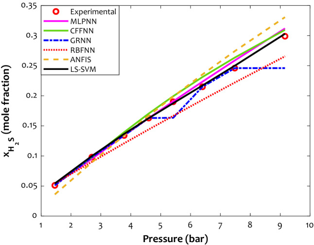
The prediction ability of the developed models for H2S solubility in [BMIM][Tf2N] (T = 343.15 K).
As mentioned earlier, the LS-SVM approach was selected as the best model. In order to better describe the excellent performance of the LS-SVM model, its residual errors (RE) versus the frequency are plotted in Fig. 6. Histograms related to the training, testing, and all data points reveal that the maximum frequency could be seen around residual errors of zero, and virtually all data points are predicted with − 0.05 < RE < + 0.05.
Figure 6.

Histograms of the residual errors (RE) of the LS-SVM for predicting H2S solubility in different IL media (a) training group, (b) testing group, and (c) all datasets.
Equations of state
The prediction uncertainty (in terms of AARD) of the LS-SVM and UNIFAC EoS79 to estimate the 792 collected H2S solubility in various IL media are compared in Fig. 7. It can be seen that the LS-SVM (AARD ~ 14%) and UNIFAC (AARD ~ 30%) show the maximum uncertainty for the H2S solubility in the [HMIM][PF6] ionic liquid. Although the UNIFAC has its second-highest AARD of 27% for [HOeMIM][Tf2N], the obtained value by the LS-SVM is about thirteen times lower (AARD ~ 2%). Indeed, the results predicted by the LS-SVM method are remarkably better than the UNIFAC results. The overall AARD% of UNIFAC for H2S solubility in all IL media is ~ 14%, while it is about 4% for the LS-SVM model. Excluding hydrogen sulfide solubility in the [HMIM][PF6] and [HMIM][TF2N] ionic liquids, the LS-SVM predicts all other systems with the AARD of lower than 5%. It confirms the LS-SVM excellent capability for a wide range of IL/H2S systems.
Figure 7.

Comparison between LS-SVM and UNIFAC uncertainties79 to estimate the H2S solubility in various ILs.
Table 5 presents the accuracy of the proposed LS-SVM model and other approaches reported in the literature based on AARD%. As can be observed, the implemented model in this work shows precise performance for estimating H2S solubility in ILs with AARD% less than that for other EoS models and intelligent algorithms. In addition, other reports have developed for a smaller number of ILs and data points compared to the present study.
Table 5.
Comparison between the developed LS-SVM model and the available approaches in the literature for estimating H2S solubility in ILs based on AARD%.
| Model | No. of data points | No. of ILs | AARD (%) | Ref |
|---|---|---|---|---|
| Peng-Robinson (kij = 0) | 465 | 11 | 38.95 | 80,81 |
| Soave–Redlich–Kwong (kij = 0) | 465 | 11 | 36.43 | 80,81 |
| Peng-Robinson | 465 | 11 | 4.90 | 80,81 |
| Soave–Redlich–Kwong | 465 | 11 | 4.87 | 80,81 |
| Peng-Robinson (kij = 0) | 664 | 14 | 196.76 | 66 |
| Peng-Robinson | 664 | 14 | 8.35 | 66 |
| RETM-CPA | 317 | 5 | 4.41 | 82 |
| SAFT-VR | 225 | 6 | 5.44 | 83 |
| Peng-Robinson-Two State | 636 | 12 | 3.40 | 84 |
| Peng-Robinson (kij = 0) | 664 | 14 | 25.13 | 85 |
| Peng-Robinson | 664 | 14 | 3.67 | 85 |
| FC-ELM | 722 | 16 | 2.33 | 86 |
| Gene expression programming | 465 | 11 | 4.38 | 80,81 |
| MLPNN | 496 | 12 | 1.94 | 87 |
| MLPNN | 664 | 14 | 2.07 | 66 |
| MLPNN | 664 | 13 | 9.08 | 88 |
| RBFNN | 664 | 13 | 26.15 | 88 |
| ANFIS | 664 | 13 | 38.44 | 88 |
| LS-SVM | 792 | 15 | 4.02 | This work |
Relevancy analysis
As stated earlier, the best model was determined LS-SVM with the input parameters, including pressure, temperature, acentric factor, and critical pressure and temperature. In order to study the influence of input parameters on the dissolved mole fraction of H2S in ionic liquids, the relevancy factor was utilized89. This relevancy factor () is defined for all independent variables (i) as follows90:
| 18 |
where ,,, , and represent input parameters, an average of inputs, number of the data points, output parameter, and average of output, respectively. The value of is located within − 1 to 1, and the large values correspond to the strong correlation. Also, the increasing or decreasing of output parameter with variations in attribute to a positive or negative sign, respectively. Two main techniques, namely Spearman and Pearson91, relevancy factors were calculated to ascertain the reliability of the interrelation of the considered independent variables with the H2S solubility as the model's output. According to the results of both methods (Fig. 8), pressure and temperature have the most significant roles in this process, while the acentric factor has the lowest effect. Moreover, it was found that the H2S solubility adversely relates to the temperature and critical pressure of the ionic liquids. Generally, by increasing the pressure, critical temperature, and the acentric factor of ionic liquids, more H2S is expected to be captured.
Figure 8.
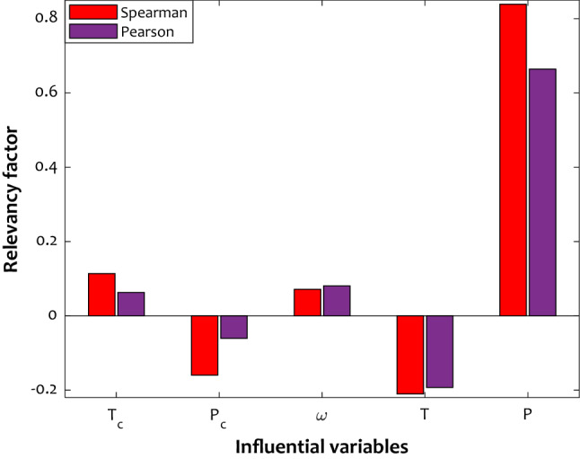
Dependence of H2S solubility in ILs on its influential parameters.
Trend analysis of the LS-SVM
Besides being precise, the developed LS-SVM approach should be able to detect the physical trend of the simulated phenomenon. For doing so, the LS-SVM predictions for H2S solubility in ionic liquids in various temperatures and pressures were compared to the experimentally measured data.
The effect of temperature and pressure
Figure 9 illustrates the solubility of hydrogen sulfide in 1-Butyl-3-methylimidazolium hexafluorophosphate ([BMIM][PF6]) in terms of operating pressure at various temperatures. The H2S solubility in [BMIM] [PF6] was investigated between T = 298.15 K and T = 403.15 K and pressure up to 100 bar. As expected, more H2S molecules dissolved in the [BMIM][PF6] by increasing the operating pressure. However, the H2S solubility in the ionic liquid dramatically decreases as temperature increases. The enhancing effect of pressure is related to the fact that the pressure pushes the H2S molecules into the liquid phase92. Furthermore, this enhancement is more significant in lower pressure. Increasing the kinetic and internal energy of the hydrogen sulfide molecules by increasing the temperature may be responsible for this observation92. Furthermore, dissolving H2S in liquid is an exothermic process. When this gas dissolves in ILs, its molecules interact with ionic liquid molecules and release heat within attractive interaction. Conversely, increasing temperature by adding heat to the solution provides thermal energy that overcomes the attractive forces between the gas and the liquid molecules, thereby decreasing the solubility of the gas.
Figure 9.
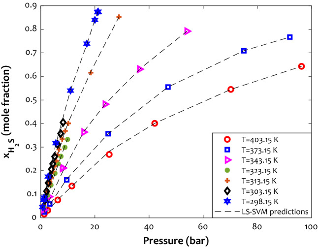
The effect of pressure on the H2S solubility in [BMIM][PF6] ionic liquid in a wide range of temperatures.
The outstanding performance of LS-SVM for predicting the profile and all distinct data points can be concluded from this figure. Indeed, the proposed LS-SVM model successfully understands the influence of operating pressure and temperature on the hydrogen sulfide solubility in the ionic liquid.
The effect of cation and anion type
Assessing the effects of both anions and cations leads to a deep perception of the behavior of H2S solubility in ILs. It is generally found that anions have more influence on the solubility of H2S gas than cations93 As illustrated in Figs. 10a and b, higher H2S solubility was obtained for ILs with the same [TF2N]− anion but higher alkyl chain length ([C8MIM]+ > [C6MIM]+ > [C4MIM]+ > [C2MIM]+ > [C2OHMIM]+). This originates because the longer alkyl chain provides more free volume available in ILs. Aki et al.94 ascribed this behavior to entropic rather than enthalpic reasons, where the molar density of the ILs decreases as the length of the cation alkyl chain gets larger95. As the molar density of the IL decreases, the free volume of the IL enhances the absorption of H2S to occur through a space-filling mechanism96. Consequently, larger free volumes increase H2S solubility by stronger Van der Waals interactions and more H2S molecules absorbed in the solvent23. The above-mentioned trend is an outcome of the variations in molecular interactions of H2S with ionic liquids, which arise from the differences in the chemical constituents, shapes, and sizes of ILs. In addition, H2S solubility for ILs with similar [EMIM]+ but different types of anions was investigated. It was found that higher H2S solubility obtains in anions containing more fluorine content ([TF2N]− > [eFAP]− > [PF6]− > [EtSO4]−), which is in accordance with the other reports in the literature31. Moreover, CO2 and H2S could be strongly attracted in ILs containing [Tf2N]− in compassion with [PF6]−97. As can be seen, the LS-SVM model as a non-linear approach possesses the exceptional capability for estimating the H2S solubility behavior in terms of anion and cation types to obtain reliable quantitative results.
Figure 10.
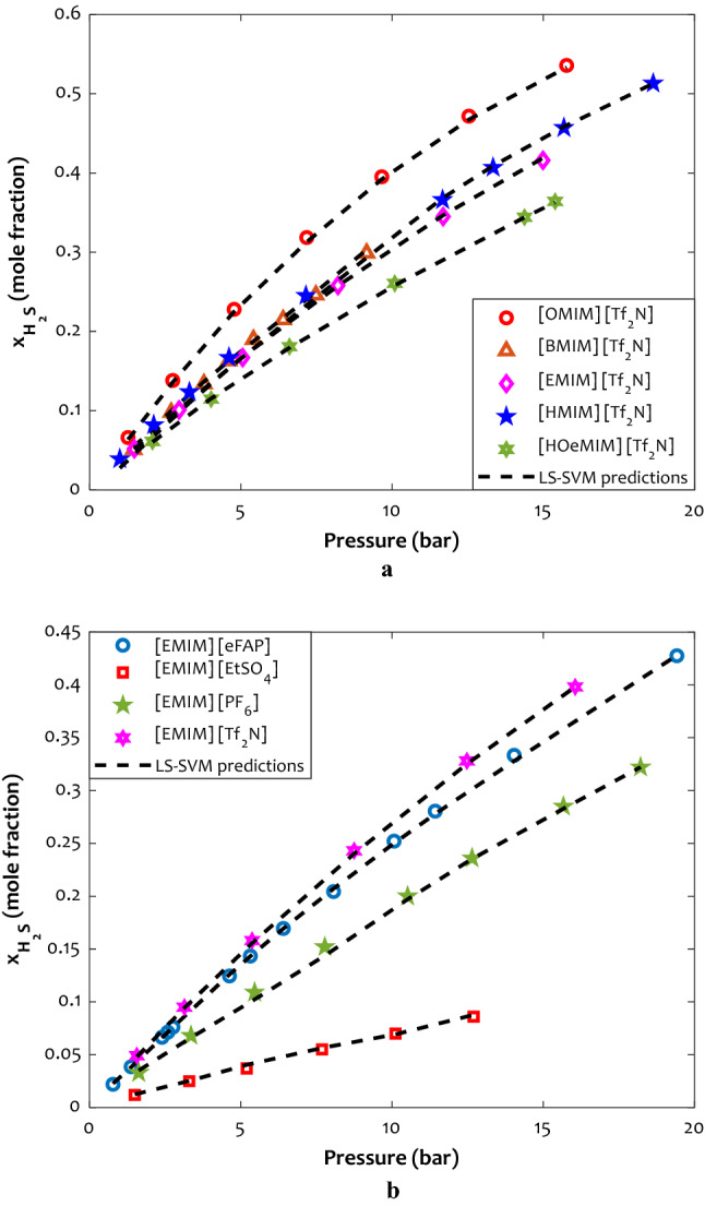
(a) The effect of cation type on the H2S solubility in [Tf2N]-contained ionic liquids (T = 343.15 K) (b) The influence of anion type on the hydrogen sulfide capture ability of the [EMIM]-contained ionic liquids (T = 353.15 K).
The effect of ionic liquid type (cation + anion)
Previous analyses show that the [OMIM]+ and [Tf2N]- provide the highest H2S absorption capacity for the ionic liquid. This section aims to investigate whether their combination poses the highest absorption capacity or not. The effect of absorbent type (combination of cation and anion) on the H2S dissolution in the ionic liquid at the temperature of 333.15 K is depicted in Fig. 11. Generally, an astonishing agreement exists between the calculated hydrogen solubility and the experimentally measured values. As expected, the combination of the [OMIM]+ and [Tf2N]-, i.e., [OMIM][Tf2N] ionic liquid, shows the highest tendency for absorbing the H2S molecules. On the other hand, the [eMIM][EtSO4] is the worst medium for capturing the hydrogen sulfide molecules.
Figure 11.

Comparing the H2S capture tendency of various ionic liquids at T = 333.15 K.
Maximizing H2S solubility in ionic liquid
The previous investigations approved that combining the [OMIM]+ and [Tf2N]-, i.e., [OMIM][Tf2N] ionic liquid synthesized the best medium for absorbing the hydrogen sulfide molecules. This section uses the developed LS-SVM approach to graphically determine the operating condition that maximizes hydrogen sulfide absorption capacity of the [OMIM][Tf2N] ionic liquid. Figure 12 presents pure simulation results for the effect of simultaneous change of pressure and temperature on the H2S solubility in the [OMIM][Tf2N] ionic liquid. It can be seen that increasing the pressure and decreasing the temperature gradually increases the H2S dissolution in the considered ionic liquid. Therefore, the maximum hydrogen solubility of ~ 0.8 is achievable at the highest pressure and lowest temperature.
Figure 12.
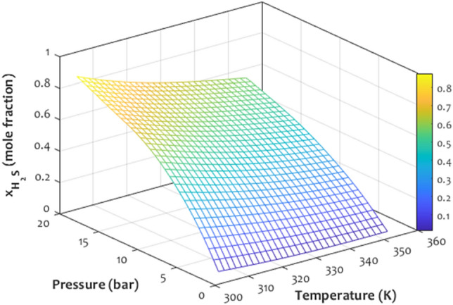
Three-dimensional illustration of temperature and pressure coupled effect on the H2S solubility in [OMIM][Tf2N].
Applicability of LS-SVM and outlier detection
During the model development, standard residuals were calculated and plotted. Data points with standard residuals in the range of − 3 to + 3 (illustrated on the y axis) and Hat indexes limited to 0. The calculated H* (x-axis) values have been recognized as good data points. William’s plot related to the developed LS-SVM model is shown in Fig. 13. As can be seen in this plot, the significant numbers of the point are located in the good Leverage area (0 ≤ H ≤ 0.022 and − 3 ≤ SR ≤ 3)98. Hence, the Leverage approach confirms the validity and reliability of the proposed LS-SVM model for estimating H2S solubility in ILs. Furthermore, the number of outliers is too small to affect the modeling generalization negatively.
Figure 13.
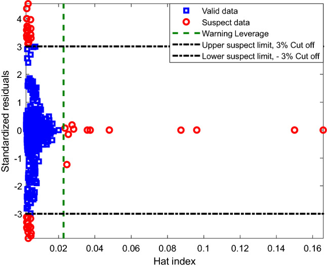
Outlier/valid data detection by the Leverage method.
Application range of the constructed LS-SVM model
Table 1 shows that the H2S solubility data utilized to develop the LS-SVM model are only about imidazole-based ionic liquids containing F atoms. Therefore, this intelligent approach is only valid for the utilized ionic liquids in the reported pressure and temperature ranges.
On the other hand, many different non-F functionalized ionic liquids have also been utilized for H2S absorption. It is possible to collect a databank for H2S solubility in non-F functionalized ionic liquids (or for both F functionalized and non-F functionalized ionic liquids), develop different machine learning methods, compare their accuracy, and find the most accurate model.
Conclusion
The absorption process is likely the most widely used method for H2S removal. Untapped potentials and favorable characteristics of ionic liquids have been enticing for scientists to investigate their H2S removal capacity. However, experimental endeavors are not only costly but time-consuming. On the other hand, since there are many affecting parameters and the interactions between IL and H2S molecules are complex, accurate results cannot be achieved by the equations of state. Fortunately, AI methods can bypass theoretical equations and solve complicated problems expeditiously and accurately. The current study investigated H2S solubility in fifteen ILs by implementing six robust AI methods, including MLPNN, LS-SVM, ANFIS, RBFNN, CFFNN, and GRNN. The temperature, pressure, acentric factor, critical pressure, and critical temperature of investigated ILs are influential variables of the current study. The validation of the derived models was approved using seven statistical criteria. It was found that the LS-SVM was the best predictive model having R2, RMSE, MSE, RRSE, RAE, MAE, and AARD of 0.99798, 0.01079, 0.00012, 6.35%, 4.35%, 0.0060, and 4.03%, respectively. It was found that temperature and the critical pressure of the liquid are adversely related to the H2S solubility. However, the pressure, critical temperature, and acentric factor of ionic liquids increase H2S dissolution in ionic liquids. The outlier detection method justified that a relatively substantial number of data points are valid and have enough quality to be incorporated into the modeling procedure. Finally, the maximum hydrogen solubility of ~ 0.8 is achievable by [OMIM][Tf2N] ionic liquid at the highest pressure and lowest temperature.
Supplementary Information
Acknowledgements
The authors are thankful to the Shahrood University of Technology for the support.
Author contributions
J.A. Writing - Review and Editing, Investigation. M.H. Writing - Review and Editing. SH. EF. Writing - Review and Editing. B.V. Conceptualization, Methodology, Writing - Review and Editing, Resources, Supervision, Validation, Investigation, Resources.
Data availability
A user-friendly and straightforward Matlab-based code has been prepared to use by other research groups (please see Supplementary Information: supplementary_file\Matlab_code). The collected experimental databank has been added to the revised manuscript (please see Supplementary Information: supplementary_file\Database).
Competing interests
The authors declare no competing interests.
Footnotes
Publisher's note
Springer Nature remains neutral with regard to jurisdictional claims in published maps and institutional affiliations.
Supplementary Information
The online version contains supplementary material available at 10.1038/s41598-022-08304-y.
References
- 1.Alizadeh SM, Khodabakhshi A, Hassani PA, Vaferi B. Smart-identification of petroleum reservoir well testing models using deep convolutional neural networks (GoogleNet) ASME J. Energy Resour. Technol. 2021;143:073008. [Google Scholar]
- 2.Lei Z, Yao Y, Yusu W, Yang J, Yuzhen H. Study on denitration performance of MnO2@ CeO2 core-shell catalyst supported on nickel foam. Appl. Phys. A. 2022;128:1–8. [Google Scholar]
- 3.Gong Y, Luo X. Design of Dynamic Diffusion simulation system for atmospheric pollutants in coastal cities under persistent inverse temperature. J. Coast. Res. 2020;103:526–529. [Google Scholar]
- 4.Liu H, et al. Research on the evolution characteristics of oxygen-containing functional groups during the combustion process of the torrefied corn stalk. Biomass and Bioenergy. 2022;158:106343. [Google Scholar]
- 5.Wang S, Zhang L. Water pollution in coal wharfs for coal loading and unloading in coal-fired power plants and its countermeasures. Journal of Coastal Research. 2020;103:496–499. doi: 10.2112/SI103-100.1. [DOI] [Google Scholar]
- 6.Liu J, Zhang Q, Tian X, Hong Y, Nie Y, Su N, et al. Highly efficient photocatalytic degradation of oil pollutants by oxygen deficient SnO2 quantum dots for water remediation. Chem. Eng. J. 2021;404:127146. [Google Scholar]
- 7.Rahimpour MR, Mazinani S, Vaferi B, Baktash MS. Comparison of two different flow types on CO removal along a two-stage hydrogen permselective membrane reactor for methanol synthesis. Appl. Energy. 2011;88:41–51. [Google Scholar]
- 8.Liu W, Zhang Z, Xie X, Yu Z, Von Gadow K, Xu J, et al. Analysis of the global warming potential of biogenic CO2 emission in life cycle assessments. Sci. Rep. 2017;7:1–8. doi: 10.1038/srep39857. [DOI] [PMC free article] [PubMed] [Google Scholar]
- 9.Esmaeili-Faraj SH, Nasr EM. Absorption of hydrogen sulfide and carbon dioxide in water based nanofluids. Ind. Eng. Chem. Res. 2016;55:4682–4690. [Google Scholar]
- 10.Lei, Z., Hao, S., Yusu, W., Yang, J. Study on dry desulfurization performance of MnOx hydrothermally loaded halloysite desulfurizer. Environ. Technol. Innov. 102308 (2022).
- 11.Esmaeili-Faraj SH, Hassanzadeh A, Shakeriankhoo F, Hosseini S, Vaferi B. Diesel fuel desulfurization by alumina/polymer nanocomposite membrane: Experimental analysis and modeling by the response surface methodology. Chem. Eng. Process. Intensif. 2021;164:108396. [Google Scholar]
- 12.Esmaeili Faraj SH, Nasr Esfahany M, Jafari-Asl M, Etesami N. Hydrogen sulfide bubble absorption enhancement in water-based nanofluids. Ind. Eng. Chem. Res. 2014;53:16851–16858. [Google Scholar]
- 13.Zhou Z, Davoudi E, Vaferi B. Monitoring the effect of surface functionalization on the CO2 capture by graphene oxide/methyl diethanolamine nanofluids. J. Environ. Chem. Eng. 2021;9:106202. [Google Scholar]
- 14.Hadipoor M, Keivanimehr F, Baghban A, Ganjali MR, Habibzadeh S. Carbon dioxide as a main source of air pollution: Prospective and current trends to control. Elsevier; 2021. pp. 623–688. [Google Scholar]
- 15.Mousavi NS, Vaferi B, Romero-Martínez A. Prediction of surface tension of various aqueous amine solutions using the unifac model and artificial neural networks. Ind. Eng. Chem. Res. 2021;60:10354–10364. [Google Scholar]
- 16.Rahmati-Rostami M, Ghotbi C, Hosseini-Jenab M, Ahmadi AN, Jalili AH. Solubility of H2S in ionic liquids [hmim][PF6], [hmim][BF4], and [hmim][Tf2N] J. Chem. Thermodyn. 2009;41:1052–1055. [Google Scholar]
- 17.Jalili AH, Mehdizadeh A, Shokouhi M, Ahmadi AN, Hosseini-Jenab M, Fateminassab F. Solubility and diffusion of CO2 and H2S in the ionic liquid 1-ethyl-3-methylimidazolium ethylsulfate. J. Chem. Thermodyn. 2010;42:1298–1303. [Google Scholar]
- 18.Jalili AH, Safavi M, Ghotbi C, Mehdizadeh A, Hosseini-Jenab M, Taghikhani V. Solubility of CO2, H2S, and their mixture in the ionic liquid 1-octyl-3-methylimidazolium bis (trifluoromethyl) sulfonylimide. J. Phys. Chem. B. 2012;116:2758–2774. doi: 10.1021/jp2075572. [DOI] [PubMed] [Google Scholar]
- 19.Shariati A, Ashrafmansouri SS, Osbuei MH, Hooshdaran B. Critical properties and acentric factors of ionic liquids. Korean J. Chem. Eng. 2013;30:187–193. [Google Scholar]
- 20.Marsousi S, Karimi-Sabet J, Moosavian MA, Amini Y. Liquid-liquid extraction of calcium using ionic liquids in spiral microfluidics. Chem. Eng. J. 2019;356:492–505. [Google Scholar]
- 21.Munavirov B, Black JJ, Shah FU, Leckner J, Rutland MW, Harper JB, et al. The effect of anion architecture on the lubrication chemistry of phosphonium orthoborate ionic liquids. Sci. Rep. 2021;11:1–16. doi: 10.1038/s41598-021-02763-5. [DOI] [PMC free article] [PubMed] [Google Scholar]
- 22.Wang L, Xu Y, Li Z, Wei Y, Wei J. CO2/CH4 and H2S/CO2 selectivity by ionic liquids in natural gas sweetening. Energy Fuels. 2018;32:10–23. [Google Scholar]
- 23.Shokouhi M, Adibi M, Jalili AH, Hosseini-Jenab M, Mehdizadeh A. Solubility and diffusion of H2S and CO2 in the ionic liquid 1-(2-hydroxyethyl)-3-methylimidazolium tetrafluoroborate. J. Chem. Eng. Data. 2010;55:1663–1668. [Google Scholar]
- 24.Mohammadi M-R, Hadavimoghaddam F, Pourmahdi M, Atashrouz S, Munir MT, Hemmati-Sarapardeh A, et al. Modeling hydrogen solubility in hydrocarbons using extreme gradient boosting and equations of state. Sci. Rep. 2021;11:1–20. doi: 10.1038/s41598-021-97131-8. [DOI] [PMC free article] [PubMed] [Google Scholar]
- 25.Sakhaeinia H, Jalili AH, Taghikhani V, Safekordi AA. Solubility of H2S in Ionic Liquids 1-Ethyl-3-methylimidazolium Hexafluorophosphate ([emim][PF6]) and 1-Ethyl-3-methylimidazolium Bis (trifluoromethyl) sulfonylimide ([emim][Tf2N]) J. Chem. Eng. Data. 2010;55:5839–5845. [Google Scholar]
- 26.Jalili AH, Shokouhi M, Maurer G, Hosseini-Jenab M. Solubility of CO2 and H2S in the ionic liquid 1-ethyl-3-methylimidazolium tris (pentafluoroethyl) trifluorophosphate. J. Chem. Thermodyn. 2013;67:55–62. [Google Scholar]
- 27.Sakhaeinia H, Taghikhani V, Jalili AH, Mehdizadeh A, Safekordi AA. Solubility of H2S in 1-(2-hydroxyethyl)-3-methylimidazolium ionic liquids with different anions. Fluid Phase Equilib. 2010;298:303–309. [Google Scholar]
- 28.Shariati A, Peters CJ. High-pressure phase behavior of systems with ionic liquids: Part III. The binary system carbon dioxide+ 1-hexyl-3-methylimidazolium hexafluorophosphate. J. Supercrit. Fluids. 2004;30:139–144. [Google Scholar]
- 29.Kroon MC, Karakatsani EK, Economou IG, Witkamp G-J, Peters CJ. Modeling of the carbon dioxide solubility in imidazolium-based ionic liquids with the tPC-PSAFT Equation of State. J. Phys. Chem. B. 2006;110:9262–9269. doi: 10.1021/jp060300o. [DOI] [PubMed] [Google Scholar]
- 30.Wang T, Peng C, Liu H, Hu Y. Description of the pVT behavior of ionic liquids and the solubility of gases in ionic liquids using an equation of state. Fluid Phase Equilib. 2006;250:150–157. [Google Scholar]
- 31.Safavi M, Ghotbi C, Taghikhani V, Jalili AH, Mehdizadeh A. Study of the solubility of CO2, H2S and their mixture in the ionic liquid 1-octyl-3-methylimidazolium hexafluorophosphate: Experimental and modelling. J. Chem. Thermodyn. 2013;65:220–232. [Google Scholar]
- 32.Llovell F, Marcos RM, MacDowell N, Vega LF. Modeling the absorption of weak electrolytes and acid gases with ionic liquids using the soft-SAFT approach. J. Phys. Chem. B. 2012;116:7709–7718. doi: 10.1021/jp303344f. [DOI] [PubMed] [Google Scholar]
- 33.Zhang Z, Tian J, Huang W, Yin L, Zheng W, Liu S. A haze prediction method based on one-dimensional convolutional neural network. Atmos. (Basel) 2021;12:1327. [Google Scholar]
- 34.Ghanbari S, Vaferi B. Prediction of degree of crystallinity for the LTA zeolite using artificial neural networks. Mater. Sci. Pol. 2017;35:486–495. [Google Scholar]
- 35.Wang J, Ayari MA, Khandakar A, Chowdhury MEH, Uz Zaman SM, Rahman T, et al. Estimating the relative crystallinity of biodegradable polylactic acid and polyglycolide polymer composites by machine learning methodologies. Polym. (Basel) 2022;14:527. doi: 10.3390/polym14030527. [DOI] [PMC free article] [PubMed] [Google Scholar]
- 36.Ahmadi MH, Baghban A, Sadeghzadeh M, Hadipoor M, Ghazvini M. Evolving connectionist approaches to compute thermal conductivity of TiO2/water nanofluid. Phys. A Stat. Mech. Appl. 2020;540:122489. [Google Scholar]
- 37.Ahmadi, M.H., Ghazvini, M., Baghban, A., Hadipoor, M., Seifaddini, P., Ramezannezhad, M. et al. Soft computing approaches for thermal conductivity estimation of cnt/water nanofluid. Rev. Des. Compos. Des. Matér. Avancés 29 (2019).
- 38.Çolak, A.B. Analysis of the Effect of arrhenius activation energy and temperature dependent viscosity on non-newtonian maxwell nanofluid bio-convective flow with partial slip by artificial intelligence approach. Chem. Thermodyn. Therm. Anal. 100039 (2022).
- 39.Çolak, A.B. Experimental analysis with specific heat of water-based zirconium oxide nanofluid on the effect of training algorithm on predictive performance of artificial neural network. Heat Transf. Res. 52 (2021).
- 40.Jiang Y, Zhang G, Wang J, Vaferi B. Hydrogen solubility in aromatic/cyclic compounds: prediction by different machine learning techniques. Int. J. Hydrog. Energy. 2021;46:23591–23602. [Google Scholar]
- 41.Xie J, Liu X, Lao X, Vaferi B. Hydrogen solubility in furfural and furfuryl bio-alcohol: comparison between the reliability of intelligent and thermodynamic models. Int. J. Hydrog. Energy. 2021;73:36056–36068. [Google Scholar]
- 42.Torrecilla JS, Palomar J, García J, Rojo E, Rodríguez F. Modelling of carbon dioxide solubility in ionic liquids at sub and supercritical conditions by neural networks and mathematical regressions. Chemom. Syst. Intell. Lab. 2008;93:149–159. [Google Scholar]
- 43.Arce PF, Robles PA, Graber TA, Aznar M. Modeling of high-pressure vapor–liquid equilibrium in ionic liquids+ gas systems using the PRSV equation of state. Fluid Phase Equilib. 2010;295:9–16. [Google Scholar]
- 44.Charandabi SE, Kamyar K. Prediction of cryptocurrency price index using artificial neural networks: a survey of the literature. Eur. J. Bus. Manag. Res. 2021;6:17–20. [Google Scholar]
- 45.Charandabi SE, Kamyar K. Using a feed forward neural network algorithm to predict prices of multiple cryptocurrencies. Eur. J. Bus. Manag. Res. 2021;6:15–19. [Google Scholar]
- 46.Shafiq A, Çolak AB, Sindhu TN. Designing artificial neural network of nanoparticle diameter and solid fluid interfacial layer on SWCNTs/EG nanofluid flow on thin slendering needles. Int. J. Numer. Methods Fluids. 2021 doi: 10.1002/fld.5038. [DOI] [Google Scholar]
- 47.Esmaeili-Faraj SH, Vaferi B, Bolhasani A, Karamian S, Hosseini S, Rashedi R. Design a neuro-based computing paradigm for simulating of industrial olefin plants. Chem. Eng. Technol. 2021;44:1382–1389. [Google Scholar]
- 48.Ghanbari S, Vaferi B. Experimental and theoretical investigation of water removal from DMAZ liquid fuel by an adsorption process. Acta Astronaut. 2015;112:19–28. [Google Scholar]
- 49.Karimi M, Aminzadehsarikhanbeglou E, Vaferi B. Robust intelligent topology for estimation of heat capacity of biochar pyrolysis residues. Measurement. 2021;183:109857. [Google Scholar]
- 50.Ahmadi MH, Baghban A, Ghazvini M, Hadipoor M, Ghasempour R, Nazemzadegan MR. An insight into the prediction of TiO2/water nanofluid viscosity through intelligence schemes. J. Therm. Anal Calorim. 2020;139:2381–2394. [Google Scholar]
- 51.Abd Elaziz M, Moemen YS, Hassanien AE, Xiong S. Quantitative structure-activity relationship model for HCVNS5B inhibitors based on an antlion optimizer-adaptive neuro-fuzzy inference system. Sci. Rep. 2018;8:1–17. doi: 10.1038/s41598-017-19122-y. [DOI] [PMC free article] [PubMed] [Google Scholar]
- 52.Moosavi SR, Vaferi B, Wood DA. Auto-detection interpretation model for horizontal oil wells using pressure transient responses. Adv. Geo-Energy Res. 2020;4:305–316. [Google Scholar]
- 53.Hosseini S, Vaferi B. Determination of methanol loss due to vaporization in gas hydrate inhibition process using intelligent connectionist paradigms. Arab. J. Sci. Eng. 2021 doi: 10.1007/s13369-021-05679-4. [DOI] [Google Scholar]
- 54.Suykens JAK, Van Gestel T, De Brabanter J, De Moor B, Vandewalle J. Least Squares Support Vector Machines. World Scientific Publishing; 2002. [Google Scholar]
- 55.Tang X, Machimura T, Li J, Liu W, Hong H. A novel optimized repeatedly random undersampling for selecting negative samples: a case study in an SVM-based forest fire susceptibility assessment. J. Environ. Manage. 2020;271:111014. doi: 10.1016/j.jenvman.2020.111014. [DOI] [PubMed] [Google Scholar]
- 56.Keshmiri K, Vatanara A, Yamini Y. Development and evaluation of a new semi-empirical model for correlation of drug solubility in supercritical CO2. Fluid Phase Equilib. 2014;363:18–26. [Google Scholar]
- 57.Cao Y, Kamrani E, Mirzaei S, Khandakar A, Vaferi B. Electrical efficiency of the photovoltaic/thermal collectors cooled by nanofluids: Machine learning simulation and optimization by evolutionary algorithm. Energy Rep. 2022;8:24–36. [Google Scholar]
- 58.Alibak, A.H., Khodarahmi, M., Fayyazsanavi, P., Alizadeh, S.M., Hadi, A.J., Aminzadehsarikhanbeglou, E. Simulation the adsorption capacity of polyvinyl alcohol/carboxymethyl cellulose based hydrogels towards methylene blue in aqueous solutions using cascade correlation neural network (CCNN) technique. J. Clean Prod. 130509 (2022).
- 59.Raghuwanshi SK, Pateriya RK. Accelerated singular value decomposition (asvd) using momentum based gradient descent optimization. J. King Saud. Univ. Inf. Sci. 2021;33:447–452. [Google Scholar]
- 60.Zweiri YH, Whidborne JF, Seneviratne LD. A three-term backpropagation algorithm. Neurocomputing. 2003;50:305–318. [Google Scholar]
- 61.Moshkbar-Bakhshayesh K. Development of a modular system for estimating attenuation coefficient of gamma radiation: comparative study of different learning algorithms of cascade feed-forward neural network. J. Instrum. 2019;14:P10010. [Google Scholar]
- 62.Specht DF. A general regression neural network. IEEE Trans. Neural Netw. 1991;2:568–576. doi: 10.1109/72.97934. [DOI] [PubMed] [Google Scholar]
- 63.Jalili AH, Rahmati-Rostami M, Ghotbi C, Hosseini-Jenab M, Ahmadi AN. Solubility of H2S in ionic liquids [bmim][PF6],[bmim][BF4], and [bmim][Tf2N] J. Chem. Eng. Data. 2009;54:1844–1849. [Google Scholar]
- 64.Jou FY, Mather AE. Solubility of hydrogen sulfide in [bmim][PF6] Int. J. Thermophys. 2007;28:490. [Google Scholar]
- 65.Haghbakhsh R, Soleymani H, Raeissi S. A simple correlation to predict high pressure solubility of carbon dioxide in 27 commonly used ionic liquids. J. Supercrit. Fluids. 2013;77:158–166. [Google Scholar]
- 66.Sedghamiz MA, Rasoolzadeh A, Rahimpour MR. The ability of artificial neural network in prediction of the acid gases solubility in different ionic liquids. J CO2 Util. 2015;9:39–47. [Google Scholar]
- 67.Valderrama JO, Rojas RE. Critical properties of ionic liquids Revisited. Ind. Eng. Chem. Res. 2009;48:6890–6900. [Google Scholar]
- 68.Khandelwal M, Kankar PK. Prediction of blast-induced air overpressure using support vector machine. Arab. J. Geosci. 2011;4:427–433. [Google Scholar]
- 69.Moosavi SR, Vaferi B, Wood DA. Auto-characterization of naturally fractured reservoirs drilled by horizontal well using multi-output least squares support vector regression. Arab. J. Geosci. 2021;14:545. [Google Scholar]
- 70.Abdi J, Vossoughi M, Mahmoodi NM, Alemzadeh I. Synthesis of amine-modified zeolitic imidazolate framework-8, ultrasound-assisted dye removal and modeling. Ultrason. Sonochem. 2017;39:550–564. doi: 10.1016/j.ultsonch.2017.04.030. [DOI] [PubMed] [Google Scholar]
- 71.Abdi, J., Hadipoor, M., Hadavimoghaddam, F., Hemmati-Sarapardeh, A. Estimation of tetracycline antibiotic photodegradation from wastewater by heterogeneous metal-organic frameworks photocatalysts. Chemosphere 132135 (2021). [DOI] [PubMed]
- 72.Wu X, Liu Z, Yin L, Zheng W, Song L, Tian J, et al. A haze prediction model in chengdu based on LSTM. Atmos. (Basel) 2021;12:1479. [Google Scholar]
- 73.Yin L, Wang L, Huang W, Liu S, Yang B, Zheng W. Spatiotemporal analysis of haze in Beijing based on the multi-convolution model. Atmos. (Basel) 2021;12:1408. [Google Scholar]
- 74.Azimirad V, Ramezanlou MT, Sotubadi SV, Janabi-Sharifi F. A consecutive hybrid spiking-convolutional (CHSC) neural controller for sequential decision making in robots. Neurocomputing. 2021 doi: 10.1016/j.neucom.2021.11.097. [DOI] [Google Scholar]
- 75.Lin Y, Song H, Ke F, Yan W, Liu Z, Cai F. Optimal caching scheme in D2D networks with multiple robot helpers. Comput. Commun. 2022;181:132–142. [Google Scholar]
- 76.Li Y, Che P, Liu C, Wu D, Du Y. Cross-scene pavement distress detection by a novel transfer learning framework. Comput. Civ. Infrastruct. Eng. 2021;36:1398–1415. [Google Scholar]
- 77.Xu Q, Zeng Y, Tang W, Peng W, Xia T, Li Z, et al. Multi-task joint learning model for segmenting and classifying tongue images using a deep neural network. IEEE J. Biomed. Heal Inf. 2020;24:2481–2489. doi: 10.1109/JBHI.2020.2986376. [DOI] [PubMed] [Google Scholar]
- 78.Azimirad, V., Sotubadi, S.V., Nasirlou, A. Vision-based Learning: a novel machine learning method based on convolutional neural networks and spiking neural networks. In 2021 9th RSI International Conference on Robotics and Mechatronics, IEEE, 192–197 (2021).
- 79.Chen Y, Liu X, Woodley JM, Kontogeorgis GM. Gas Solubility in ionic liquids: UNIFAC-IL model extension. Ind. Eng. Chem. Res. 2020;59:16805–16821. [Google Scholar]
- 80.Ahmadi M-A, Pouladi B, Javvi Y, Alfkhani S, Soleimani R. Connectionist technique estimates H2S solubility in ionic liquids through a low parameter approach. J. Supercrit. Fluids. 2015;97:81–87. [Google Scholar]
- 81.Ahmadi MA, Haghbakhsh R, Soleimani R, Bajestani MB. Estimation of H2S solubility in ionic liquids using a rigorous method. J. Supercrit. Fluids. 2014;92:60–69. [Google Scholar]
- 82.Afsharpour A. Modeling of H2S absorption in some ionic liquids with carboxylate anions using modified HKM plus association EoS together with RETM. Fluid Phase Equilib. 2021;546:113135. [Google Scholar]
- 83.Rahmati-Rostami M, Behzadi B, Ghotbi C. Thermodynamic modeling of hydrogen sulfide solubility in ionic liquids using modified SAFT-VR and PC-SAFT equations of state. Fluid Phase Equilib. 2011;309:179–189. [Google Scholar]
- 84.Shojaeian A. Thermodynamic modeling of solubility of hydrogen sulfide in ionic liquids using Peng Robinson-Two State equation of state. J. Mol. Liq. 2017;229:591–598. [Google Scholar]
- 85.Barati-Harooni A, Najafi-Marghmaleki A, Mohammadi AH. Efficient estimation of acid gases (CO2 and H2S) absorption in ionic liquids. Int. J. Greenh. Gas Control. 2017;63:338–349. [Google Scholar]
- 86.Zhao Y, Gao H, Zhang X, Huang Y, Bao D, Zhang S. Hydrogen sulfide solubility in ionic liquids (ILs): an extensive database and a new ELM model mainly established by imidazolium-based ILs. J Chem. Eng. Data. 2016;61:3970–3978. [Google Scholar]
- 87.Faúndez CA, Fierro EN, Valderrama JO. Solubility of hydrogen sulfide in ionic liquids for gas removal processes using artificial neural networks. J. Environ. Chem. Eng. 2016;4:211–218. [Google Scholar]
- 88.Amedi HR, Baghban A, Ahmadi MA. Evolving machine learning models to predict hydrogen sulfide solubility in the presence of various ionic liquids. J. Mol. Liq. 2016;216:411–422. [Google Scholar]
- 89.Xu J, Liu Z, Yin L, Liu Y, Tian J, Gu Y, et al. Grey Correlation analysis of haze impact factor PM2.5. Atmos. (Basel) 2021;12:1513. [Google Scholar]
- 90.Lashkarbolooki M, Vaferi B, Mowla D. Using artificial neural network to predict the pressure drop in a rotating packed bed. Sep. Sci. Technol. 2012;47:2450–2459. [Google Scholar]
- 91.Karimi M, Vaferi B, Hosseini SH, Olazar M, Rashidi S. Smart computing approach for design and scale-up of conical spouted beds with open-sided draft tubes. Particuology. 2020;55:179–190. [Google Scholar]
- 92.Daryayehsalameh B, Nabavi M, Vaferi B. Modeling of CO2 capture ability of [Bmim][BF4] ionic liquid using connectionist smart paradigms. Environ. Technol. Innov. 2021;22:101484. [Google Scholar]
- 93.Baghban A, Sasanipour J, Habibzadeh S. Estimating solubility of supercritical H2S in ionic liquids through a hybrid LSSVM chemical structure model. Chin. J. Chem. Eng. 2019;27:620–627. [Google Scholar]
- 94.Aki SNVK, Mellein BR, Saurer EM, Brennecke JF. High-pressure phase behavior of carbon dioxide with imidazolium-based ionic liquids. J. Phys. Chem. B. 2004;108:20355–20365. [Google Scholar]
- 95.Fredlake CP, Crosthwaite JM, Hert DG, Aki SNVK, Brennecke JF. Thermophysical properties of imidazolium-based ionic liquids. J. Chem. Eng. Data. 2004;49:954–964. [Google Scholar]
- 96.Blanchard LA, Gu Z, Brennecke JF. High-pressure phase behavior of ionic liquid/CO2 systems. J. Phys. Chem. B. 2001;105:2437–2444. [Google Scholar]
- 97.Anthony JL, Anderson JL, Maginn EJ, Brennecke JF. Anion effects on gas solubility in ionic liquids. J. Phys. Chem. B. 2005;109:6366–6374. doi: 10.1021/jp046404l. [DOI] [PubMed] [Google Scholar]
- 98.Rehamnia I, Benlaoukli B, Jamei M, Karbasi M, Malik A. Simulation of seepage flow through embankment dam by using a novel extended Kalman filter based neural network paradigm: Case study of Fontaine Gazelles Dam, Algeria. Measurement. 2021;176:109219. [Google Scholar]
Associated Data
This section collects any data citations, data availability statements, or supplementary materials included in this article.
Supplementary Materials
Data Availability Statement
A user-friendly and straightforward Matlab-based code has been prepared to use by other research groups (please see Supplementary Information: supplementary_file\Matlab_code). The collected experimental databank has been added to the revised manuscript (please see Supplementary Information: supplementary_file\Database).