

Abstract
A reference interval provides a basis for physicians to determine whether a measurement is typical of a healthy individual. It can be interpreted as a prediction interval for a new individual from the overall population. However, a reference interval based on a single study may not be representative of the broader population. Meta-analysis can provide a general reference interval based on the overall population by combining results from multiple studies. Methods for estimating the reference interval from a random effects meta-analysis have been recently proposed to incorporate the within and between-study variation, but a random effects model may give imprecise estimates of the between-study variation with only few studies. In addition, the normal distribution of underlying study-specific means, and equal within-study variance assumption in these methods may be inappropriate in some settings. In this article, we aim to estimate the reference interval based on the fixed effects model assuming study effects are unrelated, which is useful for a meta-analysis with only a few studies (e.g. ≤ 5). We propose a mixture distribution method only assuming parametric distributions (e.g. normal) for individuals within each study and integrating them to form the overall population distribution. This method is compared to an empirical method only assuming a parametric overall population distribution. Simulation studies have shown that both methods can estimate a reference interval with coverage close to the targeted value (i.e. 95%). Meta-analyses of women daytime urination frequency and frontal subjective postural vertical measurements are reanalyzed to demonstrate the application of our methods.
Keywords: Fixed effects model, meta-analysis, reference interval, very few studies
1. Introduction
In medical sciences, a reference interval is the range of values that is considered normal for a continuous measurement in healthy individuals (for example, the range of blood pressure, or the range of hemoglobin level). We generally expect the measurements of a specified proportion (typically 95%) of a healthy population to fall within this interval. This can also be interpreted as a prediction interval for a measurement from a new healthy individual from the population. Reference intervals are provided for many laboratory measurements and widely used to decide whether an individual is healthy or not. There are two limitations when scientists use the reference interval estimated from a single (particularly small) study for the general population. First, the samples from a single study may not be representative. Second, the reference interval estimated by a small sample size will likely have high uncertainty.1 In some cases, only 20 to 40 individuals in a particular group are available in a study to estimate the reference range, potentially leading to large variations in the resulting upper or lower limits.2 Meta-analysis offers a competitive solution by using samples from multiple studies to establish a reference interval.3–13 The reference interval estimated from a meta-analysis should account for both the within and between-study variation to reflect the distribution of the general population.
The pooled mean has been reported by some meta-analysis studies as a “reference value”, which can only provide information on whether an individual might be above or below the average.10, 11 Although many meta-analysis studies reported the 95% confidence interval (CI) of the pooled mean as the reference interval,4–6, 9 this interval only explains the uncertainty of the pooled mean, not the predicted range for a new individual. Another interval called the “prediction interval” is also commonly reported in some meta-analyses, but it is for predicting the mean of a new study, and does not capture the appropriate range for a new individual.14, 15 This article aims to estimate the reference interval for the overall population to predict the range of measurement of a new individual by synthesizing evidence from multiple studies. We are not interested in predicting the mean of a new study, nor the confidence interval of the pooled mean.
Siegel et al.16 recently proposed a frequentist and a Bayesian method, and an empirical approach for estimating the reference interval from a meta-analysis. However, the frequentist and Bayesian methods, which are based on the random effects model, may lead to inaccurate inference when the number of studies is small (≤ 5).17, 18 Three assumptions are required in the frequentist and Bayesian methods: 1) the normal distribution for individuals within each study, 2) the normality assumption of the underlying study-specific means, and 3) the equal within-study variance across studies. Those assumptions can also be violated. Following the independent parameters assumption in the fixed effects model,19 we propose a mixture distribution method to estimate the reference interval, which may be more suitable when the number studies is small and/or when some assumptions required by the random effects model in Siegel et al.16 are not valid.
In Section 2, we first review the fixed effects meta-analysis. Then, we review the empirical method proposed by Siegel et al.16 which only makes a normal assumption (or more generally a two-parameter exponential family distribution) for the pooled population of all studies. We further extend the fixed effects meta-analysis and proposes the mixture distribution method. The mixture distribution method only makes a distribution assumption for individuals within each study. The simulation in Section 3 shows the performance of the two methods under different data generation processes. We used two real data examples to demonstrate the application of the two methods in Section 4, and a discussion follows in Section 5.
2. Methods
Suppose only the sample size, mean and standard deviation are available for each study. There are three meta-analysis models that can be used, which differ by their between-study heterogeneity assumptions: the common effect model, the fixed effects model and the random effects model.19 The common effect model, also called the fixed effect model, assumes no between-study heterogeneity, and that all studies have the same underlying effect. This model has been criticized for attributing the between-study differences only to the sampling variability.20 The fixed effects model of Laird and Mosteller,20 which is sometimes confused with the common effect model, assumes that the means were separate and fixed with different within-study variances. This model considers the between-study heterogeneity but asserts that the study effects are unrelated. The random effects model assumes the underlying effects in different studies are independent and identically drawn from a single distribution.21 This implies that the study effects are somewhat similar and the similarity is governed by the single distribution.19 The random effects model is frequently chosen if between-study heterogeneity is expected to be present and there is a sufficient number of studies (larger than 5). However, when there are very few studies, the estimate of between-study variance in a random effects model can be highly variable.18 As a typical approach to the random effects model uses the estimated between-study variance to calculate the inverse variance weights to estimate the pooled mean,22 this imprecision may lead to a less desirable estimate of the pooled mean and its confidence interval (CI).23, 24 The imprecise estimate of between-study variance can also lead to inaccurate assessment of the degree of heterogeneity or the degree of similarity across studies. When between-study heterogeneity is expected and only few studies are available, it may be preferable to consider the study-specific effects unrelated and use the fixed effects model. The independent parameters assumption of the fixed effects model implies that the effects of different studies are unrelated, and that they are not random samples from one common distribution like the random effects model.19 Thus, the fixed effects model cannot directly estimate the overall population distribution and make predictions for a new individual from the study-level summary statistics without making some additional assumptions. To address this limitation, we assume the pooled population of the included studies is representative of the overall population. With this assumption, one can estimate the reference range for a new individual from the overall population.
We focus on two methods to combine the results from multiple studies and estimate the pooled population distribution, without making the normality assumption of study-specific underlying means and the equal within-study variance assumption. First, we review and extend the empirical method proposed by Siegel et al.16 which only requires an distributional assumption for an individual in the overall population. We also propose a second method which treats the overall population distribution as a mixture of study-specific distributions, which we call the mixture distribution method. The main difference between the two methods is whether we make a distributional assumption — which can be any distribution completely decided by the mean and variance — for each study or for the overall population. After estimating the overall population distribution, one can use the estimated quantiles to establish the reference intervals. All analyses were performed using R version 4.0.3 (R Core Team), and the R code for real data analysis is provided in the Supplementary Materials.
2.1. The fixed effects model
Let yij denote the j th observation, θi be the underlying true mean, and be the variance for study i = 1, …, k. Typically to estimate a reference range, a parametric (e.g. normal) distribution is assumed within each study. Suppose is the observed mean, ni is the sample size for study i, and ϵi is a random variable describing the sampling error of study i. The fixed effects model is given by
| (1) |
where can be different across studies and the independent parameter assumption is that θi are unrelated. Let μFE be the pooled mean of the overall population in the fixed effects model, and μFE is traditionally estimated as a weighted average of study-specific means:
| (2) |
where can be estimated by the sample variance . The two most commonly used weights are the inverse variance weights proposed by Hedges and Vevea25 and the study sample size weights wi = ni proposed by Hunter and Schmidt26. Marin et al27 found that the sample size weighted average was a practically unbiased estimator while the inverse variance weighted estimated was slightly biased but had the lowest mean squared error. The pooled mean and variance can be used to construct the confidence interval for the pooled mean, but it cannot be used to construct the reference interval predicting the range of the measurement for a new individual from the overall population. We considered the following two methods to estimate the reference interval in a fixed effects meta-analysis.
2.2. The empirical method
The empirical method proposed by Siegel et al16 does not require that the studies have related means or equal within-study variances and therefore can also be used in a fixed effects meta-analysis. This method does not specify the distribution of yij within each study. However, it assumes that the overall population follows a normal distribution, or more generally any distribution completely determined by its mean and variance. The overall mean across all study populations can be estimated by the average of the study means weighted by their study sample sizes:
| (3) |
This is equivalent to the since they use the same weights. Then the marginal variance across studies can be estimated using the conditional variance formula V ar(y) = E[V ar(yij|S = i)] + V ar[E(yij|S = i)]:
| (4) |
where the weights ni − 1 give an unbiased estimate of the variance.16 The limits of the α-level reference interval are then given by the 100 × α/2 and 100 × (1 − α/2) percentiles of a distribution: , where z1−α/2 is the standard normal critical value for the chosen significance level α.
2.3. The mixture distribution method
The mixture distribution method estimates the reference interval by integrating the distribution function constructed by each study mean and variance. The study-specific distribution Fi(y) need to be specified parametrically but there is no need to assume the same parametric distribution for each study, e.g. a normal distribution for all studies. The observations in study i can be assumed to follow any continuous distribution completely determined by the mean θi and variance , such as those from the two parameter-exponential family. The variances can differ across studies. In the fixed effects model, the population mean μFE is estimated by the weighted average of the study-specific means. Similarly, we assume the overall population has a mixture distribution of individual study populations with weight wi:
| (5) |
where F(·) is the cumulative distribution function. For each study, the distribution Fi(y) can be determined approximately by the observed sample mean and sample variance . Then, a 100 × (1 − α)% reference interval, [L,U], based on the pooled population can be estimated by solving the following equations:
| (6) |
where is the estimate of the cumulative distribution function of Fi(y).
When yij can be assumed to be approximately normally distributed, the study-specific cumulative distribution function can be approximately by . When the normality assumption of yij does not hold, another parametric distribution should be used. For example, if the observed measurements have a skewed distribution or when the values cannot be negative, assuming a log-normal distribution where may be more appropriate. In this case, one will need to estimate the mean θi and variance in the log scale from the observed sample mean and sample variance in the original scale as and .28
This mixture distribution method does not require assuming a normal distribution for the overall population but does require a distributional assumption for each study. Moreover, the parametric distributions within each study can be different; we merely use the same distribution in this paper for convenience. We choose the sample sizes as the weights in the mixture distribution method, though other weights such the inverse variance weights can also be used.
3. Simulation
To assess the performance of the mixture distribution method and compare it with the empirical method, we generated the measurements within each study from a normal, a log-normal or a gamma distribution. Following the simulation conducted by Siegel et al,16 the true overall mean μFE was set to be 8 and the total variance was 1.25 for all three distributions. A between-study variance, , was introduced to generate different study-specific means. The true within-study standard deviations were generated from a doubly-truncated normal distribution ϕ(μ = X, σ2 = 1, a = X, b = X + 1), with both the left truncation point and mean equal to X and the right truncation point equal to X + 1, for X ranging from 0 to 0.64, with increments of 0.02. For each X, we estimated by simulating from the doubly-truncated normal distribution. We then set τ2 to be equal to to keep the total variance constant across conditions. Each individual measurement (yij) was simulated from the following full conditional distributions:
| (7) |
where the two parameters in Fi(·) were the means and variances for the normal, log-normal and gamma distributions we assumed. The total number of studies was set to be 2, 5, 10 or 20, with 2 and 5 representing cases with few studies. Each study contained 50 participants. We conducted 1000 simulations for each configuration.
Under each scenario we calculated the fraction of the true population distribution captured by each of the two reference interval methods, which we call the “coverage”. The ratio of between-study variance (τ2) to the total variance and the number of studies k included in the meta-analysis influenced the median coverage and the variation (Figure 1). For normally distributed data in Figure 1a, both the mixture distribution and empirical methods generally had coverages near 95% when the between-study variance was small. The median coverage decreased as the between-study variance increased as a fraction of the total variance; this decrease was most pronounced when k was very small (k = 2). The extreme heterogeneity would be a problem for the case with very few studies. Compared with the empirical method, the median coverage of the mixture distribution method decreased slightly more quickly with the between-study heterogeneity. The variation in coverage increased as the between study heterogeneity τ2 increased and decreased as k increased, while the mixture distribution method had a larger variation than the empirical method. The results for the log-normal distribution are shown in Figure 1b with very similar pattern to the normal distribution. Figure 1c showed that two methods provided almost the same results under a gamma distribution assumption.
Figure 1: Simulation Results:
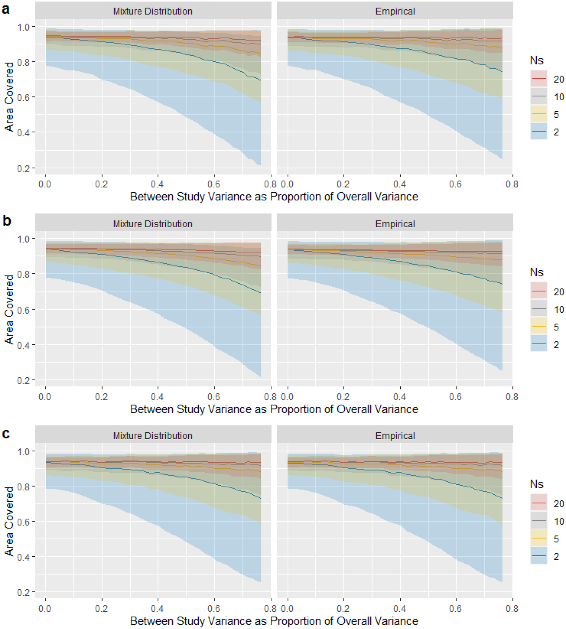
The median (line), 2.5%, and 97.5% (shaded area) of the proportion of the true population distribution captured by the estimated 95% reference interval, for different numbers N of studies. The horizontal axis, proportion of between-study variance to the total variance, represent the degree of heterogeneity across studies. Three distributions are assumed: (a) normal distribution; (b) log-normal distribution; (c) gamma distribution.
4. Two Case Studies
4.1. A meta-analysis of urination frequency during day time
Accurate reference intervals for measurements of bladder function (storage, emptying and bioregulatory) are useful to promote bladder health. They can be used to identify lower urinary tract symptoms and determine whether further evaluation and treatments are needed. Wyman et al7 conducted a meta-analysis with 24 studies to establish normative reference values for bladder function parameters of noninvasive tests in women, including urination frequencies, voided and postvoid residual volumes and uroflowmetry parameters.
Here, we only focused on the daytime urination frequency data which was available in 5 studies to demonstrate our methods with few studies. The high degree of observed heterogeneity across studies, the large I2 value (0.859), and the small number of studies suggest that a fixed effects model is more appropriate than a random effects model. We used the log-normal assumption since the urination frequency data could not be negative and the distribution is skewed. Figure 2 used the urination frequency data to illustrate the mixture distribution method. We first estimated the densities for 5 studies and weighted them by their sample sizes (the blue dashed curves). Then, the 95% reference interval was obtained by letting α = 0.05, which is the region of x-axis between two vertical dashed lines. The solid black curve is the density of the pooled population. Figure 3a shows the means (95% CI) and the prediction interval for a new individual for each study, the 95% CI of the overall mean estimated by the fixed effects model, and the reference intervals based on the methods introduced in Section 2. The overall 95% CI based on the pooled mean gave the narrowest interval ([6.50,6.76]), which represents only the precision in the point estimate. The reference intervals for the empirical method ([3.56,11.32]) and mixture distribution method ([3.53,11.31]) were much wider and overlapped with all studies’ 95% prediction interval. Wyman et al7 used the same mixture distribution method and reported a 90% reference interval [4,10] for the day time urination frequency, and our mixture distribution method had the same result after changing the quantiles to 90%. We also considered a gamma distribution for the measurement in Figure 3b to see the performance of our methods under different distribution assumption. The reference intervals for the empirical method ([3.31,11.09]) and mixture distribution method ([3.29,11.09]) were shifted to the left by 0.2 compared with the results under log-normal assumption. We provided the 95% prediction intervals for a new individual of each study, which is the estimated reference interval if only a single study was available. The prediction intervals for a new observation of each study showed obvious differences representing variation in the study populations. This suggests that a reference interval calculated from a meta-analysis of these studies is more generalizable to the overall population.
Figure 2: An illustration of the 95% reference interval estimated by the mixture distribution method:
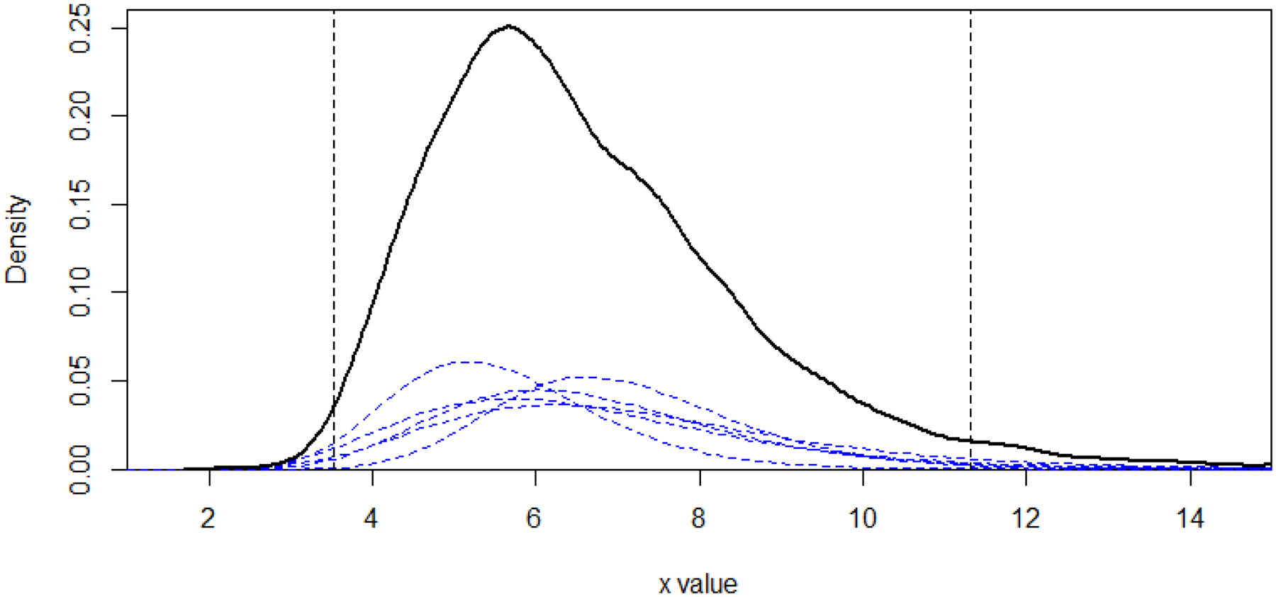
The blue dashed curves are the estimated densities for 5 studies weighted by the sample sizes, and the solid black curve represents the pooled population distribution density. The 95% reference interval is the region of x-axis between two vertical lines, and the sum of area under each blue curve outside the vertical line on each side is equal to 0.025
Figure 3: A Meta-analysis of Daytime Frequency:
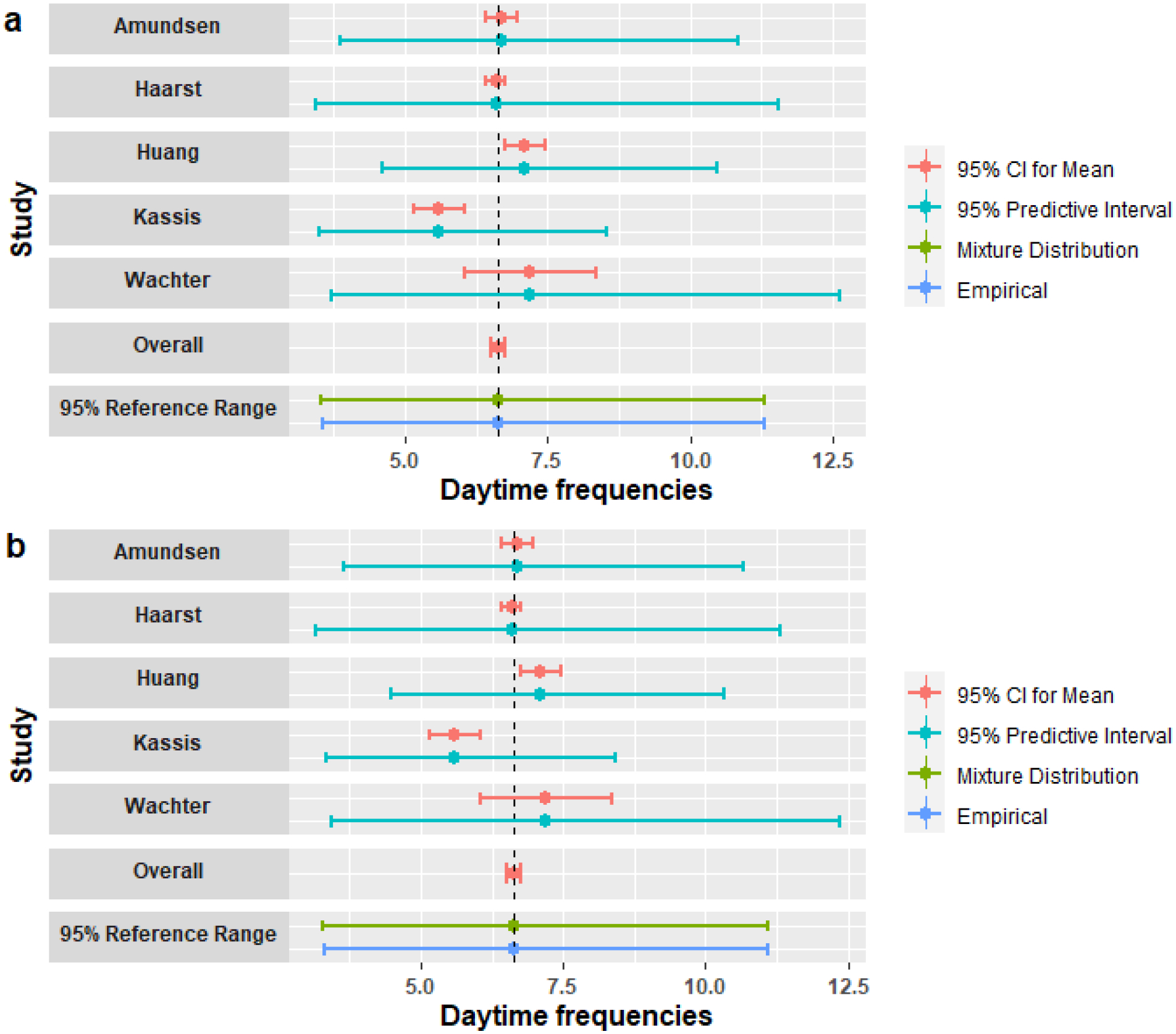
Mean (95% CI) and 95% prediction interval for a new individual for each study; Overall is the 95% CI for pooled mean estimated by the fixed effects model; 95% reference ranges are estimated from the mixture distribution and the empirical methods under: (a) the log-normal distribution; (b) the gamma distribution.
4.2. A meta-analysis of human postural vertical
The second case study is a meta-analysis of human subjective postural vertical (SPV) measurements,12 which reflect an individual’s ability to perceive whether they are vertical or not. Maintaining vertical posture is an important ability when engaging in daily activities.29 Vertical perception is also associated with postural control and functionality and can be altered in stroke patients.30 To measure the SPV, the participants usually sit on a tilting chair with their eyes closed, and verbally instruct an examiner to set the chair to their perceived upright body orientation.
We used the data for frontal SPV from 15 studies that measured the deviation (in degree) of the specified position from true verticality in the frontal planes. This case study was used to demonstrate the application of our methods when the number of studies is relatively large. The meta-analysis included 15 studies measuring frontal SPV and the heterogeneity I2 is 0.909. Conceição et al12 used the empirical method to estimate the pooled mean and standard deviation, then estimated the normal reference interval as . Siegel et al16 proposed the frequentist method and Bayesian method, and estimated the reference intervals as [−2.92, 3.15] and [−3.07, 3.20], respectively. We analyzed the data using the fixed effects model to estimate the pooled mean. As we expected, the 95% CI for the pooled mean was narrow ([−0.04, 0.27]) and did not reflect the variation between individuals. The reference interval calculated using the empirical method was [−2.89, 3.13], the same as Siegel et al’s16 result. Conceição et al’s12 interval was slightly wider since they used 2 times standard deviation instead of 1.96 and weighted by n when estimating the overall variance.12 The mixture distribution method gave a relatively narrower interval [−2.97, 3.10], which was still very close to results of Conceição et al12 and Siegel et al16. Figure 4 shows that the reference intervals estimated using the mixture distribution and empirical methods overlapped with all individual studies’ 95% CIs for the mean, while the 95% CI for the pooled mean only included 4 study means and do not account for the variation. The 95% prediction intervals for a new observation of each study demonstrated a high degree of heterogeneity across studies like the first example. These results reflect how our methods incorporate the full variation in the overall population into the estimated reference intervals.
Figure 4: A Meta-analysis of Sagittal Plane SPV:

Mean (95% CI) and 95% prediction interval for a new individual for each study; Overall is the 95% CI for pooled mean estimated by the fixed effects model; 95% reference ranges are estimated from the mixture distribution and the empirical methods under the normal distribution.
5. Discussion
Meta-analysis is a useful method for synthesizing the results of multiple independent studies to address a particular question. In this paper, we described two methods based on the fixed effects assumption to estimate the normal reference intervals for an individual. One method was a mixture distribution method assuming the overall population distribution is a mixture of individual study distribution. The other method was an empirical method assuming a normal distribution of the overall population.16 The simulation results showed that when using the fixed effects model with a very small number of studies (2 or 5), both methods performed well if the between-study variation was relatively small. However, it is important to consider whether separate results from individual studies would be more informative than a meta-analysis with few studies.18 We recommend choosing the meta-analysis when 1) establishing the reference interval based on the pooled population is necessary, and 2) the estimated between-study variation is no more than 30−50% of the total estimated variation. It may be preferable to calculate separate reference intervals for each study population rather than using a meta-analysis when the number of studies is very small and the heterogeneity between studies is extremely large. The example of frontal SPV demonstrated that the two methods can give very similar reference intervals as the random effects model, when the number of studies is relatively large. It is difficult to predict the study-level mean of a new study or the range of a new individual in a fixed effects model, since the included study effects are assumed unrelated and there is no distribution assumption for the underlying study means. Thus, if the random effects assumption that the underlying study-specific means are from the same distribution is valid, and the number of studies is large, then the between-study variance can be precisely estimated. In this case, the random effects model may be preferred to draw inferences about a hypothetical future study and/or individual not included in the meta-analysis.
The within-study normality assumption in meta-analysis “might not always be appropriate”, especially for small sample size studies or skewed data.17, 31 Log or other transformation can be used for skewed data. If the underlying distribution of the data is not normal and the transformation to a normal population is impossible, the mixture distribution method is still feasible as long as a parametric distribution for each study can be assumed. The empirical method does not make any within-study normality assumption but assumes the overall population follows a known distribution belongs to the two-parameter exponential family. Based on the information obtained from included studies, the choice of the two methods depends on which assumption is more appropriate. In addition to the flexible assumption for the distribution, both methods do not require equal within-study variances.
This paper focuses on the situation that only the study level data is available, making it impossible to avoid making an assumption for within-study distributions or the overall distribution. If the individual patient data (IPD) are available, other methods for estimating the reference intervals for a single study could likely be extended to the meta-analysis setting. For example, nonparametric methods could be used without making assumptions about the specific form of the underlying distribution of the data within each study.2
Finally, it is important to determine whether the studies included in a meta-analysis have reported measurements from the target population whose reference range is being sought. One suggestion is evaluating the inclusion and exclusion criteria of the meta-analysis based on the population of interest. For example, 16 studies were excluded in Conceição et al12 because their SPV protocol was not in seated position or used control groups with non-healthy participants. Furthermore, considering different instruments can be used to get measurements, the reference interval for measurements obtained by one instrument might not be applicable for measurements from other instruments.
Although in this paper we assume that each study reports the sample size, mean and standard deviation (SD) of the outcome, some articles report the sample median, the minimum and maximum values, and/or the first and third quartiles, especially when the data are skewed. Multiple methods have been proposed to estimate the sample mean and SD by using those summary statistics.32–35 With the estimated sample mean and SD, those studies can be included in the meta-analysis. Furthermore, for studies reported those summary statistics in addition to the mean and SD, the quantile-matching estimation (QME) may be used to better estimate the parameters of the within-study distribution.36, 37 While the methods presented in this paper only use aggregated study-level data, future studies may consider estimating the reference interval by combing studies with individual participant data and studies with aggregated study-level data. Future work could also investigate the effect of subject characteristics, such as age, on the normal reference range by incorporating covariates in the meta-regression model. In addition, it may also be fruitful to investigate the impact of small study effects, publication and other biases on the estimation of reference range.38–40
Supplementary Material
Highlights.
What is already known?
A reference interval based on one study can help scientists determine whether the measurement of an individual is normal. This range may not be generalizable to the overall population due to a small sample size.
A 95% confidence interval for the pooled mean should not be reported as a reference interval as it does not incorporate both the between- and within- study variations.
Previous literature gives guidance on how to estimate reference intervals from a random effects meta-analysis, which may not work well for a meta-analysis when only a few studies are available.
What is new?
We present a mixture distribution methods on the fixed effects model assumption to estimate the reference interval for an individual, especially when the number of studies is small. The fixed effects model does not assume equal within-study variances.
The mixture distribution method assumes parametric distributions for individuals within each study, while the empirical method assumes a parametric distribution for the overall population.
Simulation results indicate that the two methods perform similarly. They both tend to underestimate the width of the reference interval when the between-study heterogeneity is large, particularly when the number of studies is small.
When the number of studies is relatively large, the real data example showed that the two methods provide similar results to the random effects models.
Acknowledgements and Funding
This research was funded in part by the U.S. National Institutes of Health’s National Center for Advancing Translational Sciences grant UL1TR002494, National Library of Medicine grant R01LM012982, and NIH National Heart, Lung, and Blood Institute grant T32HL129956.
Footnotes
Conflict of Interest
The author reported no conflict of interest.
Data Availability Statement
The data that support the findings in this study are available in Tables 1 and 2 of the Supplementary Materials.
References
- 1.Horn PS, Pesce AJ. A robust approach to reference interval estimation and evaluation. Clin Chim Acta. 2003;334(1–2):5–23. [PubMed] [Google Scholar]
- 2.Horn PS, Pesce AJ, Copeland BE. A robust approach to reference interval estimation and evaluation. Clin Chem. 1998;44(3):622–631. [PubMed] [Google Scholar]
- 3.Haidich AB. Meta-analysis in medical research. Hippokratia. 2010;14(Suppl 1):29–37. [PMC free article] [PubMed] [Google Scholar]
- 4.Pathan F, D’Elia N, Nolan MT, Marwick TH, Negishi K. Normal ranges of left atrial strain by speckle-tracking echocardiography: a systematic review and meta-analysis. J Am Soc Echocardiogr. 2017;30(1):59–70. [DOI] [PubMed] [Google Scholar]
- 5.Levy PT, Machefsky A, Sanchez AA, et al. Reference ranges of left ventricular strain measures by two-dimensional speckle-tracking echocardiography in children: a systematic review and meta-analysis. J Am Soc Echocardiogr. 2016;29(3):209–225. [DOI] [PMC free article] [PubMed] [Google Scholar]
- 6.Venner AA, Doyle-Baker PK, Lyon ME, Fung TS. A meta-analysis of leptin reference ranges in the healthy paediatric prepubertal population. Ann Clin Biochem. 2009;46(1):65–72. [DOI] [PubMed] [Google Scholar]
- 7.Wyman JF, Zhou J, LaCoursiere DY, et al. Normative noninvasive bladder function measurements in healthy women: a systematic review and meta-analysis. Neurourol Urodyn. 2020;39(2):507–522. [DOI] [PMC free article] [PubMed] [Google Scholar]
- 8.Khoshdel AR, Thakkinstian A, Carney SL, Attia J. Estimation of an age-specific reference interval for pulse wave velocity: a meta-analysis. J Hypertens. 2006;24(7):1231–1237. [DOI] [PubMed] [Google Scholar]
- 9.Bazerbachi F, Haffar S, Wang Z, et al. Range of normal liver stiffness and factors associated with increased stiffness measurements in apparently healthy individuals. Clin Gastroenterol Hepatol. 2019;17(1):54–64. [DOI] [PubMed] [Google Scholar]
- 10.Galland BC, Short MA, Terrill P, et al. Establishing normal values for pediatric night-time sleep measured by actigraphy: a systematic review and meta-analysis. Sleep. 2018;41(4):zsy017. [DOI] [PubMed] [Google Scholar]
- 11.Benfica P, Aguiar LT, Brito S, Bernardino LHN, Teixeira-Salmela LF, Faria C. Reference values for muscle strength: a systematic review with a descriptive meta-analysis. Braz J Phys Ther. 2018;22(5):355–369. [DOI] [PMC free article] [PubMed] [Google Scholar]
- 12.Conceição LB, Baggio JA, Mazin SC, Edwards DJ, Santos TE. Normative data for human postural vertical: a systematic review and meta-analysis. PLoS One. 2018;13(9):e0204122. [DOI] [PMC free article] [PubMed] [Google Scholar]
- 13.Staessen JA, Fagard RH, Lijnen PJ, Thijs L, Van Hoof R, Amery AK. Mean and range of the ambulatory pressure in normotensive subjects from a meta-analysis of 23 studies. Am J Cardiol. 1991;67(8):723–727. [DOI] [PubMed] [Google Scholar]
- 14.IntHout J, Ioannidis JP, Rovers MM, Goeman JJ. Plea for routinely presenting prediction intervals in meta-analysis. BMJ Open. 2016;6(7):e010247. [DOI] [PMC free article] [PubMed] [Google Scholar]
- 15.Chiolero A, Santschi V, Burnand B, Platt RW, Paradis G. Meta-analyses: with confidence or prediction intervals?. Eur J Epidemiol. 2012;27(10):823–825. [DOI] [PubMed] [Google Scholar]
- 16.Siegel L, Murad MH, Chu H. Estimating the Reference Range from a Meta-Analysis. Res Synth Methods. 2021;12(2):148–160. [DOI] [PMC free article] [PubMed] [Google Scholar]
- 17.Jackson D, White IR. When should meta-analysis avoid making hidden normality assumptions?. Biom J. 2018;60(6):1040–1058. [DOI] [PMC free article] [PubMed] [Google Scholar]
- 18.Higgins JP, Thompson SG, Spiegelhalter DJ. A re-evaluation of random-effects meta-analysis. J R Stat Soc Ser A Stat Soc. 2009;172(1):137–159. [DOI] [PMC free article] [PubMed] [Google Scholar]
- 19.Rice K, Higgins JP, Lumley T. A re-evaluation of fixed effect(s) meta-analysis. J R Stat Soc Ser A Stat Soc. 2018;181(1):205–227. [Google Scholar]
- 20.Laird NM, Mosteller F. Some statistical methods for combining experimental results. Int J Technol Assess Health Care. 1990;6(1):5–30. [DOI] [PubMed] [Google Scholar]
- 21.Borenstein M, Hedges LV, Higgins JP, Rothstein HR. A basic introduction to fixed-effect and random-effects models for meta-analysis. Res Synth Methods. 2010;1(2):97–111. [DOI] [PubMed] [Google Scholar]
- 22.DerSimonian R, Laird N. Meta-analysis in clinical trials. Control Clin Trials. 1986;7(3):177–188. [DOI] [PubMed] [Google Scholar]
- 23.Böhning D, Malzahn U, Dietz E, Schlattmann P, Viwatwongkasem C, Biggeri A. Some general points in estimating heterogeneity variance with the DerSimonian–Laird estimator. Biostatistics. 2002;3(4):445–457. [DOI] [PubMed] [Google Scholar]
- 24.Cornell JE, Mulrow CD, Localio R, et al. Random-effects meta-analysis of inconsistent effects: a time for change. Ann Intern Med. 2014;160(4):267–270. [DOI] [PubMed] [Google Scholar]
- 25.Hedges LV, Vevea JL. Fixed- and random-effects models in meta-analysis. Psychol Methods. 1998;3(4):486–504. [Google Scholar]
- 26.Hunter JE, Schmidt FL. Methods of meta-analysis: Correcting error and bias in research findings. 55 City Road, London: SAGE Publications, Ltd; 3rd ed. 2015. [Google Scholar]
- 27.Marín-Martínez F, Sánchez-Meca J. Weighting by inverse variance or by sample size inrandom-effects meta-analysis. Educ Psychol Meas. 2010;70(1):56–73. [Google Scholar]
- 28.Quan H, Zhang J. Estimate of standard deviation for a log-transformed variable using arithmetic means and standard deviations. Stat Med. 2003;22(17):2723–2736. [DOI] [PubMed] [Google Scholar]
- 29.Barra J, Marquer A, Joassin R, et al. Humans use internal models to construct and update a sense of verticality. Brain. 2010;133(12):3552–3563. [DOI] [PubMed] [Google Scholar]
- 30.Pérennou D, Mazibrada G, Chauvineau V, et al. Lateropulsion, pushing and verticality perception in hemisphere stroke: a causal relationship?. Brain. 2008;131(9):2401–2413. [DOI] [PubMed] [Google Scholar]
- 31.Stijnen T, Hamza TH, Özdemir P. Random effects meta-analysis of event outcome in the framework of the generalized linear mixed model with applications in sparse data. Stat Med. 2010;29(29):3046–3067. [DOI] [PubMed] [Google Scholar]
- 32.McGrath S, Zhao X, Steele R, Thombs BD, Benedetti A, Collaboration DSDD. Estimating the sample mean and standard deviation from commonly reported quantiles in meta-analysis. Stat Methods Med Res. 2020;29(9):2520–2537. [DOI] [PMC free article] [PubMed] [Google Scholar]
- 33.Luo D, Wan X, Liu J, Tong T. Optimally estimating the sample mean from the sample size, median, mid-range, and/or mid-quartile range. Stat Methods Med Res. 2018;27(6):1785–1805. [DOI] [PubMed] [Google Scholar]
- 34.Wan X, Wang W, Liu J, Tong T. Estimating the sample mean and standard deviation from the sample size, median, range and/or interquartile range. BMC Med Res Methodol. 2014;14(1):1–13. [DOI] [PMC free article] [PubMed] [Google Scholar]
- 35.Shi J, Luo D, Weng H, et al. Optimally estimating the sample standard deviation from the five-number summary. Res Synth Methods. 2020;11(5):641–654. [DOI] [PubMed] [Google Scholar]
- 36.Dominicy Y, Veredas D. The method of simulated quantiles. J Econom. 2013;172(2):235–247. [Google Scholar]
- 37.Sgouropoulos N, Yao Q, Yastremiz C. Matching a distribution by matching quantiles estimation. J Am Stat Assoc. 2015;110(510):742–759. [DOI] [PMC free article] [PubMed] [Google Scholar]
- 38.Lin L, Chu H, Murad MH, et al. Empirical comparison of publication bias tests in meta-analysis. J Gen Intern Med. 2018;33(8):1260–1267. [DOI] [PMC free article] [PubMed] [Google Scholar]
- 39.Lin L, Chu H. Quantifying publication bias in meta-analysis. Biometrics. 2018;74(3):785–794. [DOI] [PMC free article] [PubMed] [Google Scholar]
- 40.Lin L, Shi L, Chu H, Murad MH. The magnitude of small-study effects in the Cochrane Database of Systematic Reviews: an empirical study of nearly 30,000 meta-analyses. BMJ Evid Based Med. 2020;25(1):27–32. [DOI] [PMC free article] [PubMed] [Google Scholar]
Associated Data
This section collects any data citations, data availability statements, or supplementary materials included in this article.
Supplementary Materials
Data Availability Statement
The data that support the findings in this study are available in Tables 1 and 2 of the Supplementary Materials.