Abstract
The forecasting of the nature and dynamics of emerging coronavirus (COVID-19) pandemic has gained a great concern for health care organizations and governments. The efforts aim to to suppress the rapid and global spread of its tentacles and also control the infection with the limited available resources. The aim of this work is to employ real data set to propose and analyze a compartmental discrete time COVID-19 pandemic model with non-linear incidence and hence predict and control its outbreak through dynamical research. The Basic Reproduction Number () is calculated analytically to study the disease-free steady state (), and also the permanency case () of the disease. Numerical results show that the transmission rates and are quite effective in reducing the COVID-19 infections in India or any country. The fitting and predictive capability of the proposed discrete-time system are presented for relishing the effect of disease through stability analysis using real data sets.
Introduction
Today, the daily life of the human population starts with the concern of fighting against the pandemic COVID-19 outbreak cited by Choi et al. [9] and Gralinski and Menachery [17]. It is reported that COVID-19 virus can transmit from infected individual to susceptible one through a direct contact with respiratory droplets caused by coughing or sneezing. Although coronavirus can survive on surfaces for several hours, it is found that conventional disinfectants can eliminate it. The ways and mechanisms by which COVID-19 affects people gains a lot of attentions, see for example Huang et al. [21], Cheng and Shan [8], Gralinski and Menachery [17], Chen et al. [7]. It has been observed that older people and individuals having chronic medical conditions are more risk of developing severe symptoms when infected by the COVID-19. Although, there are relatively fewer cases of COVID-19 among children, individuals of any age can get infected by the virus.
The main aim of the proposed discrete-time model is to realize the effect of disease due to coronavirus and find all the characteristics which are liable for this outbreak of respiratory illness. The discrete time models provide more appropriate tools for describing processes having different scales of time or which evolve over non-overlapping intervals. In addition, employing discrete models results in a significant reduction in computational complexity of the associated continuous time models. Thus, mathematical modeling and study of nonlinear maps can be advantageously [2, 4, 13]. The non-linear incidence rate are used in epidemic models to provide more accurate modeling of the disease spread rate [15, 24, 26, 28]. Wesley et al. [27] presented a discrete-time rodent-hantavirus model structured by infection and developmental stages. The differences between the dynamics of the male and female rodents in deterministic and stochastic versions of the model are investigated using numerical simulations. Hernandez et al. [19] studied the epidemic maps when arbitrary stage distributions were considered and also the potential applications to disease control were investigated. The analytical and numerical results of this model clarified the inconsistencies in forecasting which arise due to the employment of specific parametric distributions. The quarantine or isolation, among other control measures, are utilized to control the reproduction number and drive the final epidemic size to a predetermined value. Biswas et al. [5] presented an SEIR Model and studied control the infectious Diseases with constraints. Different models for the COVID-19 pandemic have been proposed and analyzed in literature. Huang and Qiao [20] presented the characteristics of the epidemic dynamics through data-driven time-dependent transmission rate for the COVID-19.
The paper discusses the equilibrium points of the proposed discrete-time model of COVID-19 and their stability analysis. The basic reproduction number for the proposed discrete-time COVID-19 model is obtained using the next-generation matrix method. The values of parameters in the model are estimated by fitting realistic data sets. The numerical analysis with a brief discussion and conclusion have been presented incorporating spreading and transmission dynamics of COVID-19.
Description of discrete-time COVID-19 model
In the past 50 years, many researchers have formulated a plethora of mathematical models of the spread of infectious diseases in human populations. After the eruption of COVID-19 disease in 2019, the study of coronavirus and its implications are an active field of research work nowadays. India is highly affected by COVID-19 pandemic and the number of active COVID-19 infections is increased continuously right now. In response to this severe status, the Indian government has undertaken several strategies to suppress spreading COVID-19 viruses such as lockdown and social distancing. In this section, a new discrete-time SEIR model for presenting COVID-19 situations in the Indian environment is formulated by promoting an alternating that induces various fundamental epidemiological properties of COVID-19. The proposed COVID-19 model describes the dynamics of four population groups which are categorized according to the state of each individual. More specifically, we consider susceptible (S(t)), infected individuals without any treatment (I(t)) which can spread the disease, infected individuals under isolation ward for treatment which are not spreading the disease (T(t)), and finally the population in a secure zone or recovered ones (R(t)). Assuming that total population size is N(t), hence we have . To formulate a more realistic COVID-19 pandemic model, several demographic effects are included by assigning a specific value for natural death rate in each of the four populations categories, namely, and employing another factor called in T(t) individuals to represent the death rate due to the infection by COVID-19 virus. Moreover, it is assumed that new born individuals are introduced into the susceptible population at a rate per unit time. A transition diagram of the proposed COVID-19 model is shown in Fig. 1.
Fig. 1.
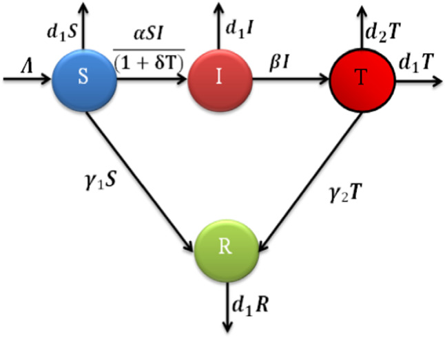
The transfer diagram of proposed discrete COVID-19 model
Rate of change of (S(t)): Susceptible individuals density is increased by new births at the rate , decreased by natural death , and it also decreases via the interaction with infectious individuals. For these, the transmission coefficient is and the parameter is essential to control the susceptible individuals. This population also decreases due to fear and lockdown, which is acquired by the account of the population who are in the secure zone at a constant rate . Consequently, the rate equation for S(t) can be formulated as:
Rate of change of the infected population without treatment (I(t)): The individual who is exposed as infected but not under treatment, and are not infectious for other non-infected individuals. This population increases by interaction with susceptible. The population decreases due to quarantine with the rate (population is in the secure zone at the same rate) and due to the natural death rate () and is expressed by the equation
Rate of change of infected in an isolation ward for treatment not spreading the disease (T(t)): A proportion of infected individuals without treatment transferred to this category after the clinical symptoms of COVID-19 are exposed. These individuals decrease by the rate by getting acquired into the account of the secure zone, the natural death rate, and a death factor caused by COVID-19. The expression for this population is
Rate of change of population is in the secure zone (R(t)): The population increases from susceptible due to fear and lockdown with rate and infected individuals due to in isolation ward for treatment are recovered from the disease at rate A natural death rate condenses these densities; therefore, the expression for this individual is
From the above deliberations, the groups S(t), I(t), T(t) and R(t) denote the densities of the susceptible population (SP), the infected population which spread the disease (IP), infected in an isolated ward for treatment not spreading the disease (TP) and population is in a secure zone (RP), respectively, at time t. Therefore, refers to the total size of the population at the time t. The proposed discrete-time COVID-19 system will discuss for the total human population (N(t)) along with the next initial densities:
| 1 |
Now, using the forward Euler method, we obtain and which are the densities of the populations in discrete-time t. The equations for the generation of the populations can be obtained by replacing t by n, and the proposed discrete-time COVID-19 model is given by:
| 2 |
It is assumed that the total population size is constant, the system of equations can be reduced by one. In particular, the equation for R can be ignored by substituting with in the system. Therefore the proposed discrete-time COVID-19 system can be expressed as follows:
| 3 |
The model parameters are described below:
Equilibrium points and their stability analysis
Existence of equilibrium points
Fixed points of the discrete-time COVID-19 system (3) are obtained via solving the next equations:
We get the following two non-negative equilibrium points:
The disease-free equilibrium (DFE) point , (ii) The endemic equilibrium (EEP) , where , and
Computations of basic reproduction number
The basic reproduction n is one of the most crucial quantity in the analysis of epidemiological models. It enables making effective policies and strategies for control and prevention of diseases. Various approaches for continuous-time models in Castillo-Chavez et al. [6], De Camino-Beck et al. [12], Diekmann et al. [14], Jacquez [22], Thieme [25] and Driessche and Watmough [15] and discrete-time models in Cushing and Ackleh [10], De Camino-Beck and Lewis [11] and Lewis et al. [23] have been presented to obtain suitable analytical expression for .
A well-know technique to estimate is called next-generation matrix method. Let and , where refer to the infected state variables in the model whereas denote the uninfected ones. Suppose that the epidemic model is written as
| 4 |
where is a function. Assume also there is unique DFE point of the model where the Jacobian matrix J has the following form:
| 5 |
The following theorem (Theorem 2.1 in Allen and Driessche [4] and see also De Jong et ali [13]) explains how to compute and demonstrates stability conditions of DFE point.
Theorem 1
Let the system of difference equations (4) possesses single DFE point and the corresponding Jacobian matrix (5) involves non-negative matrices F and H. Furthermore, suppose that is irreducible whereas matrices C and H are achieving , therefore we get Finally, the DFE point of the epidemic model is locally asymptotically stable if and unstable if .
For the our model (3), the J matrix computed at where is given by
The other sub-matrices are extracted as
Now and
Therefore, the next-generation matrix for the proposed discrete-time COVID-19 system (3) is obtained as follows:
As , i.e it is the the spectral radius of the matrix . Then, it can be obtained for the proposed model ( 3)in the form Since all the parameters are positive, the model ( 3) has a unique EEP since It can be shown that DFE point is locally asymptotically stable for and unstable for .
Local stability analysis
The local behavior of the discrete-time pandemic model (3) is presented for each equilibrium point by evaluation of Jacobian matrix at each fixed point of the model. More specifically, the Jacobian Matrix J of the COVID-19 model (3) is given by
where , , , , , , , .
Then, the characteristic equation of J is expressed as where , - , − −
To study the linear stability analysis of non-negative fixed point of the discrete-time system (3), we formulate the next theorem
Theorem 2
Consider the polynomial equation where and are real numbers. Then, the necessary and sufficient conditions that the roots of the equation lie within the open disk are: , , and
Theorem 3
The equilibrium point of the COVID-19 model (3) is locally asymptotically stable at while it is unstable at .
Proof
The matrix of the model (3) can be written as
The three eigenvalues of are , , . Therefore disease-free equilibrium locally asymptotically stable if , i.e. and it is unstable for .
Theorem 4
The fixed point of the proposed map is locally asymptotically stable if , , and
Proof
The matrix for the COVID-19 map (3) is expressed as
Now, the characteristic equation of is , where , , . Therefore, by Jury condition, the fixed point is known to be locally asymptotically stable if , , and
Control strategies of COVID-19 with respect to
This section presents a sensitivity analysis of model parameters to limit COVID-19 cases of India. More specifically, we investigate the most influential parameters in the model on the value of via employing a quantity known as the normalized forward sensitivity indices for the key parameters. The effects of the parameters and are considered in the analysis. The values of estimated parameters given in Table 1 are used long with the initial values , , , , from 21st March 2020 to 16th April 2020. The definition of the normalized forward sensitivity index of f to a parameter is mathematically expressed as:
Table 1.
Explanation of parameters with their real-life value
| Parameters | Meaning | Value | Reference |
|---|---|---|---|
| Recruitment rate of new individuals enter population | 40000 | Estimated | |
| The transmission rate from SP to IP | Estimated | ||
| The transmission rate from IP to TP | 0.05 | Estimated | |
| Parameter measures psychological/inhibitory effect | 0.00042 | Assumed | |
| The transmission rate from SP to RP | 0.0005 | Assumed | |
| The transmission rate from TP to RP | 0.005 | Estimated | |
| Natural death rate of population | 0.00002 | Estimated | |
| Death rate of population caused by COVID-19 | 0.00197 | Estimated |
The sensitivity indices of for the parameters and are given by , , , .
The obtained sensitivity indices indicate that the is positively sensitive to variations in (positively correlated) since . This implies that when is increased by , keeping other parameters constants, will be increased by . For the second parameter, which depicts that if is increased by , then the value of decreases by (negative correlation), provided that the values of other parameters is fixed. For the third parameter , it is found that increasing it by , the value of decreases by , etc. Consequently, when budget limitations is considered in developing countries like India, the planned efforts to suppress and control the spread of COVID-19 is much efficient when focus on tuning suitable values for rather than increasing the numbers of individuals accessing treatment.
Numerical analysis
In this section numerical simulation experiments and comparisons with real data in India are carried out. The following data have been collected from the reports of Ministry of Health and Family Welfare, Government of India in 2020.
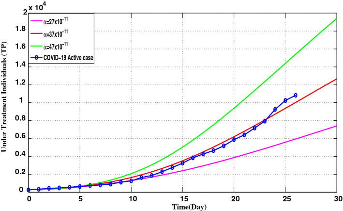
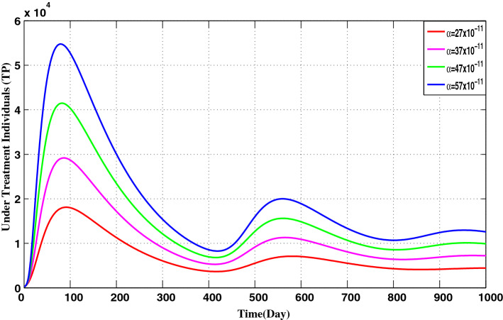
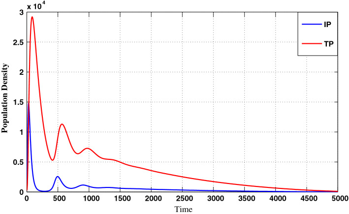
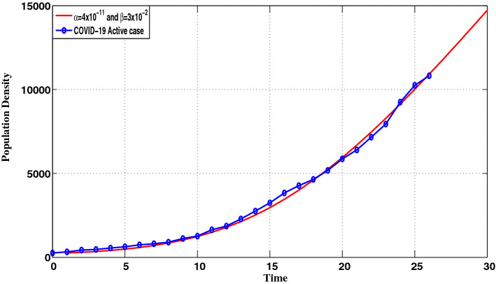
Figures 4, 6, 7 and 8 are obtained according to the parameter given in Table 1 and Table 2. The values of the parameters are set based on the following real data of India. After lockdown in India, the spread of the COVID is recorded as follows (source: ICMR and WHO):
Fig. 4.
Time history of real data of COVID-19 in India and model value of T for different value of
Fig. 6.
Time history of disease for different value of
Fig. 7.
Long time history where disease is vanished
Fig. 8.
Time history of real data of COVID-19 spread in India vs. different values of T
Table 2.
Initial population from real data
| S(0) | I(0) | T(0) |
| 1400 | 256 |
In the proposed model (2), it is known that the most effective parameter in controlling is . Our goal now is to illustrate computationally how effective to spread the disease COVID-19 form humans to the human population. For our support, we have given Table 3 as follows:
Table 4.
Change in different level of
| 0.2614 | 0.5690 | 0.8766 | 1.0149 |
Table 3.
COVID-19 cases in India from 21st March to 16th April
| Date | ||||||||||||||
| Active cases | ||||||||||||||
| Date | ||||||||||||||
| Active cases |
Table 3 represents the value of at different levels of We see that increases if the value of is increasing. That is why is most sensitive with respect to our model. So for a better understanding of the situation, we attain the plot of versus
The is more effective when the value of i.e., the DFE point of system (3) is stable but when the value of then i.e., the DFE point of the model is unstable, and then the situation is more dangerous to our human life. So our aim, in every situation, is to reduce the value of That is why we maintain the policy of lockdown, usage of hand sanitizer, social distancing, mask, etc.
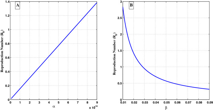
From Fig. 2A, we see that if increases, the value of increases. So it is clear, that if we control the such disease transmission, i.e., , using some precaution such as lockdown, usage of hand sanitizer, social distancing, mask etc. then the disease rate automatically minimise otherwise it should be out of control. That is why is most sensitive with respect to our model. Figure 2B tells that if increases, the value of decreases. These things are matching in our life, which means if the testing rate () of COVID-19 patient increases, the spread of this virus decreases, i.e., For that reason, the Indian Government has taken the initiative in every state to increase the rate of testing as much as possible.
Fig. 2.
The figure shows the variations of with respect to A and B
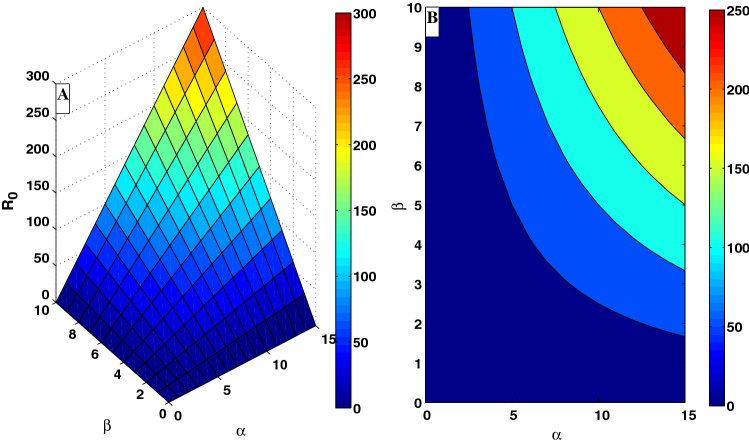
From Fig. 3A, it is demonstrated that when and eventually decreases, the value of decreases too. In Fig. 3B, the contour plots for as a function parameters and are visualized to further explore the effects of the control parameters on values and the dynamics of the proposed model.
Fig. 3.
A The 3D figure shows as a function of and , B The contour plots of the values of with respect to and
The real data regarding COVID-19 pandemic in India are plotted. From Fig. 4, it is noticed that infected patients increase day by day due to the value of disease transmission also increases.
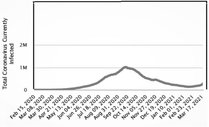
The 27 days of actual epidemic data in India are presented in Fig. 4 as illustration for the critical period of initialization of COVID-19 epidemic spread. After this period, the influences of emergent governmental response and different measures taken out on active cases of coronavirus infections in India are depicted in Fig. 5. The real data presented in Fig. 6 show the evolution of number of COVID-19 infections throughout the first wave of epidemic spread in India (about 367 days). It is observed that, the number of active cases greatly reduced after sufficient long time that is complying with numerical simulation results in Figs. 7 and 8. However, the emergence of mutated versions of coronavirus with highly infection rates causes the subsequent waves of COVID-19 epidemic. This point will be investigated in a separate future work. Figure 6 indicates that if the infection rate increases, the number of infections increases too. The spread of COVID-19 can condense, if the control measures, i.e., social distancing, disease transmission, etc. increases while if they are maintained efficiently, the subsequent outbreaks of COVID-19 can be controlled.
Fig. 5.
Evolution of active cases of COVID-19 infections during the first wave of coronavirus disease in India
Figure 7 shows that after sufficiently long time, the COVID-19 epidemic will vanish. Prevention (i.e., lockdown, social distancing, wash hand regularly, mask) strategies are required to minimize the effect of COVID-19 cases, but it did not diminish the virus. Prevention may be a solution to lessen the outbreak of COVID-19, but the alternate requirement of vaccines and medical treatment is required to avoid the harmfulness of COVID-19 virus worldwide.
Figure 8 shows that the proposed discrete-time pandemic model curve for T is a best-fitted curve for real data of COVID-19 cases in India. For the given data set, it is found that , therefore, there may be a need of strategic action by India on the control policy of COVID-19, which will be able to fight the dangerous situation and prevent the community from COVID-19 in the near future.
Conclusions and observations
This study aims at providing a framework and a guide for addressing the issues of the prevention, early detection, and control of COVID-19 pandemic. Based on the available information by the WHO about COVID-19, including its symptoms, complications, transmission procedure, and how to prevent the transmission, we have proposed and analyzed a compartmental discrete-time COVID-19 epidemic model. The more realistic non-linear incidence rate is employed due to its significance [24, 26, 28]. The basic reproduction number is calculated for the present COVID-19 model both analytically and numerically using the actual database of COVID-19 spread in India. It is demonstrated that for , the proposed model has globally asymptotically stable disease free fixed point.
Regarding the analysis of parameter it is shown that this parameter is a critical parameter in the discrete-time system (2) along with and they play critical role in reducing COVID-19 active cases in India, which may extend the study for any other country. From Fig. 2, it is depicted that when the value of infection transmission rate from SP to IP is less than , the basic reproduction number is less than one and therefore the disease free equilibrium point is asymptotically stable. Similarly, when the value of infection transmission rate from IP to SP is greater than 0.029, the disease free equilibrium point isasymptotically stable and the spread of the disease will die out eventually. The control of these parameters can be achieved via using some precaution such as lockdown, usage of hand sanitizer, social distancing, mask etc. Figure 4 illustrates that real data of COVID-19 spread in India leads to give an approximate value of to parameter while the value of is estimated to be 0.05. This means that a governmental efforts should be directed towards decreasing the value of by appropriate measures
Moreover, from Fig. 6, we see that if the value of disease transmission rate () is increased, the number of infections increases due to the effect of COVID-19 from long term prediction. It is demonstrated that if and are not controlled, then the situation may take the worst form in the future. So far, to reduce the effect of the coronavirus pandemic, the Indian government has taken some meaningful strategies like as reducing the contacts between infected individuals, increasing the effective health care products, maintain the social distancing and washing hands regularly for at least 20 s, etc.
More interestingly, the results also reveal thatCOVID-19 can exhibit oscillatory behavior in future. However, the social distancing measures, efficiency in quarantine, and isolation can control it. Finally, to suppress or minimize the harmful effect of dangerous coronavirus, the most and effective responsibility should be taken by the public of India, and strong cooperation should be rendered to the local administration and Governments. The future work may consider the influences of recent coronavirus mutations such as Delta and Omicron on the dynamics of COVID-19 pandemic. The different cases where the present vaccines can either resist against these virus variants of concern or fail to protect humans against them can be also investigated
Acknowledgements
The authors would like to thank the Editor and anonymous Reviewers for their useful comments and suggestions. The authors would also like to thank the Deanship of Scientific Research, Prince Sattam Bin Abdulaziz University, Al-Kharj, Saudi Arabia, for the support of this work.
Declarations
Conflict of interest
The authors declare that they have no competition of interests.
Ethical approval
This paper does not involve any studies carried out with human participants or on animals.
References
- 1.Ministry of Health and Family Welfare, Government of India 2020. https://www.mohfw.gov.in/. https://www.worldometers.info/coronavirus/country/india/
- 2.Allen LJS. Some discrete-time SI, SIR, and SIS epidemic models. Math. Biosci. 1994;124(1):83–105. doi: 10.1016/0025-5564(94)90025-6. [DOI] [PubMed] [Google Scholar]
- 3.Allen LJS, Burgin AM. Comparison of deterministic and stochastic SIS and SIR models in discrete time. Math. Biosci. 2000;163(1):1–34. doi: 10.1016/S0025-5564(99)00047-4. [DOI] [PubMed] [Google Scholar]
- 4.Allen LJS, Driessche PV. The basic reproduction number in some discrete-time epidemic models. J. Differ. Equ. Appl. 2008;14(10–11):1127–1147. doi: 10.1080/10236190802332308. [DOI] [Google Scholar]
- 5.Biswas MHA, Paiva LT, Pinho MdR. A SEIR model for control of infectious diseases with constraints. Math. Biosci. Eng. 2014;11(4):761–784. doi: 10.3934/mbe.2014.11.761. [DOI] [Google Scholar]
- 6.C. Castillo-Chavez, Z. Feng, W. Huang, On the Computation ofand Its Role on: Mathematical Approaches for Emerging and Reemerging Infectious Diseases: An Introduction (Springer, New York, 2002), pp. 229–250
- 7.Chen T, Rui J, Wang Q, Zhao Z, Cui J, Yin L. A mathematical model for simulating the phase-based transmissibility of a novel coronavirus. Infect. Dis. Poverty. 2020;9(24):1–8. doi: 10.1186/s40249-020-00640-3. [DOI] [PMC free article] [PubMed] [Google Scholar]
- 8.Cheng ZJ, Shan J. 2019 novel coronavirus: where we are and what we know. Infection. 2020;48:1–9. doi: 10.1007/s15010-020-01401-y. [DOI] [PMC free article] [PubMed] [Google Scholar]
- 9.Choi S, Jung E, Choi BY, Hur YJ, Ki M. High reproduction number of Middle East respiratory syndrome coronavirus in nosocomial outbreaks: mathematical modelling in Saudi Arabia and South Korea. J. Hosp. Infect. 2018;99(2):162–168. doi: 10.1016/j.jhin.2017.09.017. [DOI] [PMC free article] [PubMed] [Google Scholar]
- 10.Cushing JM, Ackleh AS. A net reproductive number for periodic matrix models. J. Biol. Dyn. 2012;6(2):166–188. doi: 10.1080/17513758.2010.544410. [DOI] [PubMed] [Google Scholar]
- 11.De Camino-Beck T, Lewis MA. A new method for calculating net reproductive rate from graph reduction with applications to the control of invasive species. Bull. Math. Biol. 2007;69(4):1341–1354. doi: 10.1007/s11538-006-9162-0. [DOI] [PubMed] [Google Scholar]
- 12.De Camino-Beck T, Lewis MA, Driessche PV. A graph-theoretic method for the basic reproduction number in continuous time epidemiological models. J. Math. Biol. 2009;59(4):503–516. doi: 10.1007/s00285-008-0240-9. [DOI] [PubMed] [Google Scholar]
- 13.M.C.M. De Jong, O. Diekmann, J.A.P. Heesterbeek, The computation of for discrete-time epidemic models with dynamic heterogeneity. Math. Biosci. 119(1), 97–114 (1994) [DOI] [PubMed]
- 14.O. Diekmann, J.A.P. Heesterbeek, M.G. Roberts, The construction of nextgeneration matrices for compartmental epidemic models. J. R. Soc. Interface 7(47), 873–885 (2010) [DOI] [PMC free article] [PubMed]
- 15.P.V. Driessche, J. Watmough, Reproduction number and sub-threshold endemic equilibria for compartmental models of disease transmission. Math. Biosci. 180, 29–48 (2002) [DOI] [PubMed]
- 16.A.J. Kucharski, T.W. Russell, C. Diamond, Y. Liu, J. Edmunds, S. Funk, M.E. Rosalind, Early dynamics of transmission and control of COVID-19: a mathematical modelling study. Lancet Infect Dis. (2020). 10.1016/S1473-3099(20)30161-4 [DOI] [PMC free article] [PubMed]
- 17.Gralinski LE, Menachery VD. Return of the coronavirus: 2019-ncov. Viruses. 2020;12(2):135. doi: 10.3390/v12020135. [DOI] [PMC free article] [PubMed] [Google Scholar]
- 18.Heffernan JM, Smith RJ, Wahl LM. Perspectives on the basic reproductive ratio. J. R. Soc. Interface. 2005;2(4):281–293. doi: 10.1098/rsif.2005.0042. [DOI] [PMC free article] [PubMed] [Google Scholar]
- 19.Hernandez-Ceron N, Feng Z, Castillo-Chavez C. Discrete epidemic models with arbitrary stage distributions and applications to disease control. Bull. Math. Biol. 2013;75(10):1716–1746. doi: 10.1007/s11538-013-9866-x. [DOI] [PMC free article] [PubMed] [Google Scholar]
- 20.Huang NE, Qiao F. A data driven time-dependent transmission rate for tracking an epidemic: a case study of 2019-ncov. Sci. Bull. 2020;65(6):425–427. doi: 10.1016/j.scib.2020.02.005. [DOI] [PMC free article] [PubMed] [Google Scholar]
- 21.Huang C, Wang Y, Li X, Ren L, Zhao J, Hu Y, Zhang L, Fan G, Xu J, Gu X, et al. Clinical features of patients infected with 2019 novel coronavirus in Wuhan. china. Lancet. 2020;395(10223):497–506. doi: 10.1016/S0140-6736(20)30183-5. [DOI] [PMC free article] [PubMed] [Google Scholar]
- 22.Jacquez JA, Simon CP, Koopman JS. Core groups and the s for subgroups in heterogeneous SIS and SI models. In: Mollison D , editor. Epidemic Models: Their Structure and Relation to Data. Cambridge: Cambridge University Press; 1995. pp. 279–301. [Google Scholar]
- 23.Lewis MA, Renclawowicz J, Driessche PV, Wonham M. A comparison of continuous and discrete-time West Nile virus models. Bull. Math. Biol. 2006;68(3):491–509. doi: 10.1007/s11538-005-9039-7. [DOI] [PubMed] [Google Scholar]
- 24.Liu W, Levin SA, Iwasa Y. Influence of nonlinear incidence rates upon the behavior of SIRS epidemiological models. J. Math. Biol. 1986;23:187–204. doi: 10.1007/BF00276956. [DOI] [PubMed] [Google Scholar]
- 25.Thieme HR. Spectral bound and reproduction number for infinite-dimensional population structure and time heterogeneity. SIAM J. Appl. Math. 2009;70(1):188–211. doi: 10.1137/080732870. [DOI] [Google Scholar]
- 26.Vargas-De-Leon C, d’Onofrio A. Global stability of infectious disease models with contact rate as a function of prevalence index. Math. Biosci. Eng. 2017;14(4):1–16. doi: 10.3934/mbe.2017053. [DOI] [PubMed] [Google Scholar]
- 27.Wesley CL, Allen LJS, Jonsson CB, Chu YK, Owen RD. A discrete-time rodent-hantavirus model structured by infection and developmental stages. Adv. Stud. Pure Math. 2009;53:387–398. doi: 10.2969/aspm/05310387. [DOI] [Google Scholar]
- 28.Xiao D, Ruan S. Global analysis of an epidemic model with nonmonotone incidence rate. Math. Biosci. 2007;208:419–429. doi: 10.1016/j.mbs.2006.09.025. [DOI] [PMC free article] [PubMed] [Google Scholar]


