Multi-class deep learning segmentation and automated measurements in periodontal sonograms of a porcine model

Abstract

Objectives:

Ultrasound emerges as a complement to cone-beam computed tomography in dentistry, but struggles with artifacts like reverberation and shadowing. This study seeks to help novice users recognize soft tissue, bone, and crown of a dental sonogram, and automate soft tissue height (STH) measurement using deep learning.

Methods:

In this retrospective study, 627 frames from 111 independent cine loops of mandibular and maxillary premolar and incisors collected from our porcine model (N = 8) were labeled by a reader. 274 premolar sonograms, including data augmentation, were used to train a multi class segmentation model. The model was evaluated against several test sets, including premolar of the same breed (n = 74, Yucatan) and premolar of a different breed (n = 120, Sinclair). We further proposed a rule-based algorithm to automate STH measurements using predicted segmentation masks.

Results:

The model reached a Dice similarity coefficient of 90.7±4.39%, 89.4±4.63%, and 83.7±10.5% for soft tissue, bone, and crown segmentation, respectively on the first test set (n = 74), and 90.0±7.16%, 78.6±13.2%, and 62.6±17.7% on the second test set (n = 120). The automated STH measurements have a mean difference (95% confidence interval) of −0.22 mm (−1.4, 0.95), a limit of agreement of 1.2 mm, and a minimum ICC of 0.915 (0.857, 0.948) when compared to expert annotation.

Conclusion:

This work demonstrates the potential use of deep learning in identifying periodontal structures on sonograms and obtaining diagnostic periodontal dimensions.

Introduction

Ultrasound is the most widely used medical imaging modality that combines low cost and portability without ionizing radiation.¹ Recently, the advancement in electronics, including integration and packaging, have enabled ultrasound transducers to have smaller form factors and higher frequencies. Reduced transducer sizes led to new areas of ultrasound application, notably in dentistry. Here, ultrasound has the potential to supplement traditional imaging techniques like two-dimensional (2D) X-ray and 3D cone beam computed tomography (CBCT) currently used by dentists. While excellent for implant surgery planning and hard tissue visualization, CBCT suffers from metal artifacts caused by implants and other metal restorations² and provides limited soft tissue contrast. Ultrasonic imaging, on the other hand, offers high soft tissue contrast. It provides unique cross-sectional views with spatial accuracy of the periodontium,^3–7 peri-implant tissues,⁸ dental caries,⁹ dental pulp spaces¹⁰ and vital intraoral structures.¹¹ These images could bear important value for diagnosing periodontal and peri-implant diseases and evaluate stages of wound healing. However, ultrasound faces limitations of its own, most notably speckle noise and inter operator variability. Speckle noise arises from coherent interference of acoustic waves,¹² which deteriorates image quality with statistical pixel brightness variations. Numerous studies have attempted to address this coherent imaging challenge,^13–17 but speckle remains as an integral part of ultrasound images. Operators incorporate speckles into their diagnosis after months of training and experience.¹⁸ The second problem of inter operator variability stems from the real-time data acquisition nature that ultrasound affords. Although standard planes are defined for many applications of ultrasound,¹⁹ the operator has multiple degrees of rotational freedom that can alter the appearance of anatomical features within the image. To appropriately place the scan plane requires a detailed understanding of the anatomy at hand¹⁸ and familiarity with ultrasound. Together, these two issues make dental sonograms difficult for novices to interpret.

We propose a deep learning (DL)-based segmentation model to address these limitations. The DL model is trained with the appearance and location of critical landmarks (e.g. soft tissue, bone, and crown) by fitting a large number of parameters, such that the model output resembles the annotations provided by an experienced dentist. Once these parameters are optimized, the model can then predict the location of these landmarks within new images. Dentists, guided by this model, should be able to locate these structures more quickly; this may, in turn, reduce interoperator variability and image interpretation time.

Recent work by Nguyen et al. demonstrated the potential of convolutional neural networks (CNN) in segmenting one periodontal structure, i.e., the alveolar bone in ultrasound images.²⁰ Extending from that binary segmentation model, we explored a multi class segmentation network that automatically identifies multiple periodontal and dental structures, including the alveolar bone, gingiva/oral mucosa, and crown in any given image. With these segmentation masks, we propose a rule-based approach to estimate soft tissue height (STH) that has its diagnostic value in assessing the periodontal phenotype.^21,22

Methods and materials

Data acquisition

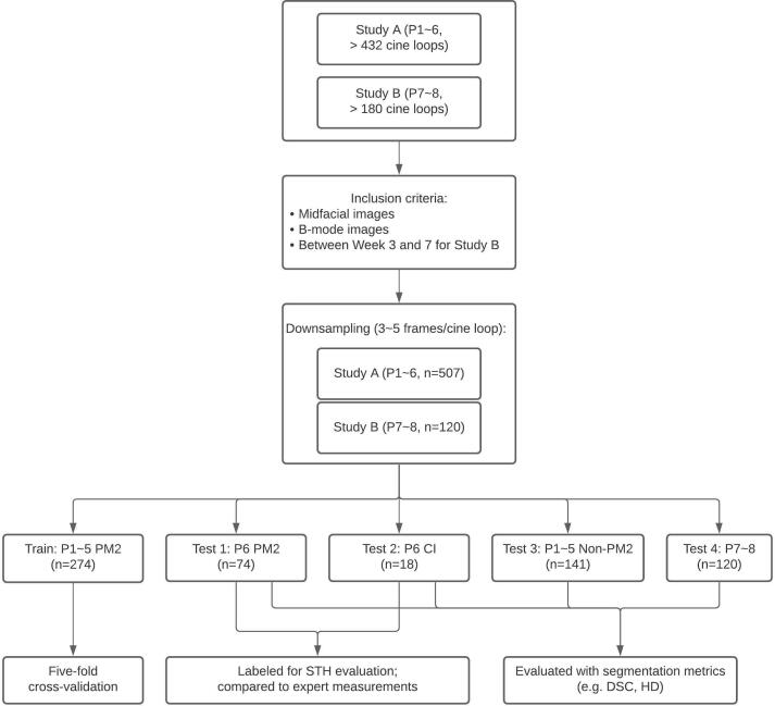
Midfacial B-mode images of a porcine model (N = 6) were used in this retrospective study (Figure 1, Panel A Inset a). These images were part of an accompanying longitudinal study examining ultrasound images of inflamed and healthy periodontal tissues, which was executed under the supervision and with approval from the University of Michigan Institutional Animal Care & Use Committee. The study (Study A in Figure 2) included bilateral maxillary and mandibular second premolars (PM2) of six Yucatan minipigs (P1 ~6) followed for 6 weeks. In the first week, a set of baseline data was taken before ligature was tied around each tooth to promote local bacteria growth and induce inflammation. At each data collection, B-mode images at the midfacial orientation, with 1.5 cm depth of field, were acquired using harmonic imaging (12/24 MHz, clinical ultrasound scanner, ZS-3, Mindray, Mountain View, CA) and a 16.2 × 3 mm 128-element transducer (L25-8, Mindray, Mountain View, CA). A gel pad was affixed to the transducer as a stand-off, to place the tissue region of interest in the elevational focus, i.e., at 7 mm from the probe (Aquaflex® Ultrasound Gel Pad, Parker Laboratories, Inc., Fairfield, NJ). Image bitmaps (720 × 960 pixel) were exported with isotropic spacing of 0.025 mm/pixel. Image cine loops were collected for each tooth, totalling 87 loops across the six pigs at different time points. Three to five frames of each cine loop with minimal image overlap were extracted to form our dataset (Figure 3). Images (n = 159) of the first premolar (PM1), central incisor (CI) and lateral incisor (LI) of P1 ~6 were also acquired but at less regular intervals throughout the study, and were used as a test set to analyze the internal validity of our model in this study. A subset of this is 18 CI sonograms that are all from P6. The results of this small data set are meant to be exploratory and require further testing in the future. Midfacial B-mode images (n = 120) from a more recent, ongoing pig study (Study B in Figure 2) analogous to the original study targets bilateral mandibular and maxillary third and fourth premolar, as well as first molar, with ligature and bacterial induction (P. gingivalis and T. denticola) and a 10-week follow-up. The study comprises images from week three to seven of each tooth of two Sinclair minipigs. Figure 2 outlines the flow of participants.

Figure 1.

Representative photographs and B-mode images. Panel A shows the mandibular right premolars of a sample at baseline; Inset a is the corresponding B-mode image. Panel B and inset b show a photograph and B-mode image of the same tooth one week after ligature is tied around the second mandibular right premolar. Sound waves are transmitted from the right of inset a and b. Panel C shows the transducer at a maxillary right molar. The red arrow denotes the midfacial orientation of the transducer used in this study

Figure 2.

Preclinical study subject flowchart. Study A consisted of six Yucatan minipigs (P1 to P6) and study B consisted of two Sinclair minipigs (P7 and P8). Cineloops typically encompass a time frame of 3–5 s at a frame rate of 19 Hz, and thus contain approximately 60–100 frames, from which 3–5 independent frames are selected. Note that training is performed with premolars of Yucatan (P1–P5) only. Test 1 is performed with (P6) premolars and Test 2 with (P6) central incisors. Test 3 is from the same cohort as training (P1–P5) but different teeth, i.e., non-premolars. Finally, Test 4 is out of breed (Sinclair, as opposed to Yucatan), on both molars and premolars

Figure 3.

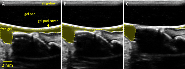
Frames selected from a cine loop of an elastography push. Panel A labels non-clinical structures omitted in Figure 1. The ring-down is an artifact from the acoustic stack within the transducer as well as any impedance mismatch to the lens and attached gel pad. Panels B and C are subsequent frames as the transducer is pressed into the gum. Note that the free gel is pushed away from the sample as a result of the compression

Data labeling and preprocessing

All images were manually labeled by a dentist (E₁) with >23 years of clinical experience and >10 months working with dental ultrasound. Hereinafter, we denote these reference masks with M_E1. We refrain from using the conventional word “ground truth” because all labeling was done on the ultrasound B-mode image without additional inputs (e.g., photographs, histology slides). The labeling was done with the Computer Vision Annotation Tool (CVAT, https://github.com/opencv/cvat). In each image, the soft tissue (including gingiva and muscle), bone, and crown were labeled (Figure 4B). Images were cropped to the actual B-mode image location and resized to fit into GPU memory, resulting in the final size of 320 × 281 and spacing of 0.046 mm/pixel. Each 24-bit image was converted to grayscale by averaging across the RGB channels, demeaned, and normalized by its intensity variance, resulting in an 8-bit grayscale image. B-mode images of P1~5 (n = 274) were used to train and validate three models in a 5-fold cross-validation, and images of P6 (n = 74) were withheld for testing. All training data were augmented with ±10% scaling, ±20% shifting, and horizontal flipping. Additionally, non-premolar images (n = 159) of P1 ~6 and images from P7~8 of a different study (n = 120) were also used to evaluate the robustness of our model.

Figure 4.

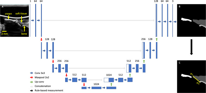
U-Net architecture with input and output images. Panel A shows a typical midfacial sonogram. Panel B shows the segmentation mask provided by the dentist. Panel C shows the definition of STH (yellow) with two endpoints (H₁ and H₂). The rest of the figure is the U-Net architecture chosen in this work

Network description

We chose U-Net for its high segmentation performance in biomedical applications.²³ In brief, the U-Net comprises a contracting and expanding path created with a series of 2 × 2 max-pooling and up-convolution layers, respectively. At each resolution, a series of 3 × 3 convolution layers were used to extract features. In the expanding path, feature maps from the same resolution were directly concatenated with the expanded feature maps to combine low level details with high level context (Figure 4). We randomly initialized all learnable parameters, chose generalized dice loss²⁴ designed for multi class segmentation, and optimized with ADAM.²⁵ To address class imbalance caused by differences in size of each class, the loss in each batch was weighed by the inverse of the area of each class. The number of epochs, batch size, and learning rate were empirically chosen to be 150, 4, and 3 × 10⁻⁵, respectively, based on validation loss of a 5-fold cross-validation. The learning rate was reduced by 90% if validation loss plateaued for five epochs. Training was performed with Pytorch on Google Colaboratory Pro with a Tesla P100 graphics card and the cuDNN library (NVIDIA). In testing, we retained only the largest component in the prediction of each class and compared it to E₁’s annotation. We reported Dice similarity coefficient (DSC), average area intersection (AAI), average area error (AAE), average minimum distance (AMD), and average Hausdorff distance (AHD). In particular, DSC correlates to the ratio of intersection to overlap between M_E1 and M_DL and is calculated with the following:

$${\displaystyle DSC=\frac{2\ast \left|M_{E1\cap M_{DL}}\right|}{\left|M_{E1}\right|+\left|M_{DL}\right|}.}$$

DSC has a range of 0–1 where $DSC=1$ indicates a perfect match between M_E1 and M_DL. AHD is also common in most segmentation literature and defined by

$$\begin{gathered} {\displaystyle AHD=\begin{array}{l}\mathrm{m}\mathrm{a}\mathrm{x}\left\{{\mathrm{m}\mathrm{a}\mathrm{x}}_{x\in M_{E1}}\left\{{\mathrm{m}\mathrm{i}\mathrm{n}}_{y\in M_{DL}}\left\{d(x,y)\right\}\right\}, \\ {\mathrm{m}\mathrm{a}\mathrm{x}}_{y\in M_{DL}}\left\{{\mathrm{m}\mathrm{i}\mathrm{n}}_{x\in M_{E1}}\left\{d(x,y)\right\}\right\}\right\}\end{array}} \end{gathered}$$

AHD is non-negative, and measures the maximum distances between the closest points of two contours. It can be thought of as the worst-case measure between two contours. For all other metrics, please see Supplement for details. Although several area- and distance-based metrics are included in this work, it is worth noting that sonograms of crown and bone simply capture the hyperechoic region proximal to the transducer. In other words, these metrics describe the model’s ability to learn what the reader estimates the boundary to be, as opposed to the true, anatomical crown/bone boundary.

Soft tissue height estimation

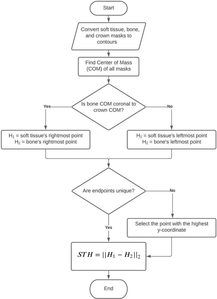
Both E₁ and a second reader with >18 years of experience (E₂) made the STH measurements on a subset of the test set (n = 92; 74 are PM2, and 18 are CI; Test 1 and 2 in Figure 2) without any segmentation masks. E₁ made a second set of measurements 3 months later. We denote the first and second set of measurements made by E₁ with STH_E1a and STH_E1b, respectively. STH_E2 denotes the measurements made by E₂. We define STH as the segment that connects the most coronal point of the soft tissue and the bone crest (Figure 4C). A flow chart (Figure 5) outlines our rule-based algorithm. We report the intraclass correlation (ICC) among STH_E1a, STH_E1b, and STH_E2, and compare them with the output of the rule-based STH algorithm (STHA) applied to M_E1 (STHA_E1) to validate our STH algorithm. Lastly, we compare DL-generated predictions (STHA_DL) with E₁ and E₂’s measurements. Note that STH end points (H₁, H₂) are obtained with a rule-based approach after the DL model segments an image; the end points are not involved in the training of the model in any way. Table 1 lists all abbreviations and their corresponding phrases to aid readers with content comprehension.

Figure 5.

STH estimation algorithm. The algorithm uses an intuitive approach to determine image orientation, by comparing the relative position of bone and crown, with respect to their COMs. Then H₁ and H₂ are assigned to the most coronal soft tissue and bone segmentation mask, respectively. Finally, STH is defined as the Euclidean distance between H₁ and H₂, i.e., their L2 norm, ||$\bullet$||₂. COM, center of mass; STH, soft-tissue height.

Table 1.

List of abbreviations and their corresponding complete phrases

Abbreviation	Complete phrase
Introduction
CBCT	Cone beam computed tomography
DL	Deep learning
Materials and Methods
CI	Central incisors
LI	Lateral incisors
PM1	First premolar
PM2	Second premolar
P1 ~6	Pig one through Pig 6 of the Yucatan breed
P7 ~8	Pig seven through Pig 8 of the Sinclair breed
E1(a,b)	First reader (a,b refers to the first and second replicate)
E2	Second reader
Ma	Mask
STHa	Soft tissue height
STHAa	Rule-based soft tissue height algorithm
Results
DSC	Dice similarity coefficient
AAI	Average area intersection
AAE	Average area error
AHD	Average Hausdorff distance
AMD	Average minimum distance
ICC	Intraclass correlation coefficient
LOA	Limit of agreement

^aSubscript can be added to denote how these measurements are made. For example, STH_E1a refers to the first replicate of STH measurements made by the first reader, and STHA_DL refers to the output of rule-based STH algorithm applied to deep learning prediction masks.

Results

Model performance

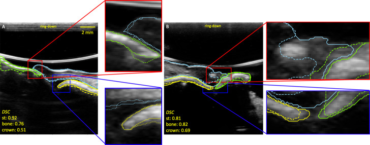
Two sample outputs of the network are shown in Figure 6. The soft tissue segmentation quality was the highest and most consistent across most test sets (Table 2) with respect to area-based metrics including DSC and AAI. Distance-based metrics (e.g. AHD, AMD) suggest a contradictory trend for P6 PM2, but is confounded by the fact that soft tissue has a larger area than bone and crown. Significant reduction in mean crown segmentation quality (e.g. DSC) and increase in uncertainty was observed. The model demonstrated high external validity for soft tissue segmentation but struggled to segment the crown when applied to images of P7 and P8.

Figure 6.

Two examples of reference mask M_E1 (solid lines) and prediction (dashed lines) masks. The sky blue, yellow, and green lines are the soft tissue (st), bone, and crown contours respectively. The DSC show that crown segmentation is poorer than soft tissue and bone. Panel A is a PM2 image of Study A/P6, and Panel B is a PM4 image of Study B/P7. The reader may notice the change in ring-down of the ultrasound system between panel A and B. An ultrasound system update removed most of the ring-down in panel B, which did not affect the segmentation process. DSC, dice similarity coefficient; PM2, premolar 2.

Table 2.

Summary of various segmentation metrics across different test sets

		DSC (%)	AAI (%)	AAE (%)	AMDa (mm)	AHDa (mm)	Average area relative to image size (%)
P6 PM2 (n = 74)	Soft tissue	90.7 ± 4.39	89.6 ± 7.79	9.93 ± 8.16	0.208 ± 0.0719	1.26 ± 0.482	6.38 ± 2.00
	Bone	89.4 ± 4.63	92.3 ± 8.09	14.4 ± 10.7	0.105 ± 0.0307	0.477 ± 0.311	1.77 ± 0.781
	Crown	83.7 ± 10.5	85.8 ± 15.8	24.8 ± 25.5	0.168 ± 0.0943	0.822 ± 0.556	2.01 ± 0.642
P6 CI (n = 18)	Soft tissue	91.1 ± 5.35	88.8 ± 9.08	9.01 ± 7.07	0.239 ± 0.128	1.66 ± 0.833	9.25 ± 1.68
	Bone	86.7 ± 8.27	82.7 ± 13.5	15.6 ± 13.3	0.129 ± 0.0524	0.538 ± 0.363	1.22 ± 0.308
	Crown	43.5 ± 35.8	51.8 ± 42.5	48.5 ± 36.4	1.08 ± 0.931	2.54 ± 1.78	1.42 ± 0.570
P1-5 non PM2 (n = 141)	Soft tissue	92.4 ± 6.67	91.4 ± 6.04	6.47 ± 5.73	0.189 ± 0.0733	1.20 ± 0.504	7.41 ± 2.10
	Bone	79.9 ± 21.0	83.7 ± 23.1	30.2 ± 56.1	0.439 ± 1.27	0.988 ± 1.59	1.13 ± 0.465
	Crown	68.9 ± 20.1	73.3 ± 24.6	47.6 ± 51.1	0.405 ± 0.606	1.89 ± 1.79	1.96 ± 0.801
P7-8 (n = 120)	Soft tissue	90.0 ± 7.16	87.7 ± 10.2	10.9 ± 11.8	0.245 ± 0.142	1.75 ± 0.918	8.18 ± 3.14
	Bone	78.6 ± 13.2	68.2 ± 16.8	29.7 ± 17.3	0.216 ± 0.163	1.12 ± 0.901	1.86 ± 0.682
	Crown	62.6 ± 17.7	48.7 ± 18.4	49.7 ± 19.5	0.408 ± 0.271	1.89 ± 1.28	2.04 ± 0.653

AAE, average area error; AAI, average area intersection; AHD, average Hausdorff distance; AMD, average minimum distance; DSC, dice similarity coefficient.

DSC and AAI are both area-based metrics where 100% is best. AMD and AHD are both distance-based metrics where 0 is best. AAE estimates the extent of under and over segmentation where 0 is best. More detailed definitions of these metrics can be found in the Supplementary Material 1.

^aAHD and AMD values were rounded up to the nearest integer multiple of the image resolution (0.046 mm/pixel) before the mean and standard deviation of the distributions are reported.

STH automation performance

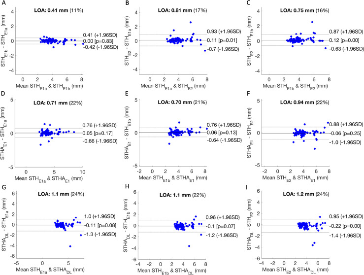
We observed excellent intra operator repeatability with E₁’s STH measurements (ICC = 0.991, 95% Confidence Interval: 0.987, 0.994). The ICC of (STH_E1a, STH_E2) and (STH_E1b, STH_E2) were 0.964 (0.945, 0.977) and 0.968 (0.949, 0.980), respectively. In comparison, the ICC of (STHA_E1, STH_E2) was 0.957 (0.934, 0.971). Comparing STHA_DL to STH_E1a, STH_E1b, and STH_E2, we observed ICC off 0.928 (0.886, 0.950), 0.933 (0.898, 0.956), and 0.915 (0.857, 0.948) respectively. The limit of agreement²⁶ (LOA, 1.96 * standard deviation) in Figure 7 indicates that STHA_E1 agrees more closely with E₁’s STH measurements than E₂’s. Poorer agreement was observed between STHA_DL and either of the experts’ measurements. A statistically significant bias was observed between STHA_DL and E₂.

Figure 7.

Panel A, B, and C compare STH measurements of readers 1 (E₁) and 2 (E₂). Panel D, E, and F compare the output of the deep learning rule-based STH algorithm applied to E₁’s segmentation masks (STHA_E1) to E₁’s measurements (both replicate a and b) and E₂’s. Panel G, H, and I compare the output of STHA applied to the deep learning segmentation masks (STHA_DL) to the same set of expert measurements. LOA (defined as 1.96 × standard deviation) describes the spread of the differences in each comparison. The percentage denotes LOA relative to the average of both methods. LOA, Limit of agreement; STH, soft-tissue height.

Discussion

Generalization and principles

Although our model was trained with a small data set (n = 274 PM2 images, N = 5 pigs), it demonstrated some generalizability when tested against images of different teeth and pigs of a different breed. Specifically, we observed good soft tissue segmentation performance of non-PM2 teeth across the Yucatan minipig breed P1 ~5 and the Sinclair minipig breed P7 ~8 (Table 2). As shown in Figure 6B, and described in the methods, P7 and P8 are a Sinclair breed of pigs using the same imaging system (after a software update).

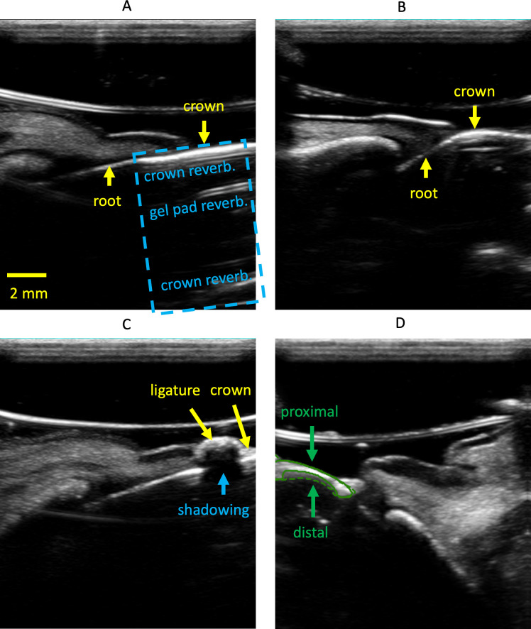
Suboptimal crown segmentation performance was observed across multiple tests, especially when tested on CI sonograms. We attribute the low performance to two factors: (1) In midfacial sonograms of incisors, the crown is collinear with the root and lacks a clear boundary (Figure 8A), leading to inconsistent E₁ annotations. In contrast, the crown and root of premolar images are often at an angle due to furcation, which facilitates more consistent annotation (Figure 8B). (2) The presence of ligatures can increase segmentation difficulty. As described in the methods section, ligature was tied around all teeth to hold down existing (Study A) or introduced (Study B) bacteria and induce inflammation. While ligature was embedded into the coronal gingival tissue of most premolars (Figure 1B), it was most dominant when tied around the incisors. On sonograms, this leads to a strong reflection that is sometimes mistaken for crown, as it can trap air bubbles which result in poor acoustic coupling and a bright reflection. The ligature material itself can act as a strong reflector too (Figure 8C).

Figure 8.

Example artifacts and challenges encountered during this investigation. Panel A shows a midfacial sonogram of an incisor. Crown and root are collinear. The blue dashed box indicates reverberation from the gel pad and within the crown. Panel B shows a midfacial sonogram of a premolar where the crown, neck and root are not collinear. Panel C shows the shadowing effect of a ligature on the crown. Panel D shows the E₁’s annotation (solid line) and prediction (dashed line) masks of the crown. Proximal refers to the side closer to the transducer.

Bone segmentation had poorer generalizability than soft tissue when the model was tested with P7 and P8. We attribute this to the reverberation of signal after the acoustic waves impinge on the hard tissue (Figure 8A). This lack of a clear distal hard tissue boundary, relative to the transducer, led to inconsistent E₁ annotations and poor segmentation (Figure 8D). It is worth noting that the distal boundary of bone and crown are of less interest on ultrasound, as high-frequency sound waves are mostly reflected on impedance boundaries between soft- and hard-tissues. As long as the proximal boundary, relative to the transducer, of the hard tissue can be accurately identified, useful measurements like STH can still be made.

Agreement with established research

To the authors’ best knowledge, this study is among the first to explore the feasibility of deep learning in interpreting ultrasound periodontal images. The proposed model achieves an average DSC of 86.7% for bone segmentation in CI images, and is comparable to the 85.3% reported by Nguyen et al who exclusively investigated CI images. While our reported AHD for the alveolar bone of CI images (0.538 ± 0.363 mm) is worse than Nguyen et al’s (0.32 ± 0.19 mm), our model is specifically trained with PM2 images. We expect a lower HD if the model were trained with CI images. However, we did not perform this test as most of our images are non-CI.

Extending beyond the alveolar bone crest that Nguyen et al identified, our work included the automated measurement of STH. STH is considered an integral part of periodontal phenotype parameters, comprising the gingival sulcus, connective tissue attachment and epithelial attachment under histology. Variability in STH dimension has been found and has important clinical implications, e.g. periodontal-restorative interface determination and the risk of gingival recession.²⁷ Currently, the invasive bone sounding method of placing a periodontal probe with a 1 mm measurement resolution in the sulcus until it reaches bone under local anesthesia is used to measure STH. Our post-processing, rule-based algorithm had a limit of agreement (LOA) of <0.94 mm across several sets of expert measurements (Figure 7F), which compares favorably against the LOA between E₁ and E₂ of 0.75 mm (Figure 7C). Our predicted STH (STHA_DL) has a larger LOA of 1.2 mm (Figure 7I), but it may improve if we train a model with images without ligature. With more validation, we believe that ultrasound could be a useful tool for estimating STH non-invasively and accurately for research and clinical care.

A more sophisticated definition of STH

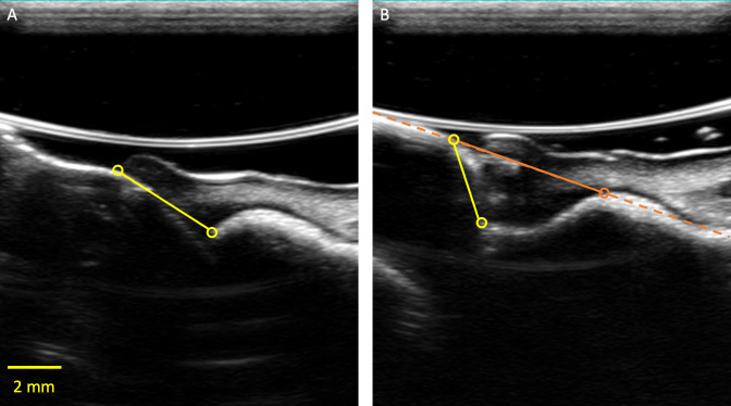
As defined earlier, the STH in this work is the segment that connects the most coronal points of the bone and soft tissue. Although this approach produced an accurate estimate of the dentists’ measurements in most cases (Figure 9A), both E₁ and E₂ were less certain about the optimal STH definition in 10% of the test images, where the bone extends further towards the crown, making the STH nearly vertical (Figure 9B). In such images, a more sophisticated definition of STH might be appropriate. One approach is to find the best fit line through the crown and the bone, and use random sample consensus (RANSAC) to eliminate any significant outliers. However, having multiple STH algorithms would require a separate classification algorithm to identify which to use for a given image.

Figure 9.

Panel A presents a case where both E₁ and E₂ could confidently identify STH (made by E₁ in this image). Panel B presents a case where the yellow points that E₁ annotated could be ambiguous. An alternative STH definition that involves identifying the best fit line (orange dash) through the bone and crown, and identifying the first intersection between the line and the bone (orange circle) should be explored in a future study. STH, soft-tissue height

Limitations

There are several limitations with this study. First, the data set was relatively small and may also not be generalizable to humans. Second, there was only one reference reader who labeled all training, validation, and testing images in model creation. Future studies will focus on acquiring a larger, more diverse (race, age, and pathologies) human data set with reference labels from multiple readers. Independently, the robustness of our rule-based approach for STH measurement should also be examined against manual probing, incorporating a more complex algorithm if necessary.

Conclusion

In this study, we proposed a deep learning algorithm to segment soft tissue, bone, and crown of a dental sonogram. We demonstrated the effectiveness of our approach and the accuracy of the automated STH derived with a rule-based algorithm. The work provides preliminary support for incorporating deep learning to accelerate the clinical adoption of dental ultrasound based periodontal quantification. Algorithmic stability with respect to tooth type as well as breed, may indicate stability for human to human variation as well as normal to anatomical pathology variation. Lastly, real-time implementation of this algorithm on a clinical ultrasound scanner is potentially feasible and could bring this technology closer to clinical use.

REFERENCES

- 1.Klibanov AL, Hossack JA. Ultrasound in radiology: from anatomic, functional, molecular imaging to drug delivery and image-guided therapy. Invest Radiol 2015; 50: 657–70. [DOI] [PMC free article] [PubMed] [Google Scholar]
- 2.Vanderstuyft T, Tarce M, Sanaan B, Jacobs R, de Faria Vasconcelos K, Quirynen M. Inaccuracy of buccal bone thickness estimation on cone-beam CT due to implant blooming: an ex-vivo study. J Clin Periodontol 2019; 46: 1134–43. doi: 10.1111/jcpe.13183 [DOI] [PubMed] [Google Scholar]
- 3.Chan H-L, Wang H-L, Fowlkes JB, Giannobile WV, Kripfgans OD. Non-ionizing real-time ultrasonography in implant and oral surgery: a feasibility study. Clin Oral Implants Res 2017; 28: 341–7. doi: 10.1111/clr.12805 [DOI] [PubMed] [Google Scholar]
- 4.Chan H-L, Sinjab K, Li J, Chen Z, Wang H-L, Kripfgans OD. Ultrasonography for noninvasive and real-time evaluation of peri-implant tissue dimensions. J Clin Periodontol 2018; 45: 986–95. doi: 10.1111/jcpe.12918 [DOI] [PubMed] [Google Scholar]
- 5.Tattan M, Sinjab K, Lee E, Arnett M, Oh T-J, Wang H-L, et al. Ultrasonography for chairside evaluation of periodontal structures: a pilot study. J Periodontol 2020; 91: 890–9. doi: 10.1002/JPER.19-0342 [DOI] [PubMed] [Google Scholar]
- 6.Tsiolis FI, Needleman IG, Griffiths GS. Periodontal ultrasonography. J Clin Periodontol 2003; 30: 849–54. doi: 10.1034/j.1600-051X.2003.00380.x [DOI] [PubMed] [Google Scholar]
- 7.Chifor R, Hedeşiu M, Bolfa P, Catoi C, Crişan M, Serbănescu A. The evaluation of 20 MHz ultrasonography, computed tomography scans as compared to direct microscopy for periodontal system assessment. Med Ultrason 2011; 13: 120–6. [PubMed] [Google Scholar]
- 8.Chan H-L, Kripfgans OD. Ultrasonography for diagnosis of peri-implant diseases and conditions: a detailed scanning protocol and case demonstration. Dentomaxillofac Radiol 2020; 49: 20190445. doi: 10.1259/dmfr.20190445 [DOI] [PMC free article] [PubMed] [Google Scholar]
- 9.Kim J, Shin TJ, Kong HJ, Hwang JY, Hyun HK. High-Frequency ultrasound imaging for examination of early dental caries. J Dent Res 2019; 98: 363–7. doi: 10.1177/0022034518811642 [DOI] [PubMed] [Google Scholar]
- 10.Szopinski KT, Regulski P. Visibility of dental pulp spaces in dental ultrasound. Dentomaxillofac Radiol 2014; 43: 20130289. doi: 10.1259/dmfr.20130289 [DOI] [PMC free article] [PubMed] [Google Scholar]
- 11.Barootchi S, Chan H-L, Namazi SS, Wang H-L, Kripfgans OD. Ultrasonographic characterization of lingual structures pertinent to oral, periodontal, and implant surgery. Clin Oral Implants Res 2020; 31: 352–9. doi: 10.1111/clr.13573 [DOI] [PMC free article] [PubMed] [Google Scholar]
- 12.Burckhardt CB. Speckle in ultrasound B-mode scans. IEEE Transactions on Sonics and Ultrasonics 1978; 25: 1–6. doi: 10.1109/T-SU.1978.30978 [DOI] [Google Scholar]
- 13.Traney G, Allison JW, Smith SW, von Ramm OT. A quantitative approach to speckle reduction via frequency compounding. Ultrason Imaging 1986; 8: 151–64. doi: 10.1016/0161-7346(86)90006-4 [DOI] [PubMed] [Google Scholar]
- 14.Rohling R, Gee A, Berman L. Three-dimensional spatial compounding of ultrasound images. Med Image Anal 1997; 1: 177–93. doi: 10.1016/S1361-8415(97)85009-8 [DOI] [PubMed] [Google Scholar]
- 15.Jespersen SK, Wilhjelm JE, Sillesen H. Multi-angle compound imaging. Ultrason Imaging 1998; ; 20: 81–102Apr 1. doi: 10.1177/016173469802000201 [DOI] [PubMed] [Google Scholar]
- 16.Coupe P, Hellier P, Kervrann C, Barillot C. Nonlocal means-based speckle filtering for ultrasound images. IEEE Transactions on Image Processing 2009; 18: 2221–9. doi: 10.1109/TIP.2009.2024064 [DOI] [PMC free article] [PubMed] [Google Scholar]
- 17.Mateo JL, Fernández-Caballero A. Finding out general tendencies in speckle noise reduction in ultrasound images. Expert Syst Appl 2009; 36: 7786–97. doi: 10.1016/j.eswa.2008.11.029 [DOI] [Google Scholar]
- 18.Naredo E, Bijlsma JWJ. Becoming a musculoskeletal ultrasonographer. Best Pract Res Clin Rheumatol 2009; 23: 257–67. doi: 10.1016/j.berh.2008.12.008 [DOI] [PubMed] [Google Scholar]
- 19.Dudley NJ, Chapman E. The importance of quality management in fetal measurement. Ultrasound Obstet Gynecol 2002; 19: 190–6. doi: 10.1046/j.0960-7692.2001.00549.x [DOI] [PubMed] [Google Scholar]
- 20.Nguyen KCT, Duong DQ, Almeida FT, Major PW, Kaipatur NR, Pham TT, et al. Alveolar bone segmentation in intraoral Ultrasonographs with machine learning. J Dent Res 2020; 99: 1054–61. doi: 10.1177/0022034520920593 [DOI] [PubMed] [Google Scholar]
- 21.Chambrone L, Avila-Ortiz G. An evidence-based system for the classification and clinical management of non-proximal gingival recession defects. J Periodontol 2021; 92: 327–35. doi: 10.1002/JPER.20-0149 [DOI] [PubMed] [Google Scholar]
- 22.Tavelli L, Barootchi S, Avila-Ortiz G, Urban IA, Giannobile WV, Wang H-L. Peri-Implant soft tissue phenotype modification and its impact on peri-implant health: a systematic review and network meta-analysis. J Periodontol 2021; 92: 21–44. doi: 10.1002/JPER.19-0716 [DOI] [PubMed] [Google Scholar]
- 23.Ronneberger O, Fischer P, Brox T. U-Net: Convolutional Networks for Biomedical Image Segmentation. In: Navab N, Hornegger J, Wells W. M, Frangi A. F, eds.Medical Image Computing and Computer-Assisted Intervention – MICCAI 2015. Cham: Springer International Publishing; 2015. pp. 234–41. [Google Scholar]
- 24.Sudre CH, Li W, Vercauteren T, Ourselin S, Jorge Cardoso M. Generalised dice overlap as a deep learning loss function for highly unbalanced segmentations. Lecture Notes in Computer Science 2017;: 240–8. [DOI] [PMC free article] [PubMed] [Google Scholar]
- 25.Kingma DP, Ba J. Adam: a method for stochastic optimization. 2017. Available from: http://arxiv.org/abs/1412.6980.
- 26.Martin Bland J, Altman D. Statistical methods for assessing agreement between two methods of clinical measurement. The Lancet 1986; 327: 307–10. doi: 10.1016/S0140-6736(86)90837-8 [DOI] [PubMed] [Google Scholar]
- 27.Kois JC. The restorative-periodontal interface: biological parameters. Periodontol 2000 1996; 11: 29–38. doi: 10.1111/j.1600-0757.1996.tb00180.x [DOI] [PubMed] [Google Scholar]
Associated Data
This section collects any data citations, data availability statements, or supplementary materials included in this article.