Cross-Axis projection error in optically pumped magnetometers and its implication for magnetoencephalography systems

Abstract

Optically pumped magnetometers (OPMs) developed for magnetoencephalography (MEG) typically operate in the spin-exchange-relaxation-free (SERF) regime and measure a magnetic field component perpendicular to the propagation axis of the optical-pumping photons. The most common type of OPM for MEG employs alkali atoms, e.g. ⁸⁷ Rb, as the sensing element and one or more lasers for preparation and interrogation of the magnetically sensitive states of the alkali atoms ensemble. The sensitivity of the OPM can be greatly enhanced by operating it in the SERF regime, where the alkali atoms’ spin exchange rate is much faster than the Larmor precession frequency. The SERF regime accommodates remnant static magnetic fields up to ±5 nT. However, in the presented work, through simulation and experiment, we demonstrate that multi-axis magnetic signals in the presence of small remnant static magnetic fields, not violating the SERF criteria, can introduce significant error terms in OPM’s output signal. We call these deterministic errors cross-axis projection errors (CAPE), where magnetic field components of the MEG signal perpendicular to the nominal sensing axis contribute to the OPM signal giving rise to substantial amplitude and phase errors. Furthermore, through simulation, we have discovered that CAPE can degrade localization and calibration accuracy of OPM-based magnetoencephalography (OPM-MEG) systems.

1. Introduction

Magnetoencephalography (MEG) is a non-invasive method for measuring magnetic fields emanating from the brain’s neural activity (Hämäläinen et al., 1993). The two main sensors for measuring sub-pT magnetic fields are superconducting quantum interference devices (SQUIDs) (Zimmerman et al., 1970) and optically pumped magnetometers (OPMs) (Xia et al., 2006; Johnson et al., 2010). Historically, SQUIDs have been the sensor of choice for MEG; however, there has been a steady increase in the use of OPM sensors for MEG over the last decade (Cohen-Tannoudji et al., 1970; Boto et al., 2018; Borna et al., 2020; Iivanainen et al., 2020; Nardelli et al., 2020). Unlike SQUIDs, OPMs operate above room temperature (∼150 °C for alkali-atom-based OPMs) and hence do not require the SQUID’s thick dewar, which provides insulation between liquid helium and the subject’s head. As a result, OPMs can be used in ambulatory scenarios, have lower initial/maintenance costs, and benefit from enhanced signal-to-noise ratio (SNR). The smaller sensor standoff (sensor-to-source distance) of the OPM sensors improves the signal strength as the magnetic field’s magnitude drops inversely with the square of the source-sensor distance (Boto et al., 2016; Iivanainen et al., 2017). The OPM’s improved SNR is a driving factor in its rising popularity for MEG applications as, in theory, it leads to better spatial-resolution for source-localization.

To benefit from the OPM’s enhanced SNR, measurement errors should be minimized. A SQUID measures the magnetic flux through its pick-up coil; hence, the SQUID’s sensing axis and center are precisely defined by the coil’s coordinates and geometry. Furthermore, there are no ambient field-dependent errors in the SQUID’s output signal. OPM sensors on the other hand do not have a precisely defined coordinate-based sensing axis or center, and they have inherent errors for cross-axis fields (Cohen-Tannoudji et al., 1970; Seltzer and Romalis 2004) if not carefully controlled. Previously, systematic gain error in the presence of low frequency drift has been derived analytically for OPMs (Boto et al., 2018; Iivanainen et al., 2019). In this paper, through simulation and experiment, we examine the OPM’s systematic error with multi-axis magnetic signals in the presence of remnant static magnetic fields; such conditions give rise to an error large enough to diminish the OPM’s enhanced SNR and degrade source localization capabilities of the OPM-MEG systems. We experimentally induced the cross-axis projection error (CAPE) in our OPM sensors and successfully simulated the erroneous signals. Furthermore, we simulated the impact of the OPMs’ CAPE on the localization capability of our OPM-MEG system under realistic conditions. This paper is organized as follows: In Sec. II, we discuss the theory of optically pumped magnetometers and formulate the inherent CAPE terms. Sec. III describes the experimental setup and compares the simulation results to that of the experiment. And finally, section IV concludes the paper.

2. Theory

In OPMs, also termed atomic magnetometers, the atomic spins evolve as a function of external magnetic field, and by measurement of the atomic spins one can infer the external magnetic field. By working through the quantum mechanics of the Hamiltonian describing coupling of the spin of the unpaired electron in an alkali atom to an external magnetic field, one can arrive at the evolution of atomic spins as approximated by a Bloch equation (Seltzer 2008):

$$\{\begin{array}{l}\frac{d\mathbf{\text{P}}}{dt}=\frac{1}{q}\left[\gamma \mathbf{\text{P}}\times \mathbf{\text{B}}+R_{O\mathbf{P}}\left(\mathbf{\text{s}}-\mathbf{\text{P}}\right)-R_{rel}\mathbf{\text{P}}\right]\hfill \\ R_{rel}=\frac{1}{T_2}+{\mathrm{\Gamma }}_{PR}\hfill \end{array}$$ (1)

In this equation, diffusion is ignored; P is the electron spin polarization vector of the atom varying between −1 and 1; B is the magnetic field vector; γ is the gyromagnetic ratio of the orbital electron; q is the nuclear slowing down factor of the ⁸⁷ Rb; R_OP is the optical pumping rate of the pumping laser beam; s is the spin of the optical pumping with a magnitude of unity when the pump laser is circular polarized; R_rel is the relaxation rate from spin destruction, diffusion to the cell walls, spin exchange, and probe beam depolarization rates (Γ_PR). The nuclear slowing down factor q = q(B, P) is in general a function of P and B and is an averaged parameter related to atoms being in the spin-exchange-relaxation-free (SERF) regime (Savukov and Romalis 2005); in this regime the alkali atoms’ spin exchange rate $\left(T_{se}^{\hspace{0.17em}\hspace{0.17em}-1}\right)$ is much faster than Larmor precession frequency, obeying the inequality γBT_se ≪ 1; where B is the magnitude of the total magnetic field including a potential remnant static magnetic field. Hence, this regime accommodates remnant static magnetic fields obeying the aforementioned inequality.

The output of the OPM sensor reflects the component of the electron spin polarization (P) along the path of the probe laser beam. The probe laser beam can be the same as the pumping laser beam (Knappe et al., 2012; Shah and Wakai 2013) where transmitted pump power carries the polarization information; it can also be, as it is in our case, a second linearly-polarized beam detuned from the D₂ transition of the alkali atoms (Colombo et al., 2016), where the magnetic field is encoded in the laser’s polarization through Faraday rotation. However, regardless of the probing scheme, the OPM’s output reflects the component of the electron spin polarization along the probe propagation axis. Hence, we will focus on the behavior of the spin polarization for the rest of the presented analysis. Note that we are restricting our analysis to where the probe beam is parallel to the pump beam, but there are other possible probing schemes (Kominis et al., 2003).

In this analysis we assume that the external magnetic field to be sensed is on the x-axis and the pump/probe laser propagation is along the z-axis $\left(\mathbf{\text{s}}=\widehat{z}\right)$ as shown in Fig. 1. Furthermore, we extract the OPM’s output from the atoms’ polarization component aligned with the pumping laser propagating along the z-axis. There is no general closed-form solution for the Bloch equations; however, (Cohen-Tannoudji et al., 1970) derives a closed-form formula for a special case as explained below. If the magnetic signal to be sensed is on the x-axis, due to cross product of the Bloch equations (1), the atomic polarization will have components on the y- and z-axis, and to reduce the number of equations, we can define P_± = P_z ± iP_y. Regrouping the Bloch equations gives the following:

$$\{\begin{array}{l}\frac{d{P}_{\pm }}{dt}=\left(\pm i\frac{\gamma }{q}{B}_x-\frac{{\text{R}}_{rel+}{R}_{OP}}{q}\right)p_{\pm }+\frac{R_{OP}}{q}+\left(\frac{\gamma }{q}{B}_q\mp i\frac{\gamma }{q}{B}_z\right)P_x\hfill \\ \frac{d{P}_x}{dt}=\left(-\frac{{\text{R}}_{rel}+R_{OP}}{q}\right)P_x+\left(\frac{\gamma }{q}{B}_z\right)P_y-\left(\frac{\gamma }{q}{B}_y\right)P_z\hspace{0.17em}\hspace{0.17em}\hspace{0.17em}\hspace{0.17em}\hspace{0.17em}\hspace{0.17em}\hspace{0.17em}\hspace{0.17em}\hspace{0.17em}\hspace{0.17em}\hspace{0.17em}\hspace{0.17em}\hspace{0.17em}\text{(2b)}\hfill \end{array}$$ (2a)

Fig. 1.

The OPM sensor’s coordinates. Circularly (linearly)-polarized pump (probe)-beam are coaligned on the z-axis; the external magnetic field vector is out of the plane opposite the x-axis.

If the magnetic field on the y- and z-axis is such that the induced Larmor precession frequency (γB_z, γB_y) is much smaller than the relaxation rate (R_rel+ R_OP), Eq. (2)a yields a zero steady state polarization in the x-axis (P_x); hence, the two equations can be decoupled and Eq. (2)a can be solved in closed-form. It is instructive to write the total field in time-domain as B₀ + B_scos(ω_st) + B_mcos(ω_mt), where B₀ = (B_x0, B_y0, B_z0) is a static remnant field, B_s = (B_xs, B_ys, B_zs) is the signal field amplitude, and B_m = (B_xm, B_ym, B_zm) is the modulating field amplitude. In this analysis, B_m has only components along the x-axis, i.e. B_ym = B_zm = 0. The sensitive axis is modulated/dithered using a sinusoid $\left(\widehat{B_{xm}}\left(t\right)=B_m\cos \left({\omega }_{m}t\right)\right)$ with an amplitude of B_m at an angular frequency (ω_m) much larger than the Larmor precession frequency due to B₀ and B_s. The sensitive axis also contains the magnetic signal to be sensed $\left(\widehat{B_{xs}}\left(t\right)=B_{xs}\cos \left({\omega }_{s}t\right)\right)$. Modulating the sensitive axis up-converts the signal of interest $\left(\widehat{B_{xs}}\left(t\right)\right)$ to the modulation frequency (ω_m). Making the substitution τ = 1∕(R_rel+R_OP), the obtained response of the OPM at the modulation frequency takes the form of a dispersion curve with a width of 2∕(γτ) (Cohen-Tannoudji et al., 1970):

$$P_z={\text{R}}_{op}\tau \hspace{0.17em}{J}_0\left(\frac{\gamma B_m}{q{\omega }_m}\right)J_1\left(\frac{\gamma B_m}{q{\omega }_m}\right)\frac{\gamma \tau \widehat{B_{xs}}\left(t\right)}{1+{\left(\gamma \tau \widehat{B_{xs}}\left(t\right)\right)}^2}\sin \left({\omega }_{m}t\right)$$ (3)

J_n the n^th order Bessel functions of the first kind. $\widehat{B_{xs}}\left(t\right)$ is assumed to be quasistatic, where its frequency components are much less than l/τ. As can be seen, the information about the external magnetic field of interest is embedded in the amplitude of P_z at the modulation frequency and can be extracted using lock-in detection (Scofield, 1994). Other than linearizing the response about zero field, another advantage of lock-in detection is alleviating the flicker noise arising from low-frequency laser noise and temperature drift in the vapor cell.

If the aforementioned assumptions that allowed a closed-form solution for Bloch equations are violated, Eq. (3) is no longer an accurate representation of the OPM’s output, and the fidelity of the sensed magnetic field $\left(\widehat{B_{xs}}\left(t\right)\right)$ will be compromised. Specifically, in the presence of a large static magnetic field on the laser’s propagation axis, i.e. the z-axis, such that Larmor precession frequency (γB_z) is no longer negligible compared to total relaxation rate (1∕τ), a cross-axis projection term can constitute a significant portion of the electron spin polarization or OPM’s output signal.

With non-negligible static magnetic field along the laser’s propagation axis (B_z), if we assume $\gamma B_y\ll \gamma B_x$, the Bloch equations’ system of ordinary differential Eq. (1), decouples and simplifies to a third order ordinary differential equation for P_z:

$$\begin{array}{l}\frac{d^3{P}_z}{d^{3}t}\left({\omega }_x^{\hspace{0.17em}\hspace{0.17em}2}\right)+\frac{d^2{P}_z}{d^{2}t}\left(3\mathrm{\Gamma }{\omega }_x^{\hspace{0.17em}\hspace{0.17em}2}-2{\omega }_x\frac{d{\omega }_x}{dt}\right)\\ \hspace{0.17em}\hspace{0.17em}\hspace{0.17em}\hspace{0.17em}+\frac{d{P}_z}{dt}\left({\omega }_x^{\hspace{0.17em}\hspace{0.17em}4}+{\omega }_z^{\hspace{0.17em}\hspace{0.17em}2}{\omega }_x^{\hspace{0.17em}\hspace{0.17em}2}+3{\mathrm{\Gamma }}^2{\omega }_x^{\hspace{0.17em}\hspace{0.17em}2}-4\mathrm{\Gamma }{\omega }_x\frac{d{\omega }_x}{dt}-{\omega }_x\frac{d^2{\omega }_x}{d^{2}t}+2{\left(\frac{d{\omega }_x}{dt}\right)}^2\right)\\ \hspace{0.17em}\hspace{0.17em}\hspace{0.17em}\hspace{0.17em}+P_z({\omega }_z{\omega }_x^{\hspace{0.17em}\hspace{0.17em}3}{\omega }_y+{\omega }_x^{\hspace{0.17em}\hspace{0.17em}3}\frac{d{\omega }_x}{dt}-2{\mathrm{\Gamma }}^2{\omega }_x\frac{d{\omega }_x}{dt}+\mathrm{\Gamma }{\omega }_z^{\hspace{0.17em}\hspace{0.17em}2}{\omega }_x^{\hspace{0.17em}\hspace{0.17em}2}-\mathrm{\Gamma }{\omega }_x\frac{d^2{\omega }_x}{d^{2}t}\\ \hspace{0.17em}\hspace{0.17em}\hspace{0.17em}\hspace{0.17em}\hspace{0.17em}\hspace{0.17em}\hspace{0.17em}\hspace{0.17em}\hspace{0.17em}\hspace{0.17em}\hspace{0.17em}\hspace{0.17em}\hspace{0.17em}\hspace{0.17em}\hspace{0.17em}\hspace{0.17em}+2\mathrm{\Gamma }{\left(\frac{d{\omega }_x}{dt}\right)}^2+\mathrm{\Gamma }{\omega }_x^{\hspace{0.17em}\hspace{0.17em}4}+{\mathrm{\Gamma }}^3{\omega }_x^{\hspace{0.17em}\hspace{0.17em}2})\\ \hspace{0.17em}\hspace{0.17em}\hspace{0.17em}\hspace{0.17em}+\frac{{\text{R}}_{OP}}{q}\left({\omega }_x\frac{d^2{\omega }_x}{d^{2}t}+2\mathrm{\Gamma }{\omega }_x\frac{d{\omega }_x}{dt}-2{\left(\frac{d{\omega }_x}{dt}\right)}^2-{\mathrm{\Gamma }}^2{\omega }_x^{\hspace{0.17em}\hspace{0.17em}2}-{\omega }_z^{\hspace{0.17em}\hspace{0.17em}2}{\omega }_x^{\hspace{0.17em}\hspace{0.17em}2}\right)=0\end{array}$$ (4)

where $\text{ω}=\frac{\mathbf{\gamma }}{q}\mathbf{\text{B}}$, and $\mathrm{\Gamma }=\frac{{\text{R}}_{rel}}{q}$. Solving this equation yields the electron spin polarization along the laser’s propagation axis (P_z); numerical simulation of Eq. (4) yields very similar results to that of the complete Bloch equations, however solving it in closed form is not possible. Investigating this equation can give us insight into the CAPE; two terms containing the cross-axis leakage are ${\omega }_z{\omega }_x^{\hspace{0.17em}\hspace{0.17em}3}{\omega }_y$ and ${\omega }_z^{\hspace{0.17em}\hspace{0.17em}2}{\omega }_x^{\hspace{0.17em}\hspace{0.17em}2}$; hence, the deterministic error is present if a multi-axis signal is accompanied by a static magnetic field $\left({\omega }_z=\frac{\gamma }{q}{B}_{z0}\right)$ along the laser’s propagation axis. Numerical simulation of Eq. (4) reveals that the cross-axis term $\left({\omega }_z^{\hspace{0.17em}\hspace{0.17em}2}{\omega }_x^{\hspace{0.17em}\hspace{0.17em}2}\right)$ only impacts the gain but not the phase, whereas the term ${\omega }_z{\omega }_x^{\hspace{0.17em}\hspace{0.17em}3}{\omega }_y$ induces gain and phase errors. In this context, phase error is the phase difference between the sensor’s output and the coil driver (reference) signal; amplitude error is the deviation of the OPM’s output from that of the ideal case with no cross-axis leakage present.

For a modulated OPM sensor, the output is extracted using lock-in detection and ideally is a linear function of the magnetic field along the sensitive axis (excluding the modulating field):

$$P_z=f\left(B_x,B_y,B_z\right)\approx G_{OPM}Re\left\{\widehat{B_{xs}}\left(t\right)e^{i\left({\theta }_{OPM}+{\theta }_{CAPE}\right)}\right\}+O_{CAPE}$$ (5)

In Eq. (5), for an ideal OPM sensor, the CAPE term O_CAPE and phase shift θ_CAPE are zero. Furthermore, G_OPM and θ_OPM are independent of the magnetic fields on all the axes and are only a function of the system’s high-level parameters; this in fact is the case for Eq. (3), where there is no phase error (θ_CAPE = 0), and the quasistatic gain is given by:

$$G_{OPM}\approx {\text{R}}_{op}\tau J_0\left(\frac{\gamma B_m}{q{\omega }_m}\right)J_1\left(\frac{\gamma B_m}{q{\omega }_m}\right)\gamma \tau$$ (6)

However, Eq. (4) reveals that by considering the cross-axis leakage, the system’s response can be a function of magnetic signals on all axes. Hence, other than high level system parameters, both O_CAPE and θ_CAPE are functions of all magnetic field components, i.e. O_CAPE = (B_x, B_y, B_z) and θ_CAPE = g(B_x, B_y, B_z). Hence, there is an inherent error term in the OPM’s output manifested as amplitude (O_CAPE) and phase (θ_CAPE) error. It is possible to derive a closed-form formula for the OPM signal for quasistatic fields (Cohen-Tannoudji et al., 1970):

$$\begin{gathered} P_z\approx {\text{R}}_{op}\tau J_0\left(\frac{\gamma B_m}{q{\omega }_m}\right)J_1\left(\frac{\gamma B_m}{q{\omega }_m}\right)\sin \left({\omega }_{m}t\right) \\ \hspace{0.17em}\hspace{0.17em}\hspace{0.17em}\hspace{0.17em}\hspace{0.17em}\hspace{0.17em}\hspace{0.17em}\hspace{0.17em}\hspace{0.17em}\hspace{0.17em}\times [\frac{\gamma \tau \widehat{B_{xs}}\left(t\right)}{1+{\left(\gamma \tau \widehat{B_{xs}}\left(t\right)\right)}^2}-J_0^{\hspace{0.17em}\hspace{0.17em}2}\left(\frac{\gamma B_m}{q{\omega }_m}\right) \\ \hspace{0.17em}\hspace{0.17em}\hspace{0.17em}\hspace{0.17em}\hspace{0.17em}\hspace{0.17em}\hspace{0.17em}\hspace{0.17em}\hspace{0.17em}\hspace{0.17em}\times \left\{\frac{{\gamma }^2{\tau }^2{B}_y{B}_z}{1+{\left(\gamma \tau \widehat{B_{xs}}\left(t\right)\right)}^2}+\frac{\gamma \tau \widehat{B_{xs}}\left(t\right)}{{\left(1+{\left(\gamma \tau \widehat{B_{xs}}\left(t\right)\right)}^2\right)}^2}\left({\left(\gamma \tau B_y\right)}^2+{\left(\gamma \tau B_z\right)}^2\right)\right\}] \end{gathered}$$ (7)

Assuming ${\left(\gamma \tau \widehat{B_{xs}}\left(t\right)\right)}^2\ll 1$, the OPM’s error term (O_CAPE) as defined by Eq. (5) will be:

$$O_{CAPE}\approx -G_2{B}_y{B}_z-G_3\widehat{B_{xs}}\left(t\right)\left(B_y^{\hspace{0.17em}\hspace{0.17em}2}+B_z^{\hspace{0.17em}\hspace{0.17em}2}\right)$$ (8)

where,

$$\{\begin{array}{l}{G}_2={\text{R}}_{op}\tau J_0^{\hspace{0.17em}\hspace{0.17em}3}\left(\frac{\gamma B_m}{q{\omega }_m}\right)J_1\left(\frac{\gamma B_m}{q{\omega }_m}\right){\gamma }^2{\tau }^2\hfill \\ G_3={\text{R}}_{op}\tau J_0^{\hspace{0.17em}\hspace{0.17em}3}\left(\frac{\gamma B_m}{q{\omega }_m}\right)J_1\left(\frac{\gamma B_m}{q{\omega }_m}\right){\gamma }^3{\tau }^3\hfill \end{array}$$ (9)

The indices (i) of G_i in Eq. (9) reflect the order of CAPE term. Analyzing various terms of Eq. (8) is beneficial to further understand the different processes involved in CAPE. The second order (G₂) term has significant ramifications as it reveals even when no magnetic field is present along the sensitive axis, the OPM output is not zero, and effectively results in the rotation of the sensitive axis. Evaluating the rotation of the sensitive axis due to O_CAPE results in:

$${\phi }_{y,z}\approx arctan\left(\frac{-G_2{B}_{y0,z0}}{G_{OPM}}\right)$$ (10)

Here, a field B_y0 (B_z0) results in an angle of rotation ${\phi }_y\left({\phi }_z\right)$ of the sensitive axis about the y (z) axis; the rotation of the sensitive axis will be measured and simulated in the results section. Another important effect is that if there is no remnant field and the signal field is along y and z, the second-order term yields a frequency doubled signal and a DC offset $\left(B_{ys}{B}_{zs}{\cos }^2\left({\omega }_{s}t\right)\right)$. This signal occurs even if the remnant staticmagnetic field is perfectly nulled, and the frequency doubling results in distortion. However, the B_ys B_zs term is usually negligible since MEG signals are small, and we find remnant fields cause considerably more errors in our OPM system.

The third order (G₃) terms result in a reduction in the gain of the OPM, and evaluating the gain of the magnetometer at ${\phi }_{y,z}$ (along the new sensitive axis) results in:

$$G_{\phi }\approx \left(G_{OPM}-G_3\left(B_{y0}^{\hspace{0.17em}\hspace{0.17em}\hspace{0.17em}\hspace{0.17em}\hspace{0.17em}\hspace{0.17em}2}+B_{z0}^{\hspace{0.17em}\hspace{0.17em}\hspace{0.17em}\hspace{0.17em}\hspace{0.17em}\hspace{0.17em}2}\right)\right)$$ (11)

If B_y0 = B_z0 = 0, CAPE diminishes and $G_{\phi }=G_{OPM}$. Eqs. (7) and (8) are derived for quasistatic fields $\left({\omega }_s\ll 1/\tau \right)$. However, most MEG signals of interest do not obey ${\omega }_s\ll 1/\tau$. To understand how the CAPE affects the time-domain signals, we numerically simulate Eq. (1) and evaluate both the phase and the amplitude in the presence of static remnant cross-axis fields. In addition to the effects shown in Eqs. (10) and 11, we find substantial phase errors that depend on the frequency of the signal field. Interestingly, significant phase errors primarily arise for the case of a remnant B_z0 field, and not a remnant B_y0 fields. Therefore, our analysis concentrates on the case of a remnant B_z0. The CAPR-induced gain and phase errors degrade the localization accuracy of magnetoencephalography systems employing OPM sensors (OPM-MEG) as will be demonstrated in section IV.

3. Methods

3.1. Experimental setup

An OPM sensor, shown in Fig. 2, similar to the work reported in (Colombo et al., 2016) is used for the experimental measurement. The sensor is placed inside a four-layer magnetic shield with a shielding factor of > 10⁶. A polarization-maintaining (PM) fiber delivers the probe and pump laser light to the sensor which employs a two-color pump/probe scheme on a single optical axis. The probe beam (780-nm) power is less than 1 mW per channel, and its frequency is detuned from the D2 transition by 133 GHz. The circularly-polarized pump laser provides less than 1 mW of combined 795-nm light to each channel. The pump laser can produce an AC Stark effect manifesting as a fictitious magnetic field parallel to the pump laser propagation axis (Cohentannoudji and Dupontro, 1972). To both alleviate this effect and increase the signal size of the OPM, the pump laser employs two colors detuned 10 GHz from either side of the zero light shift point (Colombo et al., 2016) and by adjusting the power ratio of the two colors the light shift is nulled.

Fig. 2.

The OPM sensor’s schematic (Colombo et al., 2016). PBS: polarizing beam splitter; PM: polarization maintaining, PD: photodiode, λ/2: half wave plate, λ/4: quarter wave plate.

A triaxial coil set, embedded in the four-layer magnetic shield, is used to provide a modulating magnetic field $\left(\widehat{B_{xm}}\left(t\right)\right)$ with an amplitude of 140 nT at the frequency of 1 kHz and multi-axis static (B₀) and signal magnetic fields (B_S). To measure the CAPE, a 25 Hz signal magnetic field with its components in the plane normal to the laser propagation axis (z-axis) is rotated while the OPM-sensor’s modulation axis is fixed (x-axis). Two orthogonal coils embedded in the shield are driven with a multichannel commercial 16-bit digital-to-analog-converter (DAC) to generate B_s in the x -y plane. The rotating magnetic field has an amplitude of 0.33 nT matching that of the simulation described below. The load of the coil, Z_coil = R_coil + iωL_coil, will convert the coil driver voltage into the coil current and will induce a phase shift. However, due to the applied signal’s low frequency (25 Hz), the small phase shift introduced by the coil load can be assumed to be negligible. The magnetic shield’s eddy currents induced by the magnetic signal of interest generate an out of phase signal by 90° which can potentially introduce a phase shift in the OPM’s output signal; but in this analysis we ignore this source of phase shift, or error, due to small magnitude of the magnetic signal of interest and large distance between the shield and the OPM (> 5 cm). Hence, any phase shift between the coil driver (reference) signal and the OPM signal is attributed to the OPM’s CAPE.

Light shift, i.e. AC stark shift (Cohentannoudji and Dupontro, 1972), is zeroed for the sensor under investigation, and the shield coils are used to induce a static magnetic field in the propagation axis of the laser (B_z0) and thereby the CAPE. The OPM’s photodiode currents are fed to a custom transimpedance-amplifier (TIA) (QuSpin, Inc., CO); the TIA output is digitized by a commercial 24-bit data-acquisition (DAQ) system (National Instruments, CA) with a sampling frequency of 100k Samp/s. A software lock-in amplifier demodulates the signal at ω_m and then filters the signal with a fourth order low-pass RC filter with a time constant of 0.3 ms. Then, the signal is averaged and down-sampled to 1k Samp/s. Along with the raw OPM sensor signals, the signal driving the shield coils, i.e. the reference signal, is also digitized and used to calculate the sensor’s phase and amplitude.

3.2. Magnetic sensor simulation

The OPM sensor is implemented by the Bloch equations as shown in Eq. (1). The Bloch equations are converted to a system of partial, first-order, linear differential equations in the Cartesian Coordinates and numerically solved using MATLAB’s (Mathworks, MA) ode45 solver. In Eq. (1) dynamic characteristics of all parameters (Jau, 2005) are considered. Furthermore, the optical pumping rate (R_OP) and probe-laser’s depolarization rate (Γ_PR) are calculated as a function of laser intensity. Finally, total relaxation rate (R) is calculated by considering spin exchange rate’s $\left({\text{R}}_{se}={\text{T}}_{se}^{\hspace{0.17em}\hspace{0.17em}\hspace{0.17em}-1}\right)$ dependence on both total magnetic field (B) and atoms polarization (P) (Happer et al., 2010). It should be noted that none of these dependencies yields CAPE—the interdependencies of the Cartesian Bloch equations are the cause.

3.3. The OPM-MEG simulation

The OPM-MEG simulation is intended to analyze the impact of the OPMs’ CAPE on the MEG system’s localization accuracy. For MEG signal processing tasks, we use Fieldtrip (Oostenveld et al., 2011), a MATLAB toolbox offering advanced analysis methods for MEG. We simulate a 40-channel OPM-MEG system covering the auditory cortex as in an earlier measurement of auditory evoked fields (AEFs) (Borna et al., 2017). The channel locations are inferred from the 3D-printed sensor-holder’s coordinates as the geometric center of the laser path inside the vapor cell. The employed cranial volume conduction model is the single-shell model (Nolte, 2003) and is extracted from the subject’s magnetic resonance image (MRI). The subject’s head position with respect to the array, i.e. co-registration, is calculated using the magnetic topographies determined from four head position indicator (HPI) coils. Fig. 3 shows the head position with respect to the OPM array. Following a previously reported auditory evoked magnetic field (AEF) experiment (Borna et al., 2020), the position and orientation of the activated cortex is calculated using equivalent current dipole (ECD) algorithm provided by the Fieldtrip toolbox. We simulate the magnetic field vector produced by the calculated AEF’s single-source current-dipole at all the channel locations, using the forward field calculation. The OPMs’ outputs are then calculated by feeding the simulated signal field vectors plus any remnant fields (to generate CAPE) to the OPM simulation engine discussed in the previous sections. Finally, Fieldtrip’s ECD algorithm is used to determine a new source location based on the OPMs’ outputs.

Fig. 3.

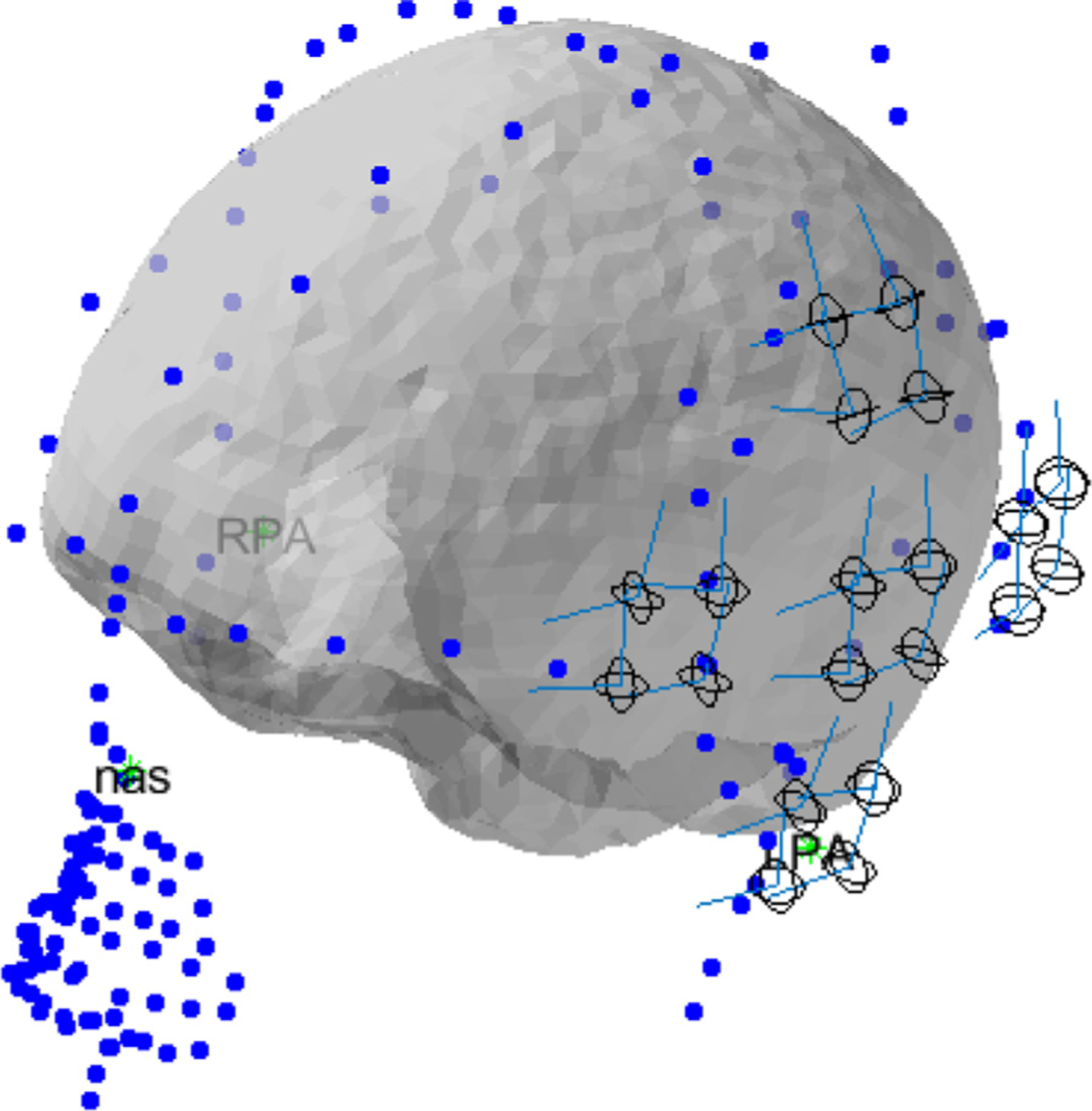
The simulated sensor array’s co-registration. The array covers the subject’s digitized scalp and their brain’s image obtained through MRI. The circles represent the OPM channel location.

3.4. Signal processing

For both simulation and experiment, we apply a sinusoidal signal at an arbitrary angle in the x -y plane and measure the phase and amplitude to determine the potential errors. To alleviate the effect of noise and limited sampling frequency, both the measured reference and the OPM signals are fitted with a sinusoidal function, as shown in Fig. 4. The sinusoidal function has a variable phase and amplitude, to be determined by non-linear optimization. The phase difference between the fitted reference and OPM signals is the induced phase shift.

Fig. 4.

Extracting phase and amplitude from the data. Both the coil driver signal and the OPM signal are fitted with a sinusoidal function. The difference between the zero crossings of the fitted functions (black arrow) portrays the phase difference.

4. Results and discussions

4.1. No cross-axis projection error: simulation vs experiment

To compare the numerical simulation to the experiment, we first evaluate results for the case of nulled magnetic field (B_z0 = 0) as shown in Fig. 5. For both simulation and experiment, the resolution of the rotating sinusoid is 1° as it rotates in the x -y plane with an amplitude of 0.33 nT and a frequency of 25 Hz. The result shown in Fig. 5 can be readily calculated using Eq. (3) (Cohen-Tannoudji et al., 1970), as the Larmor precession frequency (γB_z0 and γB_y0) is much smaller than the relaxation rate (1∕τ). The simulation and experiment yield almost identical results for the calculated amplitude and phase. There is a slight rotation in the sensitive axis between measurement and simulation which is attributed to a combination of uncompensated light-shift and remnant static magnetic field. Also, there is a 6° phase offset between the measurement and simulation which is attributed to difference in bandwidth between the OPM and the simulation. Nevertheless, simulation and experiment are in good agreement for both amplitude and phase calculations.

Fig. 5.

(a) Comparison of simulation (SIM) and experiment (MEAS) reults for the case of zero remnant magnetic field (B_z0 = 0). (b) Zoomed in for 180°-out-of-phase region. ∠α = 0 indicates the magnetic signal is alinged with the x-axis.

4.2. Cross-Axis projection error: simulation vs experiment

As described in the theory section, a static magnetic field in the direction of laser propagation (B_z0) causes CAPE in both phase and amplitude. By rotating the signal field under several different static magnetic field values in simulation, the effects of CAPE are clearly seen (Fig. 6-a and -b) for a 25 Hz sinusoidal signal. By increasing (decreasing) B_z0, the sensitive axis is rotated clockwise (counterclockwise); in other words, despite the fixed modulation axis, the sensitive axis orientation is rotated (3.33 °/nT) by the static magnetic field on the laser propagation axis (B_z0). Another important feature is that the amplitude response does not go to zero at 90° to the maximum response. Furthermore, as can be observed from the phase graph, Fig. 6-a, the minimum amplitude region corresponds to an expanded phase transition region that grows with the larger magnitude of B_z0; such expansion will result in zero crossing errors as will be discussed in subsequent sections. We find that the magnitude of the minimum response and the width of the phase transition region increase with the frequency of the signal. It is important to note that in simulations with B_z0 = 0 and B_y0 ≠ 0 that, while there is a rotation of the sensitive axis, the amplitude response does go to zero at 90° to the maximum response and there is not an expanded phase transition region. The OPM’s measured phase and amplitude are shown in Fig. 6-c and -d, respectively. These measurements reveal the same pattern as the simulation results. Specifically, both amplitude and phase graphs indicate that the sensitive axis is rotated clockwise (counterclockwise) by increasing (decreasing) the static magnetic field on the laser’s propagation axis (B_z0).

Fig. 6.

CAPE in the OPM for a 25 Hz, sinusoidal signal with an amplitude of 0.33 nT. Simulated phase (a) and normalized amplitude (b). Measured phase (c), and normalized amplitude (d). The legend refers to the magnitude of the static magnetic field on the laser propagtion axis (B_z0); B_x = cos(α) × sin(2π × 25 × t) and B_y = sin(α) × sin(2π × 25 × t).

The physical origin of CAPE arises from the longitudinal field (B_z0) causing the OPM to operate as low-field SERF OPM and a high-field OPM simultaneously. In a common instantiation of a high-field OPM, the pump laser aligns the atomic spins to a constant field (B_z0), and then a transverse field at the Larmor frequency $\left(\omega =\gamma B_{z0}/q\right)$ is applied to excite an electron spin resonance to tip the atomic spins away from the z-axis to precess about B_z0. When the frequency of the transverse field is swept about the Larmor frequency, the phase of the atomic response goes through a 180° phase shift (Groeger et al., 2006). For the case where B_z0 = 4.8 nT, the Larmor frequency is ∼27 Hz, and the zero-field resonance and the high-field resonance overlap. The atomic response to a signal frequency at 25 Hz is thus the combined response to both resonances. If the remnant field is along the y-axis, the geometry of the system does not allow the high-field resonance to be excited explaining why substantial phase shift effects are not seen for this configuration.

The amplitude error is calculated by taking the percentage of the difference between the normalized amplitude and the B_z0 = 0 nT case. The simulated amplitude error (Fig. 7-a) can be as large as 30% and will degrade accuracy in any imaging system employing OPMs. The amplitude error reaches its maxima for a magnetic field orthogonal (±90°) to the rotated sensitive axes. The measured amplitude error (Fig. 7-a) shows the same pattern as that of the simulation; however, the symmetry around the zero-gain point (±90°) is broken which is attributed to uncompensated remnant static magnetic field and remnant AC stark shift (Cohentannoudji and Dupontro, 1972) not accounted for in the simulation.

Fig. 7.

Simulated (a) and measured (b) amplitude error of the OPM caused by CAPE. The larger the B_z0 the larger the error. The error is calculated as the amplitude difference with the case of no remnant static magnetic field (B_z0 = 0). For signals in vicinity of α=90° the error can be as large as 30%. The asymmetry in the measured error is due to light shift.

The amplitude errors in Fig. 7 assume the sensitive axis is parallel to the modulated field B_m. However, these errors can be reduced by finding the maximum response to the field and determining a new angle for the sensitive axis as shown in Fig. 8. The rate of change in the sensitive axis orientation is 2.86 °/nT for the measured OPM data; the difference with the simulated value (3.33 °/nT) is mainly due to different total relaxation rates(l/τ), i.e. the sensor’s bandwidth.

Fig. 8.

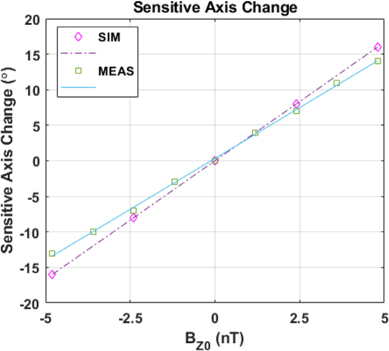
Measured change in the sensitive axis orientation (°) vs. the DC magnetic field on the laser’s propagation axis (B_z0) for a 25 Hz signal. CAPE rotates the sensitive axis by a measured gain of 2.86 °/nT and a simulated gain of 3.33 °/nT. The slight difference between the two is attributed to different relaxation rates.

The phase errors manifest as zero crossing errors, since the OPMs output phase, θ_OPM + θ_CAPE in Eq. (5), varies based on the static magnetic field on the laser propagation axis (B_z0) experienced by each sensor. The measured zero crossing error for a 16-ch OPM array is shown in Fig. 9. For this measurement a small-diameter coil, i.e. a magnetic dipole, is activated by a 25-Hz sinusoidal signal, and its magnetic field is captured by the OPM array. The OPM channels suffer from an uncompensated static magnetic field on the propagation axis of the laser (B_z0) up to ±1 nT. As it can be seen in the inset of Fig. 9, the channels have different phase which is attributed to CAPE. In wearable OPM-MEG systems the sensors conform to the subject’s head; hence, the sensors positions are calibrated on the fly using magnetic dipoles, i.e. head position indicator (HPI) coils, generating signals in the OPM bandwidth (Pfeiffer et al., 2018). To improve the accuracy of calibration procedures, the HPI coils generate a large magnetic field maximizing the SNR. In the presence of even small remnant magnetic field, the large magnetic fields generated by HPI coils will result in substantial CAPE-induced phase and gain error as shown in Fig. 9. Hence, the calibration accuracy of wearable OPM-MEG system is also impacted by CAPE.

Fig. 9.

Measured zero crossing error in OPM array; a 25 Hz magnetic dipole is activated and its signal is captured by a 16-ch OPM system. The inset displays the zero crossing attributed to expanded phase transition region due to CAPE.

CAPE not only impacts the artificially generated sinusoidal signals; it can severely degrade the fidelity of MEG signals as well. The somatosensory evoked magnetic field (SEF) response has a sharp peak at 20 ms (M20) with frequency contents of up to 80 Hz. In our SEF experiments (Borna et al., 2017), shown in Fig. 10, misalignment of channels’ peak response at 20 ms (M20) is evident. The peak misalignment was not resolved by considering the frequency response of individual channels, and one potential source is the CAPE; however, further investigation is needed to rule out other factors.

Fig. 10.

The misalignment of measured channels’ peak response at M20 SEF response. The observed misalignment could be stemmed from CAPE.

4.3. Cross-Axis projection error dependence on frequency: a simulation study

CAPE is highly dependent upon the frequency of the signal. Fig. 11 shows simulated CAPE-induced phase and amplitude for a fixed static magnetic field on the laser propagation axis (B_z0 = −4.8) and various signal frequencies. From the normalized amplitude graph of Fig. 11, the sensitive axis rotation is reduced for higher frequency signals converging to that of the ideal signal with no CAPE (B_z0 = 0). This can also be seen on the phase graph as well as a somewhat sharper phase transition for higher frequency signals. Hence, in the presence of static magnetic field, the sensitive axis is a function of frequency. By further processing the data of Fig. 11, the rate of change in sensitive axis rotation for various frequencies can be calculated as shown in Fig. 12. The sensitive axis is less impacted by remnant static magnetic field for high frequency signals. Nevertheless, as pointed out in section IV.B, and suggested by Fig. 12 the dependence of sensitive axis on frequency poses as a major problem for MEG systems as the brain-originated signals picked up by MEG systems cover a wide frequency range of 10–100 Hz (Hämäläinen et al., 1993) and also for calibration of wearable OPM-MEG sensors’ locations and gains.

Fig. 11.

CAPE-induced phase and normalized amplitude for various signal frequencies. B_z0 = −4.8 nT except for “No CAPE” which has B_z0 = 0 and a singal frequency of 5 Hz.

Fig. 12.

Rate of change in sensitive axis rotation for various frequencies. In the presence of remnant static magnetic field, the sensitive axis is frequency dependent and higher frequencies’ sensitive axes is less impacted by CAPE.

From the data in Fig. 11, one can infer the normalized amplitude error as the ratio of the minimum sensed amplitude to the sensed signal’s maximum amplitude for CAPE-free OPM. As can be observed in Fig. 13, the amplitude error is less than 1% for all frequencies when the remnant magnetic field is kept below ±1 nT. Furthermore, for larger remnant magnetic fields, the amplitude error has a bandpass characteristic; the low pass cut off frequency is defined by the OPM’s bandwidth with a high pass cut off frequency of about 8 Hz.

Fig. 13.

CAPE-induced amplitude error. The error is symmetric around B_z0 = 0, increases with magnitude of remnant field and has a bandpass dependency on signal frequency.

4.4. Impacts of OPM’s cross-axis projection error on the localization capability of magnetoencephalography systems

In magnetoencephalography systems employing OPMs (OPM-MEG), the calibration procedure is typically performed before brain imaging. Hence, the data collected during the MEG exam will be processed using the OPM sensors’ calibration data (gain, sensitive axis, channel location) acquired beforehand. The OPMs’ CAPE can potentially distort all the aforementioned calibration parameters. The OPMs’ CAPE is more pronounced in wearable OPM-MEG systems, where the OPM sensors can move. For sensors moving in a nonhomogeneous gradient magnetic field, their amplitude and phase will deviate from the ideal values, yielded by Eq. (6), based on the sensor-specific CAPE. Hence, the CAPE can detrimentally impact the source localization capability of all OPM-MEG systems. This section quantifies source localization error of OPM-MEG systems for the hypothetical scenario of random remnant DC magnetic field. Such remnant magnetic fields in the OPM sensor may arise from multiple mechanisms. For example, if slightly magnetized components are used in sensor construction, there can be random remnant static magnetic fields at each channel location, and it may be difficult to compensate the complex, near-field, magnetic patterns of the magnetized components. Another source of random remnant DC magnetic field is AC stark shift causing a fictitious magnetic field along the pump axis of various sensors.

To simulate the random B_z0 scenario, OPM channels are assigned a random static magnetic field on the laser propagation axis (B_z0) drawn from a normal Gaussian distribution with a varying standard deviation (σ). The random distribution is generated twenty times, and the results are averaged. Fig. 14 displays the mean and standard deviation (bars) of the source localization error while varying B_z0’s standard deviation (σ(B_z0)). As expected, the source localization error grows with increasing (B_z0). For (B_z0) as small as 10 nT, the induced average source localization error can be as large as 1 cm.

Fig. 14.

The mean and standard deviation (bars) for source localization error; the x-axis is the standard deviation of the remnant static magnetic field on the laser propagation axis selected from a normal gaussian distribution.

5. Conclusion

CAPE is an inherent error term in optically pumped magnetometer sensors, which manifests if the signal magnetic field has components along multiple axes of the OPM and is accompanied by a remnant static magnetic field perpendicular to the nominal sensitive axis. A remnant field along the OPM’s laser propagation axis is particularly detrimental because phase errors are also introduced. The magnitude of the remnant magnetic field found to introduce the error is well below the criteria for the spin-exchange-relaxation-free regime. Our simulation of a point-like OPM is in good agreement with our experimental results. Note that our simulation approximated the operating parameters (R_op and R_rel) for our sensor. Other OPMs operate under different conditions and may tolerate a larger or smaller remnant field range depending on the parameters of the OPM.

The impact of CAPE of an OPM-MEG system on MEG measurements is the introduction of time delays in signals in the typical MEG frequency band of interest and amplitude and orientation errors that effect source localization accuracy. In our simulation of source localization, the OPM array is configured for an auditory evoked magnetic field experiment and assumes quasistatic fields. If not taken into account, CAPE may diminish potential source localization advantages of OPMs over SQUIDs (Boto et al., 2016; Iivanainen et al., 2017). There are several strategies for mitigating the CAPE. First and most obvious, the remnant static fields can be nulled using a combination of large coils that surround the array and on-sensor coils that null fields from the sensor itself. Second, the orientation of the sensitive axis and the gain can be measured for each sensor. This is done routinely with our OPM array because the field modulation applied by the on-sensor coils for one sensor can interfere with the neighboring sensors (Borna et al., 2017). However, it should be emphasized that this method works for stationary array where the remnant magnetic field is relatively constant for the duration of experiment. With a measurement of the sensitive axis, both CAPE and sensor-to-sensor interference effects can be minimized. Finally, active feedback using coils within each sensor can continuously minimize the field. This is an attractive solution because CAPE is effectively eliminated, but substantial development is required to make a triaxial sensor (Shah, 2021) and to ensure fields from neighboring sensors do not interfere with each other, which could induce unstable feedback conditions and crosstalk (Nardelli et al., 2019). Calibration and characterization of an OPM-MEG sensor array is critical for MEG analyses such as neuronal source localization. One calibration method for determining the location and orientation of the OPM channels is to measure a known distribution of small coils or an MEG phantom. Care should be taken to keep the signal amplitudes low, and when analyzing the applied signals, we find it necessary to eliminate channels showing large phase errors with respect to the current signal since they are most likely suffering from gain errors as well. This is an effective method to improve the accuracy of calibration routines in the presence of CAPE. The aforementioned techniques are most easily implemented in stationary OPM arrays. However, wearable OPM-MEG arrays are a compelling new paradigm (Boto et al., 2016) for MEG where CAPE must be addressed. The sensors of wearable OPM-MEG systems continuously change their angle relative to a remnant static magnetic field if the field is not nulled properly. Substantial strides have been made in cancelling the remnant fields within a magnetically shielded room (Holmes et al., 2018). Based on our simulation and experimental results if the remnant field is kept below ±1 nT, CAPE effects are likely sufficiently small for most MEG measurements, but we caution this should be verified for high precision measurements. Nevertheless, we believe continued development in OPM and field nulling technology will mitigate the effects of CAPE and sensor-to-sensor interference to enable the predicted advantages of OPM-base MEG measurements.

References

- Borna A, Carter TR, Colombo AP, Jau YY, McKay J, Weisend M, Taulu S, Stephen JM, Schwindt PDD, 2020. Non-invasive functional-brain-imaging with an OPM-based magnetoencephalography system. PLoS ONE 15 (1), e0227684. [DOI] [PMC free article] [PubMed] [Google Scholar]
- Borna A, Carter TR, Goldberg JD, Colombo AP, Jau YY, Berry C, McKay J, Stephen J, Weisend M, Schwindt PDD, 2017. A 20-channel magnetoencephalography system based on optically pumped magnetometers. Phys. Med. Biol 62 (23), 8909–8923. [DOI] [PMC free article] [PubMed] [Google Scholar]
- Boto E, Bowtell R, Kruger P, Fromhold TM, Morris PG, Meyer SS, Barnes GR, Brookes MJ, 2016. On the potential of a new generation of magnetometers for MEG: a beamformer simulation study. PLoS ONE 11 (8). [DOI] [PMC free article] [PubMed] [Google Scholar]
- Boto E, Holmes N, Leggett J, Roberts G, Shah V, Meyer SS, Munoz LD, Mullinger KJ, Tierney TM, Bestmann S, Barnes GR, Bowtell R, Brookes MJ, 2018. Moving magnetoencephalography towards real-world applications with a wearable system. Nature 555 (7698), 657 -+. [DOI] [PMC free article] [PubMed] [Google Scholar]
- Cohen-Tannoudji C, Dupont-Roc J, Haroche S, Laloë FJRPA, 1970. Diverses résonances de croisement de niveaux sur des atomes pompés optiquement en champ nul. I. Théorie 5 (1), 95–101. [Google Scholar]
- Cohentannoudji C, Dupontro J, 1972. Experimental study of Zeeman light shifts in weak magnetic-fields. Phys. Rev. A Gener. Phys 5 (2), 968 -+. [Google Scholar]
- Colombo AP, Carter TR, Borna A, Jau Y−Y, Johnson CN, Dagel AL, Schwindt PDD, 2016. Four-channel optically pumped atomic magnetometer for magnetoencephalography. Opt. Express 24 (14), 15403–15416. [DOI] [PMC free article] [PubMed] [Google Scholar]
- Groeger S, Bison G, Schenker JL, Wynands R, Weis A, 2006. A high-sensitivity laser-pumped Mx magnetometer. Eur. Phys. J. D Atom. Mol. Opt. Plasma Phys 38 (2), 239–247. [Google Scholar]
- Hämäläinen M, Hari R, Ilmoniemi RJ, Knuutila J, Lounasmaa OV, 1993. Magnetoencephalography-theory, instrumentation, and applications to noninvasive studies of the working human brain. Rev. Mod. Phys 65 (2), 413–497. [Google Scholar]
- Happer W, Jau YY, Walker T, 2010. Optically Pumped Atoms Wiley. [Google Scholar]
- Holmes N, Leggett J, Boto E, Roberts G, Hill RM, Tierney TM, Shah V, Barnes GR, Brookes MJ, Bowtell R, 2018. A bi-planar coil system for nulling background magnetic fields in scalp mounted magnetoencephalography. Neuroimage 181, 760–774. [DOI] [PMC free article] [PubMed] [Google Scholar]
- Iivanainen J, Stenroos M, Parkkonen L, 2017. Measuring MEG closer to the brain: performance of on-scalp sensor arrays. Neuroimage 147, 542–553. [DOI] [PMC free article] [PubMed] [Google Scholar]
- Iivanainen J, Zetter R, Gron M, Hakkarainen K, Parkkonen L, 2019. On-scalp MEG system utilizing an actively shielded array of optically-pumped magnetometers. Neuroimage 194, 244–258. [DOI] [PMC free article] [PubMed] [Google Scholar]
- Iivanainen J, Zetter R, Parkkonen L, 2020. Potential of on-scalp MEG: robust detection of human visual gamma-band responses. Hum. Brain Mapp 41 (1), 150–161. [DOI] [PMC free article] [PubMed] [Google Scholar]
- Jau YY, 2005. Unpublished Pedagogical Note Princeton University. [Google Scholar]
- Johnson C, Schwindt PDD, Weisend M, 2010. Magnetoencephalography with a two–color pump-probe, fiber-coupled atomic magnetometer. Appl. Phys. Lett 97 (24). [Google Scholar]
- Knappe S, Mhaskar R, Preusser J, Kitching J, Trahms L, Sander T, 2012. Chip-scale room-temperature atomic magnetometers for biomedical measurements. In: Proceedings of the 5th European Conference of the International Federation for Medical and Biological Engineering, Pts 1 and 2 37, pp. 1330–1333. [Google Scholar]
- Kominis IK, Kornack TW, Allred JC, Romalis MV, 2003. A subfemtotesla multichannel atomic magnetometer. Nature 422, 596–599. [DOI] [PubMed] [Google Scholar]
- Nardelli NV, Krzyzewski SP, Knappe SA, 2019. Reducing crosstalk in optically-pumped magnetometer arrays. Phys. Med. Biol 64 (21), 21NT03. [DOI] [PubMed] [Google Scholar]
- Nardelli NV, Perry AR, Krzyzewski SP, Knappe SA, 2020. A conformal array of microfabricated optically-pumped first-order gradiometers for magnetoencephalography. Epj. Quantum Technol 7 (1). [Google Scholar]
- Nolte G, 2003. The magnetic lead field theorem in the quasi-static approximation and its use for magnetoencephalography forward calculation in realistic volume conductors. Phys. Med. Biol 48 (22), 3637–3652. [DOI] [PubMed] [Google Scholar]
- Oostenveld R, Fries P, Maris E, Schoffelen J−M, 2011. FieldTrip: open source software for advanced analysis of MEG, EEG, and invasive electrophysiological data. Comput. Intell. Neurosci 2011, 9. [DOI] [PMC free article] [PubMed] [Google Scholar]
- Pfeiffer C, Andersen LM, Lundqvist D, Hämäläinen M, Schneiderman JF, Oostenveld R, 2018. Localizing on-scalp MEG sensors using an array of magnetic dipole coils. PLoS ONE 13 (5), e0191111–e0191111. [DOI] [PMC free article] [PubMed] [Google Scholar]
- Savukov I, Romalis M, 2005. Effects of spin-exchange collisions in a high-density alkali-metal vapor in low magnetic fields. Phys. Rev. A 71 (2). [Google Scholar]
- Scofield JH, 1994. Frequency-domain description of a lock-in amplifier. Am. J. Phys 62 (2), 129–133. [Google Scholar]
- Seltzer SJ, 2008. Developments in Alkali-Metal Atomic Magnetometry Princeton Ph.D.
- Seltzer SJ, Romalis MV, 2004. Unshielded three-axis vector operation of a spin-exchange-relaxation-free atomic magnetometer. Appl. Phys. Lett 85 (20), 4804–4806. [Google Scholar]
- Shah V (2021). “Triaxial OPM” from https://quspin.com/new-triaxial-qzfm/.
- Shah VK, Wakai RT, 2013. A compact, high performance atomic magnetometer for biomedical applications. Phys. Med. Biol 58 (22), 8153–8161. [DOI] [PMC free article] [PubMed] [Google Scholar]
- Xia H, Baranga ABA, Hoffman D, Romalis MV, 2006. Magnetoencephalography with an atomic magnetometer. Appl. Phys. Lett 89 (21), 211104. [Google Scholar]
- Zimmerman JE, Thiene P, Harding JT, 1970. Design and operation of stable RF-biased superconducting point-contact quantum devices, and a note on properties of perfectly clean metal contacts. J. Appl. Phys 41 (4), 1572 -+. [Google Scholar]
Associated Data
This section collects any data citations, data availability statements, or supplementary materials included in this article.