

Abstract
The functional connectomic profile is one of the non-invasive imaging biomarkers in the computer-assisted diagnostic system for many neuro-diseases. However, the diagnostic power of functional connectivity is challenged by mixed frequency-specific neuronal oscillations in the brain, which makes the single Functional Connectivity Network (FCN) often underpowered to capture the disease-related functional patterns. To address this challenge, we propose a novel functional connectivity analysis framework to conduct joint feature learning and personalized disease diagnosis, in a semi-supervised manner, aiming at focusing on putative multi-band functional connectivity biomarkers from functional neuroimaging data. Specifically, we first decompose the Blood Oxygenation Level Dependent (BOLD) signals into multiple frequency bands by the discrete wavelet transform, and then cast the alignment of all fully-connected FCNs derived from multiple frequency bands into a parameter-free multi-band fusion model. The proposed fusion model fuses all fully-connected FCNs to obtain a sparsely-connected FCN (sparse FCN for short) for each individual subject, as well as lets each sparse FCN be close to its neighbored sparse FCNs and be far away from its furthest sparse FCNs. Furthermore, we employ the ℓ1-SVM to conduct joint brain region selection and disease diagnosis. Finally, we evaluate the effectiveness of our proposed framework on various neuro-diseases, i.e., Fronto-Temporal Dementia (FTD), Obsessive-Compulsive Disorder (OCD), and Alzheimer’s Disease (AD), and the experimental results demonstrate that our framework shows more reasonable results, compared to state-of-the-art methods, in terms of classification performance and the selected brain regions. The source code can be visited by the url https://github.com/reynard-hu/mbbna.
Keywords: Functional connectivity, semi-supervised learning, neuro-disease diagnosis, resting state fMRI
I. Introduction
RESTING state functional Magnetic Resonance Imaging (fMRI) has been verified to have the potential of improving neuro-disease diagnosis by constructing Functionally Connectivity brain Networks (FCNs) [1], [2]. It results in a comprehensive understanding of neurological disorders at a whole-brain level by measuring synchronized time-dependent changes in the Blood Oxygenation Level Dependent (BOLD) signals [3], [4]. Hence, fMRI has been becoming a valuable technique for identifying biomarkers with neuroimaging data.
Correlation-based methods are commonly used to construct fully-connected FCNs, where each node (i.e., one brain region) connects with all nodes and each edge measures the synchronization degree of functional activities [5], [6]. Traditional Pearson correlation analysis only captures pairwise information and thus is vulnerable to spurious or insignificant functional connectivities. Recently, sparse methods in [7]–[9] were proposed to construct sparsely-connected FCNs (sparse FCN for short), where each node connects with a part of nodes to reduce the influence of unreal or unimportant functional connections. However, previous methods for neuro-disease analysis on fMRI data, such as Pearson correlation analysis and sparse methods, still have to face many challenges due to the reasons, including heterogeneity across subjects, the curse of dimensionality, noise influence, inter-subject variability, etc.
In search of significant disease diagnosis, there is a consensus that BOLD signal only contains a small portion of frequencies (i.e., 0.01-0.08HZ) that are related to neural activity [10], [11]. Based on this observation of fMRI, current computational methods characterize the full connectivity using the filtered BOLD signals where some frequency bands of the signals have been filtered, with the assumption that the filtered BOLD signals can reflect the complex brain functions for all brain regions [12]. As a complex system, however, each brain region consists of functionally similar neurons that support differentiable functions. In this regard, one possible solution would be fine-tuning the BOLD signals into a fine-grained frequency band tailored to the brain function of subspecialized brain regions. Since the exact definition of brain function in each region is still largely under debate [13], the alternative solution is to disentangle the heterogeneity in BOLD signals. Specifically, the BOLD signals are first decomposed into multiple frequency bands (multi-band for short) based on the characteristics of full connectivity. The multi-band signals are then fused into a unified region with adaptively full connectivity representation, which can significantly enhance the diagnostic power of connectivity biomarkers for the computer-assisted diagnosis.
After obtaining multiple fully-connected FCNs for each subject, it is necessary to combine them into a common fully-connected or sparse FCN, aiming at learning the most representative features across individuals (or subjects). However, different frequency bands of neuronal signals usually carry unique functional information, which is different from others to support differentiable functions [13], i.e., band diversity for short. Hence, it is unreasonable to construct a common FCN by averaging different frequency bands for each subject. Moreover, it is difficult to align FCNs across subjects due to the heterogeneity across subjects.
In this paper, we hypothesize that the observed brain activity is a mixture of harmonic signals with different frequency bands and the dysfunction patterns of different brain disorders have different responses in different frequency bands, and thus propose a functional connectivity analysis framework to jointly conduct feature learning and personalized disease diagnosis with fMRI data, in a semi-supervised manner. Specifically, the proposed framework is listed in Fig. 1 by involving the following key steps. (1) We first apply the wavelet toward the mean time courses on each brain region to obtain the wavelet coefficient at each frequency, and further employ the conventional Pearson correlation analysis to obtain a fully-connected FCN for each subject at the underlying frequency. (2) We investigate a parameter-free multi-band fusion method to automatically output a sparse FCN by fusing multiple fully-connected FCNs for each subject, as well as to let each sparse FCN be close to its near sparse FCNs and be far away from its furthest sparse FCNs. (3) We employ the ℓ1-SVM to jointly select brain regions (i.e., feature selection) and conduct disease diagnosis (i.e., classification).
Fig. 1.
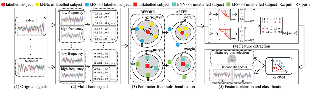
The proposed framework for functional neuroimaging biomarker identification: (1) Original Blood Oxygenation Level Dependent (BOLD) signals for M subjects; (2) Each signal was first partitioned into multi-band signals (e.g., a low frequency signal and a high frequency signal) using the Discrete Wavelet Transform (DWT) method and the Pearson correlation coefficient was then calculated on each frequency band signal to obtain the fully-connected Functionally Connectivity brain Networks (FCNs); (3) The proposed parameter-free multi-band fusion model is designed to automatically learn a sparse FCN Sm (m = 1, …, M) by fusing multiple fully-connected FCNs for each subject, as well as to learn sparse FCNs for all subjects by pulling each sparse FCN to be close to its k nearest neighbors (kNNs) and pushing each subject to be far away from its k furthest sparse FCNs (kFSs); (4) A data matrix X is obtained by extracting the upper triangle part of Sm; (5) The ℒ1-SVM is employed to jointly construct feature selection (i.e., the connection between two brain regions) and the classification task (i.e., disease diagnosis).
II. Method
Assume we have M subjects and each subject has the BOLD signal (m = 1, …, M) where n and t, respectively, represent the number of brain regions and the length of signals, we denote (v = 1, …, V) as the fully-connected FCN of the v-th band signal of the m-th subject obtained by Pearson correlation analysis on n brain regions, this work investigates to learn a common sparse FCN for each subject so that Sm could fuse the functional connectivity from V fully-connected FCNs Am,v, as well as is close to its neighbors and is far away from its furthest sparse FCNs. As a result, it is homogeneous to other sparse FCNs.
A. Multi-Band Signals
Conventional methods of functional connectivity using fMRI data focused on characterizing BOLD signals with low frequency range (generally from 0.01 to 0.08HZ) [5], [14], [15]. In particular, the signals within the frequency range close to 0.00HZ are more likely to be affected by the periodically noisy signals generated by the undersampled periodic hardware [8], [15], the signals within the frequency range in 0.00-0.01HZ are significantly related to non-physiologic origin (i.e., the MRI scanner drift) and are usually treated as covariates of no interest in the statistical analysis [16]. Therefore, the removal of the signals within the frequency range of [0.00HZ, 0.01HZ] ensures that the obtained BOLD signals are predominately related to the physiological state. Furthermore, the removal of the signals above 0.08HZ can minimize the interference of other external signals [17]. Recently, studies demonstrated that the dysfunctional patterns affecting the neuro-diseases are the mixture of brain activity with multiple frequency bands [13]. Due to the complexity of human brains, the frequency band usually dominates the subtle functional patterns that are specific to certain disorders. Even under the resting state, the complexity of brain activity is beyond the power of single frequency band [18]. In addition, the changes across different frequency bands (i.e., band diversity) have been known little [12], [19]. Hence, it is challenging to consider multiple frequency bands for neuro-disease analysis with fMRI data.
B. Sparse FCN Learning
We employ Pearson correlation analysis to obtain V fully-connected FCNs using multi-band signals. However, there are at least two issues that need to be addressed, i.e., band diversity and FCN’s interpretability.
First, band diversity indicates that different band signals contain different characteristics, as shown in Fig. 2, where either the low frequency band signal or the high frequency band signal has different information, compared to the original signal which is a mixture of the low frequency band signal and the high frequency band signal. Moreover, the low frequency band and the high frequency band have complementary information to each other. For example, the solid yellow rectangle in the low frequency band signal (i.e., the second red dot rectangle) is unclear as well as small, while the solid yellow rectangle in the high frequency band signal is clear as well as big, similar to the original signal in Fig. 2. Both the difference and the complementary between the low frequency band signals and the high frequency band signals motivate us to first decompose them and then to fuse them, as shown in Fig. 2, where our proposed multi-band signal removes the noise (i.e., correlations are far away from the diagonal) as well as clearly preserves the local structures (i.e., five red dot rectangles across the diagonal).
Fig. 2.
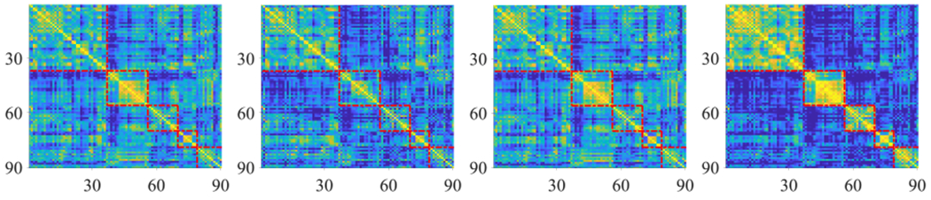
Visualization of correlation analysis of a signal from the data set FTD with different frequency bands, i.e., the original signal, the low frequency band signal, the high frequency band signal, and the multi-band signal, from left to right.
The second drawback of the fully-connected FCN is the lack of interpretability. Moreover, its connectivity may contain noise (e.g., either irrelevant or spurious connectivities) to possibly affect the analysis of brain networks [20], [21]. Neurologically, a certain brain activity or a specific disease predominantly interacted with a part of brain regions. Therefore, the sparse connectivities are preferred to construct brain connectivity networks [9].
Given multiple fully-connected FCNs for an individual subject, by considering the band diversity of every signal and the interpretability of every fully-connected FCN, in this paper, we investigate to fuse the fully-connected FCNs of every subject to a sparse FCN by
| (1) |
where ‖·‖F represents the Frobenius norm and α is a non-negative tuning parameter. is the penalty or constraint on Sm (m = 1, …, M). and , respectively, represent the i-the row of Sm and the i-th row and the j-th column element of Sm. 1 and , respectively, indicate the all-one-element vector and the nearest neighbor set of the i-th brain region. The constraint “ if , other wise 0” implies that each node is sparsely represented by other nodes (i ≠ j, i, j = 1, …, n).
Compared to previous methods, Eq. (1) has the following advantages. First, Eq. (1) aims at obtaining a sparse FCN Sm for the m-th subject based on V fully-connected FCNs Am,v (v = 1, …, V) by considering the band diversity. Second, the new representation Sm is iteratively updated by Eq. (1). Specifically, the value of Sm can be adjusted with the updated Sm′ (m ≠ m′). It is noteworthy that previous methods (e.g., sparse coding [22] and sparse graph [9]) generate unchanged FCNs. Third, the sparse number for each row of Sm varies based on the data distribution. Specifically, the connectivity number (i.e., the non-zero number for each row) for each node is automatically decided by Lemma 2 in Section II-E.
Finally, we list our motivation of fusing information across different frequency bands as well as different subjects in Eq. (1) as follows.
First, different frequency bands of the signals contain different important information and noise, so it is intuitive and popular to combine multi-source data (i.e., the information across different frequency bands in this work) together to obtain discriminative representations in the domains of machine learning and medical image analysis. To achieve this, Eq. (1) learns a common sparse representation Sm (m = 1, …, M) for each subject by fusing multiple fully-connected FCNs Am,v (v = 1, …, V) collected from different frequency bands.
Second, if the representation of each subject is obtained independently, the obtained representation Sm for the m-th subject is easily heterogeneous to other representations Sm′ (m ≠ m′). Eq. (1) learns the representations of all subjects in the same framework by using the regularization term defined in Section II-C, aiming at learning homogenous representations for all subjects. Moreover, minimizing the error across all subjects is to learn a common sparsely-connected representation Sm for each subject as well as to generate homogeneous representations for all subjects. In the literature, minimizing the error across all subjects is popular. For example, Hinrich et al. proposed minimizing the error of negative log-likelihood across subjects to ensure the temporal components from a consistent set of brain regions [23].
As a result, Eq. (1) considers the fusion across frequency bands as well as all subjects simultaneously to output discriminative and homogenous representations for all subjects. Physiologically, the fusion in Eq. (1) can explore the discriminative information implicitly across frequency bands [24], and can enhance data consistency across subjects [25].
C. Parameter-Free Multi-Band Fusion
Without taking the constraint into account, the optimization of Sm is independent on the optimization of Sm′ (m ≠ m′). This may output trivial solutions for Sm, i.e., the average of Am,v (v = 1, …, V). To solve this issue, we define the constraint in Eq. (1) based on the following observations.
First, in real applications, the BOLD signals usually come from different places such as different hospitals and different machines, so the fully-connected FCNs are easily heterogeneous to each other, i.e., heterogeneity across subjects. It is straightforward to smooth all FCNs so that they are homogeneous. Second, in our proposed personalized classifier, the training set includes labelled subjects and unlabelled subjects. Specifically, given a test subject, the personalized framework makes full use of all labelled subjects and unlabelled subjects to construct the learning model, and thus it is exactly a semi-supervised manner. Hence, it is very helpful if the outputted Sm has significant discriminative ability.
Weinberger and Saul proposed a supervised Large Margin Nearest Neighbor (LMNN) to conduct metric learning by keeping the local neighborhood of the training subjects [26], i.e., the neighbors of each subject in the new feature space are exactly its original neighbors in the original feature space. Specifically, the first term of the LMNN penalizes large distances between each subject and its original neighbors with the same label, and its second term penalizes the small distances of the subjects with different labels. As a result, the labelled subjects are close to the subjects with the same label and are far away from the subjects with different labels. In this way, the LMNN classifier has discriminative ability. However, LMNN was designed for metric learning and did not consider the discriminative ability of unlabelled subjects.
In this work, considering the semi-supervised scenario where the training subjects include labelled subjects and unlabelled subjects, we first have an observation that the k nearest neighbor (kNN) classifier always classifies subjects to the class of their nearest neighbors. Hence, each subject (either a labelled subject or an unlabelled subject) should share the same label with its kNNs and should have different labels to its distant subjects. More specifically, by denoting “k nearest neighbors” and “k furthest subjects”, respectively, as “kNNs” and “kFSs”, the set of labelled subjects and the set of unlabelled subjects, as and , respectively, we define the neighbor set and the distant set as follows:
Definition 1: of the i-th unlabelled subject includes its kNNs in , and of the i-th labelled subject includes its kNNs with the same label in , i.e.,
| (2) |
Definition 2: of the i-th unlabelled subject includes its kFSs in , and of the i-th labelled subject includes its kFSs with different labels in , i.e.,
| (3) |
We then define as
| (4) |
where [.]+ = max(., 0) and β is a non-negative tuning parameter. In Eq. (4), the first term penalizes the large distance between Sm and its nearest neighbors in N(m). Specifically, the first term pulls Sm to approximate the average of its nearest neighbors or pulls them (i.e., Sm and its nearest neighbors) together. The second term pushes the Sm against its furthest subjects in so that their distance is larger than a fixed margin, i.e., at least a unit “1” in Eq. (4), as shown in the third part of Fig. 1. In this way, the sparsely-connected representation of FCN Sm is dependent on others Sm′ (m ≠ m′) as well as contains the discriminative ability, i.e., having a fixed margin to its furthest subjects as well as being close to its nearest neighbors as much as possible, which benefits avoiding the influence of outliers.
Considering Eq. (1) and Eq. (4), the multi-band fusion model in Eq. (1) needs to tune the parameter α, which is time-consuming and needs prior knowledge. In particular, as a personalized framework which trains a fusion model for every test subject, the tuning of parameters is time-consuming. To address this issue, we propose a parameter-free multi-band fusion model as follows:
| (5) |
Compared Eq. (5) with Eq. (1), Eq. (5) uses a square root operator on the fusion error of each subject to replace the parameter a in Eq. (1). Specifically, when we conduct the derivative with respect to Sm, we always get
| (6a) |
where λ = [λ1, …, λM]. Eq. (6) is equivalent to Eq. (5) for the optimization of Sm (m = 1, …, M). That is, Eq. (5) does not need to tune the parameter by iteratively updating Eq. (6a) and Eq. (6b) to automatically obtain λm during the optimization process. λm can be regarded as an implicit parameter, rather than selecting the best one out of a range of values with cross-validation methods used in Eq. (1). The value of λm is exactly the weight of each subject, indicating the inter-subject variability of each subject. Compared Eq. (6) with Eq. (1), we have λm = 1/α for the optimization of the m-th FCN Sm. Hence, Eq. (1) uses a fixed parameter α while Eq. (6) uses a dynamic and data-driven parameter λm based on the data distribution.
After optimizing Eq. (5), we obtain smooth and sparsely-connected representation FCNs Sm (m = 1, …, M) by fusing multiple fully-connected FCNs Am,v (v = 1, …, V) into a common space. Such a space is spanned by Sm through its first term as well as shrinks the heterogeneity across subjects through its second term. Moreover, the second term can avoid the influence of outliers by keeping a margin between the nearest neighbor set and the furthest subject set for each subject. Furthermore, we transfer the optimization of Eq. (5) to Eq. (6) to obtain the trade-off between two terms by considering the inter-subject variability. Hence, Sm (m = 1, …, M) is the new representation of original BOLD signals.
D. Joint Region Selection and Disease Diagnosis
Since the new representation Sm (m = 1, …, M) is the matrix representation, it is difficult for using traditional classification methods to conduct disease diagnosis. In this work, we first convert Sm to a symmetric matrix through a formula Sm = (Sm + (Sm)T)/2, and then follow [9] to transfer the matrix representation to its vector representation, i.e., extracting the upper triangle part of the symmetric matrix Sm (m = 1, …, M) to form a row vector . In this way, we have the data matrix and the corresponding label vector y ∈ {−1, 1}M×1.
Many previous studies (e.g., [9], [27]) employed a two-stage strategy to conduct disease diagnosis, i.e., feature selection and disease diagnosis. Specifically, in these methods, feature selection is separated from disease diagnosis. Moreover, the goal of feature selection is to preserve the original information as much as possible, rather than to achieve high performance of disease diagnosis. As a result, the best results of feature selection are not good for disease diagnosis. On the contrary, the ℓ1-SVM (optimized by the public toolbox LIBLINEAR [28]) embeds feature selection by the ℓ1-norm regularization term on the coefficient matrix with the SVM classifier in the united framework. As a result, the results of feature selection are adjusted based on the classifier updated in the last iteration, while the classifier is also adjusted by the updated results of feature selection. In this way, the results of feature selection contribute to the construction of the classifier. Hence, the ℓ1-SVM can overcome the drawback of the two-stage strategy in previous methods.
It is noteworthy that the parameter-free multi-band fusion model uses both labelled subjects and unlabelled subjects while the process of joint feature selection and disease diagnosis uses the labelled subjects in the training process.
E. Optimization, Initialization, Complexity and Convergence
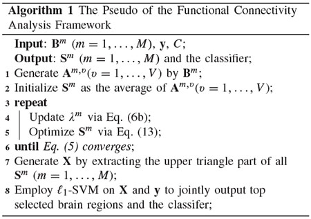
1). Optimization:
The proposed objective function in Eq. (5) is not convex for all variables, but is convex for any single variable while fixing other variables. Hence, in this paper, we employ the alternating optimization strategy [29] to iteratively update M FCNs Sm (m = 1, …, M) in Eq. (5) and list the pseudo of our proposed framework for functional connectivity analysis in Algorithm 1.
First, we obtain the expansion formula about Sm of the first term in Eq. (6a) as , and then obtain the expansion result of the second term about Sm in Eq. (6a) as
| (7) |
where , and k is the defined number of neighbors for each sample. The optimization of each row i = 1, …, n, in Sm is independent on other rows (i ≠ i′), so we list the optimization details of as follows.
| (8) |
where
| (9) |
where and . After finishing mathematical transformation, we have
| (10) |
where
| (11) |
where is a vector. The Lagrangian function with respect to is
| (12) |
where is the Lagrange multiplier and is a non-negative vector. Based on the complementary slackness of the Karush-Kuhn-Tucker (KKT) conditions [30], we have the closed-form solution of is
| (13) |
where is the j-th element of . The value of the Lagrange multiplier σ can be obtained by Lemma 1 from [31].
Lemma 1: By denoting the optimal solution in Eq. (13), letting r and u be two indices, and , only if , then must be equal to zero.
Based on Lemma 1, we can find some integers I = [ρ], 1 ≤ ρ ≤ n to meet the non-zero components of the sorted optimal solutions, i.e.,
| (14) |
As a result, the optimal values in can be described as , where the value of the optimal ρ is automatically obtained by Lemma 2 from [31].
Lemma 2: Let η represents the vector after sorting in a descending order, the number of strictly non-negative elements in is , i ∈ [n].
Based on Lemma 2, the non-zero number in the i-th row , i.e., the number of brain regions connected to the i-th brain region, is different from the non-zero number in the j-th row (i ≠ j). It is noteworthy that previous sparse methods set the same number of brain regions connected to each brain region. Obviously, our method is more flexible, compared to previous methods in [22], [32], [33].
Furthermore, Eq. (5) iteratively updates Eq. (6a) and Eq. (6b) based on the alternating optimization strategy [29], which has been proved to achieve convergence. Hence, the proposed parameter-free multi-band fusion model converges, while the ℓ1-SVM also converges.
2). Initialization:
In Algorithm 1, we initialize Sm as the average of Am,v(v = 1, …, V), which results in that the optimization of Eq. (5) converges within tens of iterations. Moreover, the result of Eq. (5) is insensitive to the initialization of Sm.
3). Complexity:
The generation of both multi-band signals and the fully-connected FCNs can be finished offline. The parameter-free multi-band fusion model takes a closed-form solution to optimize Sm (m = 1, …, M). Its time complexity is O(Mn2) where M and n, respectively, represent the number of the subjects and the number of brain regions. That is, the time complexity of our multi-band fusion model is linear to the subject size. Moreover, our model only stores Sm (m = 1, …, M) in the memory with the space complexity O (Mn2). The time complexity of ℓ1-SVM is linear to the subject size, while its space complexity is O (Mn(n – 1)/2) [28].
4). Convergence Analysis:
First, we follow the literature [34], [35] to have the following Lemma:
Lemma 3: The inequality
| (15) |
holds for non-negative values u and w.
Second, Theorem 3 proves the convergence of Algorithm 1:
Theorem 1: The objective function value of Eq. (5) monotonically decreases until Algorithm 1 converges.
Proof: After obtaining the optimal Sm(t) in the t-th iteration, we need to optimize Sm(t+1) in the (t + 1)-th iteration by fixing other Sm′(t) where m’ ≠ m, m = 1, …, M.
According to Eq. (13), has a closed-form solution for all i, j = 1, …, n, so we combine with Eq. (13) to have:
| (16) |
Based on Lemma 3, we obtain:
| (17) |
Combining Eq. (16) with Eq. (17), we have:
| (18) |
Hence, Eq. (18) demonstrates Algorithm 1 decreases the objective function value of Eq. (5) for every iteration until it converges. Therefore, the proof of Theorem 3 is completed.
III. Experiments
We experimentally evaluated our method, compared to four comparison methods, on three real neuro-disease data sets with fMRI data, in terms of binary classification performance.
A. Data Preparation
The data set fronto-temporal dementia (FTD) contains 95 FTD subjects and 86 age-matched healthy control (HC) subjects, from the recent NIFD database,1 managed by the frontotemporal lobar degeneration neuroimaging initiative. The data set obsessive-compulsive disorder (OCD) from Guangzhou Psychiatric Hospital [36] has 20 HC subjects and 62 OCD subjects. The data set Alzheimer’s Disease Neuroimaging Initiative (ADNI)2 includes 59 Alzheimer’s disease (AD) subjects and 48 HC subjects. The demographic information of all data sets is shown in Table I.
TABLE I.
Demographic Information for Three Data Sets. FTD: Fronto-Temporal Dementia; OCD: Obsessive-Compulsive Disorder; ADNI: Alzheimer’s Disease Neuroimaging Initiative; AD: Alzheimer’s Disease; HC: Healthy Controls
| Data sites | Age range (years) | Subjects | Time points (seconds) | Voxel size (mm3) | TR(ms) | Scanner | Field strength |
|---|---|---|---|---|---|---|---|
| FTD | 65-88 | 95 FTD; 86 HC | 230 | 3×3×3 | 2000 | Multi-site | 1.5/3T |
| OCD | 18-50 | 62 OCD; 20 HC | 230 | 3×3×3 | 2000 | Philips | 3T |
| ADNI | 57-82 | 59 AD; 48 HC | 120 | 3×3×3 | 2000 | Multi-site | 1.5/3T |
1). Data Set OCD:
a). Imaging data acquisition:
A 3.0-Tesla MR system (Philips Medical Systems, USA) equipped with an eight-channel phased-array head coil was used for data acquisition. Functional data were collected using gradient echo Echo-Planar Imaging (EPI) sequences (time repetition, TR = 2000ms; echo time, TE = 60ms; flip angle = 90°, 33 slices, field of view [FOV] = 240mm × 240mm, matrix = 64 × 64; slice thickness = 4.0mm). For spatial normalization and localization, a high-resolution T1-weighted anatomical image was acquired using a magnetization prepared gradient echo sequence (TR = 8ms, TE = 1.7ms, flip angle = 20°, FOV = 240mm × 240mm, matrix = 256 × 256, slice thickness = 1.0mm). During the scanning, participants were instructed to relax with their eyes closed, and stay awake without moving.
b). Functional imaging data preprocessing:
The data were preprocessed using the Statistical Parametric Mapping toolbox (SPM12)3 and Data Processing Assistant for Resting-State fMRI (DPARSFA version 4.4).4 Image preprocessing consisted of: 1) slice timing correction; 2) head motion correction; 3) realignment with the corresponding T1-volume; 4) nuisance covariate regression (six head motion parameters, white matte signal and cerebrospinal fluid signal); 5) spatial normalization into the stereotactic space of the Montreal Neurological Institute and resampling at 3 × 3 × 3 mm3; 6) spatial smoothing with a 6-mm full-width half-maximum isotropic Gaussian kernel; 7) band-pass filtering (0.01–0.08HZ); 8) micro-head-motion correction according to framewise displacement (FD) by removing the rs-fMRI volume with FD > 0.5 mm (i.e., nearest neighbor interpolation).
2). Data Sets FTD and ADNI:
For each rs-fMRI scan, we followed the same data processing pipeline on the data set OCD to correct motion and filter BOLD signals for the data sets FTD and ADNI, where the signal bandpass filtering was used to remove the non-brain signal (i.e., beyond 0.01-0.08HZ).
In our experiments, we avoided unnecessary noise of the BOLD signals as much as possible. First, in the acquisition process of BOLD signals, participants were instructed to relax with closed eyes and stayed awake without moving so that the obtained data can be trusted to eliminate the external interference. Second, the bandpass filter was used to keep the BOLD signals in the range of 0.01-0.08HZ, aiming at removing the effects of hardware drift within the ultra-low frequency (<0.01HZ) and the noises (i.e., Gaussian noise, respiratory, and cardiac) within the high frequency (>0.08HZ) [12], [15], [37]. Third, the beginning part of the original signals was removed as the subjects may not be stable in the rest state at the beginning of the data acquisition [38], [39]. Specifically, we removed the first 30 time points of the signals in the data sets FTD and OCD, and the first 20 time points of the signals in the data set ADNI. Finally, the length of the signals in the data sets FTD and OCD was 200 and the length of the signals in the data set ADNI was 100. As a result, the obtained signals by the above ways could be relevant for brain activity. In this context, it is reasonable to assume the remaining possible noise fall into the random distribution that is less likely to present across signal bands in a consistent manner. Thus, all BOLD signals in our experiments were pre-processed into the range from 0.01 to 0.08HZ, i.e., the so-called original signals in our paper. The proposed multi-band decomposition was then performed on these original signals in the following steps.
For all imaging data, we followed the automated anatomical labeling (AAL) template [40] to construct the functional connectivity network for each subject with 90 nodes. The region-to-region correlation was measured by Pearson correlation coefficient.
The multi-band was obtained by the following steps. Specifically, the original BOLD data signals were processed by the Discrete Wavelet Transform (DWT), which turned the original signals into multi-band signals. Moreover, the single level DWT was applied with the Daubechies wavelet so that each original data signal will turn into two signals, i.e., the low frequency signal and the high frequency signal, in this work.
B. Comparison Methods
The baseline ℓ1-SVM (L1SVM) [28] is employed by the public toolbox LIBLINEAR.5 and it uses the least square loss function to conduct the reconstruction error and combines the ℓ1-norm with the regularization for the final elements selection of feature weight matrix.
High-Order Functional Connectivity (HOFC) [41] learns the correlations across multiple brain regions (i.e., two areas by similarity method or four areas by dynamics method) to conduct the high-order FC from the conventional FC.
Sparse Connectivity Pattern (SCP) [22] finds the common sparsely-connected pattern that is a non-negative approximation combination of the fully-connected pattern of each subject to all subjects, and the reason is the small part of brain regions can encode the particular activity due to the efficient utilization in the brain.
Simple Graph Convolutional networks (SGC) [42] conducts the simplest graph convolution by removing the non-linear activation (i.e., ReLU [43]) for each graph convolutional layer, and only applies the softmax function for the final classifier construction.
L1SVM is the baseline method, and both HOFC and SCP are the popular methods in neuro-disease diagnosis, and SGC is the deep learning method. L1SVM and SGC extract the vector representation from full FCNs. Other methods (e.g., HOFC, SCP, and our method) design different models to transfer full FCNs to sparse FCNs, and then extract the vector representation from sparse FCNs. Moreover, all methods can be directly applied for supervised learning, while the methods ((e.g., SGC and our method) can be used for personalized classification.
C. Experimental Setting
In our experiments, we repeated the 10-fold cross-validation scheme 10 times to report the average results as the final result, for all methods. In the model selection, we fixed k = 10 and β = 0.5 in Eq. (4) because they are insensitive based on our experimental results and the literature [26], and further set C ∈ {2−6, 2−5, …, 26} for L1SVM. According to the same testing framework, we set the parameters of the comparison methods by following the literature so that they outputted the best results.
We compared our method with the comparison methods by (1) evaluating the performance of supervised learning; (2) evaluating the performance of personalized classification; (3) evaluating the effectiveness of the sparse FCNs outputted by our method; and (4) evaluating the effectiveness of the brain regions selected by our method. The evaluation metrics include ACCuracy (ACC), SPEcificity (SPE), SENsitivity (SEN), and Area Under the receiver operating characteristic Curve (AUC).
D. Result Analysis
1). Supervised Learnin:
We reported the results of all methods in Table II. In particular, both our method and SGC only used labelled subjects for the training process.
TABLE II.
Classification Performance (%) of All Methods With Four Evaluation Metrics
| Methods | FTD | OCD | ADNI | |||||||||
|---|---|---|---|---|---|---|---|---|---|---|---|---|
| ACC | SEN | SPE | AUC | ACC | SEN | SPE | AUC | ACC | SEN | SPE | AUC | |
| L1SVM | 67.58 | 68.06 | 63.76 | 60.09 | 77.38 | 72.00 | 76.57 | 75.11 | 74.36 | 73.80 | 76.48 | 78.95 |
| HOFC | 78.22 | 74.36 | 81.86 | 60.47 | 85.35 | 82.50 | 86.08 | 79.54 | 78.67 | 79.22 | 76.99 | 82.63 |
| SCP | 82.67 | 81.36 | 77.13 | 80.98 | 85.59 | 81.83 | 87.80 | 86.93 | 85.38 | 84.97 | 79.26 | 87.60 |
| SGC | 84.45 | 87.42 | 85.59 | 86.33 | 90.08 | 86.30 | 90.92 | 87.28 | 89.97 | 86.48 | 88.37 | 90.03 |
| Proposed | 86.48 | 87.50 | 83.41 | 86.03 | 91.51 | 92.01 | 91.78 | 91.40 | 90.18 | 88.44 | 89.27 | 91.11 |
First, our method obtains the best results, followed by SGC, SCP, HOFC, and L1SVM, in terms of four evaluation metrics. For example, our method improves 18.90%, 19.44%, 19.65%, and 25.94%, compared to the worst method L1SVM, in terms of ACC, SPE, SEN, and AUC, on FTD. Moreover, our method on average improves 2.03%, compared to the best comparison method, i.e., SGC, in terms of accuracy. The reason should be that our fusion model takes discriminative ability and multiple frequency band signals into account, while all comparison methods only used a single frequency band signal.
Second, L1SVM generates fully-connected FCNs, while HOFC and SCP output sparse FCNs. SGC uses both fully-connected FCNs and a sparse graph, while our method first generates multi-band information and then outputs sparse FCNs. As a result, L1SVM obtains the worst performance. This indicates that sparse FCNs are better than fully-connected FCNs for medical image analysis with fMRI data, as demonstrated in [22], [41].
Third, the methods (e.g., HOFC, SCP, and our method) use different models to convert fully-connected FCNs to sparsely-connected ones, but our method outperforms the other two. This demonstrates that our multi-band fusion model is the most effective one, compared to either HOFC or SCP. It is noteworthy that SGC outperforms our method in some cases. For example, SGC outperforms our method on the data set FTD, in terms of SPE and AUC. The possible reason is that fully-connected FCNs and the sparse graph provide complementary information to each other. However, the deep learning method SGC cannot directly conduct feature selection, so it lacks interpretability.
2). Personalized Classification:
We randomly selected different percentages of labelled subjects from the whole data set (i.e., 20%, 40%, 60%, and 80%) as the training set. In this case, L1SVM, HOFC, and SCP only use the labelled subjects to train the classifiers, while our method and SGC use both labelled training subjects and unlabelled test subjects to train the classifier. We reported the results in Fig. 3.
Fig. 3.
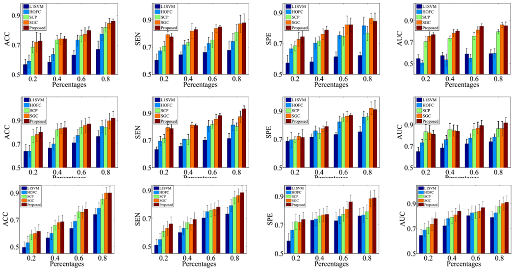
Classification results (mean ± standard deviation) of personalized classification on FTD (upper row), OCD (middle row), and ADNI (bottom row).
First, our method obtains the best performance at different settings, followed by SGC, SCP, HOFC, and L1SVM. For example, our method on average improves 3.55%, compared to the best comparison method SGC, in terms of all four evaluation metrics, on three data sets with 80% labelled subjects for the training process. Moreover, the performance of supervised learning methods (e.g., L1SVM, SCP, and HOFC) in Fig. 3 is worse than their performance in Table II since the former used less training information, compared to the latter.
Second, all methods received worse performance when the percentage of labelled subjects is small. The reason is that inefficient subjects cannot guarantee to construct significant classifiers. However, the improvement of our method over supervised learning methods (e.g., L1SVM, SCP, and HOFC) with small percentages of labelled subjects, i.e., 20%, is larger than its improvement with large percentages of labelled subjects, e.g., 80%, since the former case can use more information than the latter one. The same case can be found in the comparison between SGC and supervised learning methods. This demonstrates the advantages of unlabelled data for the training process again.
3). Fusion Effectiveness:
All methods first converted the matrix representation (i.e., either the fully-connected FCNs or the sparse FCNs) to the vector representation, which is further fed to traditional classifiers for disease diagnosis. The key novelty of our proposed method is the parameter-free multi-band fusion model using multi-band information. Hence, we fed the sparse FCNs produced by our method (with 80% labelled subjects and 20% unlabelled subjects for the training process) to the methods (e.g., L1SVM and SGC) to verify the effectiveness of our proposed fusion model. We did not apply our outputted FCNs to either HOFC or SCP due to their model limitations. We listed the results in Fig. 4.
Fig. 4.
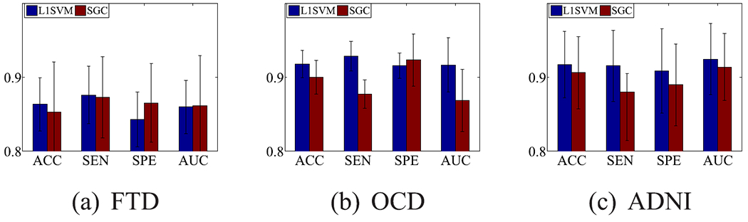
Classification results of the comparison methods using the FCNs outputted by our method.
The performance of both L1SVM and SGC in Fig. 4 are better than their performance in the case with 80% labelled subjects in Table II. For example, the result of SGC in Fig. 4 on average improves 0.88%, 3.53%, and 1.48%, compared to the results in Table II, in terms of accuracy on data sets FTD, OCD, and ADNI. The result of L1SVM in Fig. 4 on average improves 21.19%, 16.70%, and 18.33%, respectively, compared to the results in Table II, in terms of all four evaluation metrics on FTD, OCD, and ADNI. The reasons are (1) Fig. 4 used more information (i.e., 20% unlabelled subjects), compared to Table II for L1SVM; and (2) Fig. 4 used sparse FCNs, while Table II used fully-connected FCN. Furthermore, the performance of L1SVM in Fig. 4 is very similar to the performance of our method with 80% labelled data in Table II. The reason is that L1SVM using sparse FCNs produced by our method is exactly our proposed functional connectivity analysis framework.
4). Feature Selection Effectiveness:
In this section, we designed two kinds of experiments to investigate the effectiveness of the selected features by our method.
In our experiments, the 10-fold cross-validation scheme was utilized to evaluate the hyper-parameter C of the ℓ1-SVM method by setting the values of C as a list {2−6, 2−5, …, 26}. Each fold reported the best value of the hyper-parameter C and the corresponding selected features by the ℓ1-SVM, which resulted in 10 sets of selected features after the 10-fold cross-validation scheme. These selected features were the most important features in each fold. We repeated these 10-fold cross-validation scheme 10 times with different random seeds and collected all the 100 sets of selected features. The frequencies of the features presented in the 100 sets were then summarized. We selected the features that appeared at least 90 times as the final set of selected features. Since the features input in the ℓ1-SVM were the coefficients of correlation between two brain regions, each selected feature had two corresponding brain regions. We summarized the frequencies of the presents of these brain regions in the final set of selected features. Finally, the top 10 brain regions were reported and visualized in our paper. As a result, our method selected 980, 593, and 702 out of 4005 nodes, respectively, on the data sets FTD, OCD, and ADNI, while L1SVM selected 1357, 922, and 970 nodes, respectively. In our experiments, we first applied the selected nodes from our method to L1SVM and SGC for disease diagnosis, and then plotted top selected brain regions selected by L1SVM and our method. We reported the results in Fig. 5.
Fig. 5.
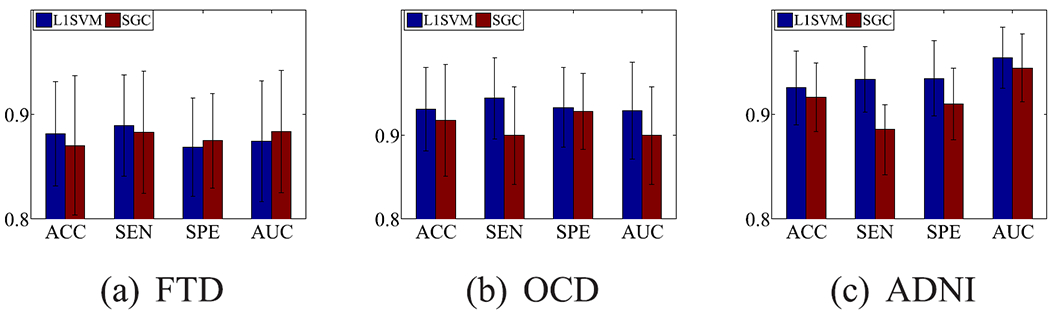
Classification results of L1SVM and SGC using the features selected by our method.
The performance of both L1SVM and SGC in Fig. 5 is better than their performance in Fig. 4 because the former used a part of the features (i.e., 980, 593, and 702 out of 4005 nodes, for FTD, OCD, and ADNI, respectively) while the latter used all 4005 features. This implies the effectiveness of feature selection in our method. Furthermore, L1SVM used the features selected by our method means that our method conducts the ℓ1-SVM twice. For example, the second feature selection only uses 1357 features, which was selected by the first feature selection from all 4005 features on FTD. This demonstrates that high-dimensional data may degrade the model performance due to the issue of the curse of dimensionality.
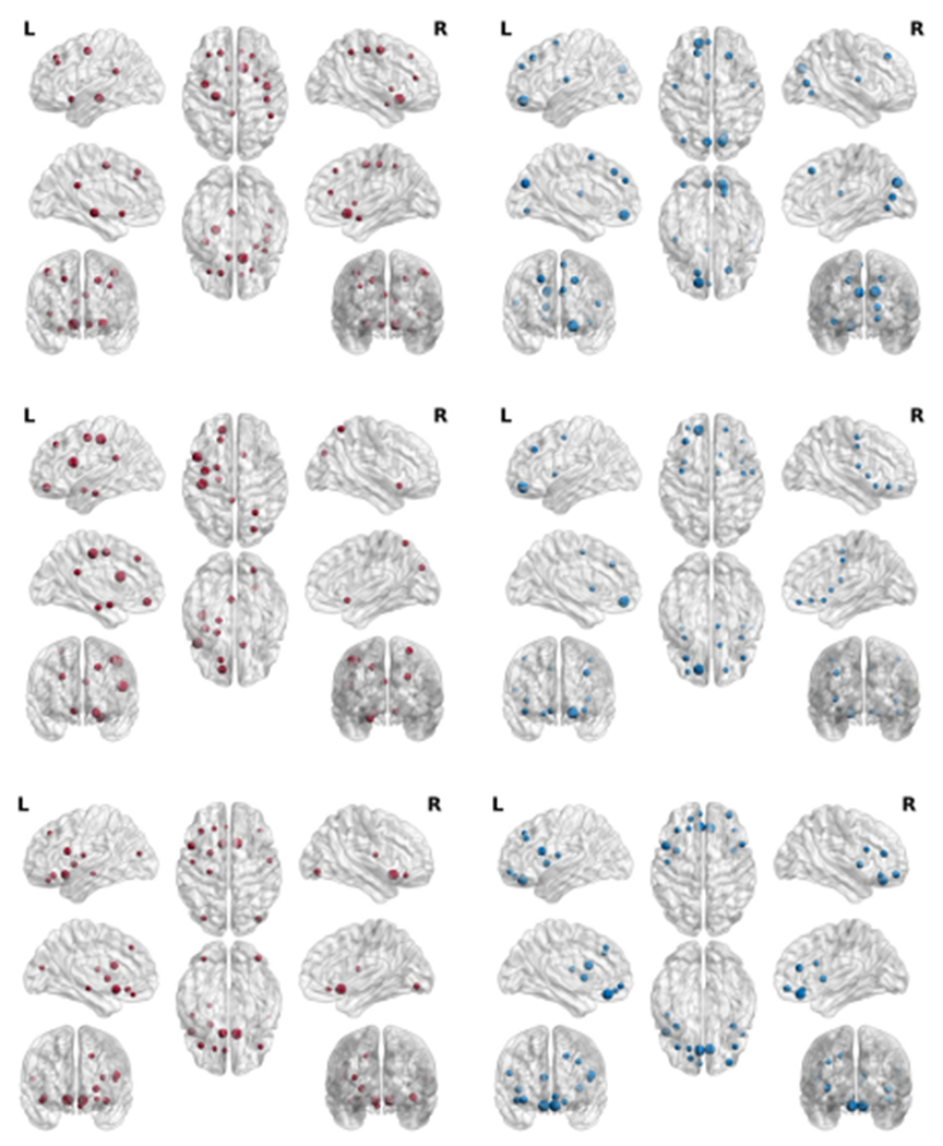
Based on the visualization of the top selected brain regions, many selected regions from both L1SVM and our method have been verified to be related to the neuro-diseases. Moreover, the number of selected brain regions associated with the neuro-disease with our method is larger than the number selected by L1SVM. This implies that our method is effective for both feature selection and disease diagnosis. Specifically, first, in Fig. 6, most of the nodes selected by our method occur in the frontal and temporal lobes, which is consistent with the current neurobiological findings on FTD ([44]). However, a large portion of nodes identified by L1SVM located at the occipital lobe and posterior parietal lobe, which are less relevant to FTD ([44]). Second, our method finds the brain regions, such as orbital-frontal cortex, caudate, thalamus, which are included in the cortical-striato-thalamic circuits, and is considered as the theoretical neuro-anatomical network of OCD ([45], [46]). Third, Alzheimer’s disease is associated with whole brain atrophy [47], our method selected the brain regions throughout the whole brain while L1SVM only selected the frontal regions on the data set ADNI.
Fig. 6.
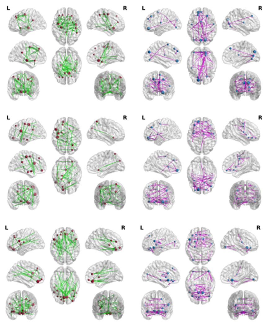
Visualization of top selected brain regions selected and the connected regions by L1SVM (left column) and our method (right column) on FTD (top row), OCD (middle row), and ADNI (bottom row).
IV. Discussion
In this section, we discuss the effectiveness of the multi-band signals, the variations of our proposed method with different k values, and the convergence analysis of our proposed Algorithm 1, using our proposed method (with 80% labelled subjects and 20% unlabelled subjects for the training process) to conduct personalized classification.
A. Effectiveness of Multi-Band Signals
We utilized the following steps to obtain multi-band frequency signals. First, the signals’ length was padded into the nearest value of 2 powers, guaranteeing the non-destructive wavelet decomposition [48], [49]. Therefore, the signals’ length in the data sets FTD and OCD was padded to 256, and the signals’ length in the data set ADNI was padded to 128. To do this, we used the traditional zero-padding technique [50] to reduce the edge effect on the wavelet decomposition. Second, the Discrete Wavelet Transform (DWT) was performed on the padded signals to decompose them into multi-bands. In our experiments, we followed the traditional Mallat algorithm to decompose the signal into a subband tree [51], [52]. As a result, we controlled the depth of the subband tree to partition the signals with the frequency range from 0.01HZ to 0.08HZ into four different frequencies, i.e., [0.01, 0.01875], [0.01875, 0.0275], [0.0275, 0.045], and [0.045, 0.08], as shown in Table III. In this paper, we set experiments to investigate the effectiveness of multi-band signals and reported the experimental results of our proposed method in Fig. 8.
TABLE III.
The Details of Different Frequency Bands on Three Data Sets
| Band number (g) | FTD /OCD /ADNI |
|---|---|
| 2 | [0.01HZ, 0.045HZ], [0.045HZ, 0.08HZ] |
| 3 | [0.01HZ, 0.0275HZ], [0.0275HZ, 0.045HZ], [0.045HZ, 0.08HZ] |
| 4 | [0.01HZ, 0.01875HZ], [0.01875HZ, 0.0275HZ], [0.0275HZ, 0.045HZ], [0.045HZ, 0.08HZ] |
Fig. 8.
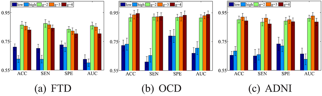
Classification results (mean ± standard deviation) of our proposed method with different frequency bands on three data sets, where “low” and “high”, respectively, indicate the single frequency band with the range as [0.01 HZ, 0.04HZ] and [0.04HZ, 0.08HZ]. In particular, “Proposed” is actually the case of g = 2.
Fig. 8 indicates the following conclusions. First, our proposed method with multi-band signals (i.e., g = 2/3/4) outperforms our method with the single frequency signals (i.e., “low” and “high”). This verifies that it is reasonable to take into account multi-band signals for the analysis of fMRI data. For example, the classification results with the setting g = 2 on the data set FTD on average improves 10.76% and 11.18%, compared to “low” and “high”. Second, different data sets require various multi-band signal decomposition. For example, the data set FTD achieved the best classification performance with g = 2. The data sets OCD and ADNI, respectively, achieved the best classification performance with g = 4 and g = 3. Third, with the increase of the decomposition times, the information of the signals in the low frequency bands is gradually diluted and the number of the frequency bands increases. In this manner, the fusion process is more challengeable, compared to the scenarios with fewer decomposition times. The effectiveness of the proposed method is thus affected. That is, there exists the optimal decomposition time.
Physiologically, the unsuitable decomposition time (e.g., large values of g in this work) may weaken the ability to disentangle the complex neural activity [53]. For example, [53] found that the signal decomposition with two to four decomposition times can differentiate normal and pathological brain regions.
B. Effectiveness of k Values
Fig. 9 reports the classification results of our proposed method with different k values on three data sets. Obviously, our proposed method is insensitive to the variations of k value as the difference of the classification results between two different values of k on three data sets is small. For example, our method achieved the best classification result with the k value of 10, 10, and 5, respectively, for the data sets FTD, OCD, and ADNI. These best classification results only averagely increase 2.48%, 0.79%, and 3.10%, respectively, compared to the worst results on the data sets FTD, OCD, and ADNI, in terms of all evaluation metrics.
Fig. 9.
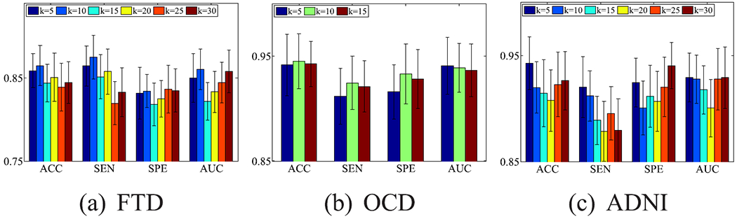
Classification results (mean ± standard deviation) of our proposed method with different values of k on three data sets.
C. Convergence Analysis
We experimentally analyze the convergence of Algorithm 1 in Fig. 10. Algorithm 1 monotonically decreases the objective function values in Eq. (5) until Algorithm 1 achieves convergence. Moreover, Algorithm 1 only needs around ten iterations to achieve the convergence. Hence, our proposed Algorithm 1 is efficient.
Fig. 10.
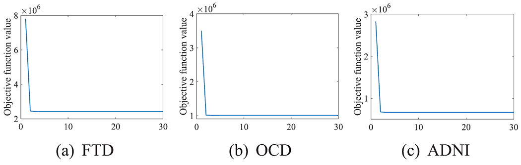
Convergence analysis of our proposed Algorithm 1 at different iterations on three data sets.
V. Conclusion
In this paper, we proposed a new multi-band fusion framework for personalized disease diagnosis, by two sequential steps, parameter-free multi-band fusion and joint brain region selection & disease diagnosis. Experimental results on three real-world data sets demonstrated the effectiveness of our proposed framework, compared to state-of-the-art methods. Moreover, experimental results also verified the effectiveness of each step in our proposed framework.
Based on our experiments and the literature, deep learning methods (such as SGC and DeepLight [18]) usually achieve high classification performance by learning robust deep features, but these obtained deep features lack interpretability. In our future work, we prefer to apply our proposed fusion framework in deep learning models to achieve good classification performance as well as interpretability.
Fig. 7.
Visualization of top selected brain regions selected by L1SVM (left column) and our method (right column) on FTD (top row), OCD (middle row), and ADNI (bottom row).
Acknowledgments
This work was supported in part by the National Key Research and Development Program of China under Grant 2018AAA0102200; in part by the National Natural Science Foundation of China under Grant 61876046; in part by the Guangxi “Bagui” Teams for Innovation and Research; in part by the Marsden Fund of New Zealand under Grant MAU1721; in part by the NIH under Grant AG049089, Grant AG068399, and Grant AG059065; and in part by the Sichuan Science and Technology Program under Grant 2018GZDZX0032 and Grant 2019YFG0535.
Footnotes
Contributor Information
Rongyao Hu, Center for Future Media, University of Electronic Science and Technology of China, Chengdu 611731, China; School of Computer Science and Technology, University of Electronic Science and Technology of China, Chengdu 611731, China; Massey University at Albany Campus, Auckland 0745, New Zealand.
Ziwen Peng, Guangdong Key Laboratory of Mental Health and Cognitive Science, Center for the Study of Applied Psychology, School of Psychology, South China Normal University, Guangzhou 510631, China.
Xiaofeng Zhu, Center for Future Media, University of Electronic Science and Technology of China, Chengdu 611731, China; School of Computer Science and Technology, University of Electronic Science and Technology of China, Chengdu 611731, China; Massey University at Albany Campus, Auckland 0745, New Zealand.
Jiangzhang Gan, Center for Future Media, University of Electronic Science and Technology of China, Chengdu 611731, China; School of Computer Science and Technology, University of Electronic Science and Technology of China, Chengdu 611731, China; Massey University at Albany Campus, Auckland 0745, New Zealand.
Yonghua Zhu, Center for Future Media, University of Electronic Science and Technology of China, Chengdu 611731, China; School of Computer Science and Technology, University of Electronic Science and Technology of China, Chengdu 611731, China; Massey University at Albany Campus, Auckland 0745, New Zealand.
Junbo Ma, School of Medicine, University of North Carolina at Chapel Hill, NC 27599 USA; Department of Computer Science, University of North Carolina at Chapel Hill, NC 27599 USA.
Guorong Wu, School of Medicine, University of North Carolina at Chapel Hill, NC 27599 USA; Department of Computer Science, University of North Carolina at Chapel Hill, NC 27599 USA.
References
- [1].Jie B, Liu M, and Shen D, “Integration of temporal and spatial properties of dynamic connectivity networks for automatic diagnosis of brain disease,” Med. Image Anal, vol. 47, pp. 81–94, Jul. 2018. [DOI] [PMC free article] [PubMed] [Google Scholar]
- [2].Guo Y, Gao Y, and Shen D, “Deformable MR prostate segmentation via deep feature learning and sparse patch matching,” IEEE Trans. Med. Imag, vol. 35, no. 4, pp. 1077–1089, Apr. 2016. [DOI] [PMC free article] [PubMed] [Google Scholar]
- [3].Hafkemeijer A et al. , “A longitudinal study on resting state functional connectivity in behavioral variant frontotemporal dementia and Alzheimer’s disease,” J. Alzheimer’s Disease, vol. 55, no. 2, pp. 521–537, Nov. 2016. [DOI] [PubMed] [Google Scholar]
- [4].Kong D, Ibrahim JG, Lee E, and Zhu H, “FLCRM: Functional linear cox regression model,” Biometrics, vol. 74, no. 1, pp. 109–117, Mar. 2018. [DOI] [PMC free article] [PubMed] [Google Scholar]
- [5].Shu H, Qu Z, and Zhu H, “D-GCCA: Decomposition-based generalized canonical correlation analysis for multiple high-dimensional datasets,” 2020, arXiv:2001.02856. https://arxiv.org/abs/2001.02856 [PMC free article] [PubMed] [Google Scholar]
- [6].Sahoo D, Satterthwaite TD, and Davatzikos C, “Extraction of hierarchical functional connectivity components in human brain using resting-state fMRI,” 2019, arXiv:1906.08365. [Online]. Available: http://arxiv.org/abs/1906.08365 [DOI] [PubMed] [Google Scholar]
- [7].Shu H, Wang X, and Zhu H, “D-CCA: A decomposition-based canonical correlation analysis for high-dimensional datasets,” J. Amer. Stat. Assoc, vol. 115, pp. 1–29, Jan. 2019. [DOI] [PMC free article] [PubMed] [Google Scholar]
- [8].Kong D, An B, Zhang J, and Zhu H, “L2RM: Low-rank linear regression models for high-dimensional matrix responses,” J. Amer. Stat. Assoc, pp. 1–7, Apr. 2019. [DOI] [PMC free article] [PubMed] [Google Scholar]
- [9].Zhang Y et al. , “Strength and similarity guided group-level brain functional network construction for MCI diagnosis,” Pattern Recognit., vol. 88, pp. 421–430, Apr. 2019. [DOI] [PMC free article] [PubMed] [Google Scholar]
- [10].Yang L et al. , “Gradual disturbances of the amplitude of low-frequency fluctuations (ALFF) and fractional ALFF in Alzheimer spectrum,” Frontiers Neurosci, vol. 12, p. 975, Dec. 2018. [DOI] [PMC free article] [PubMed] [Google Scholar]
- [11].Wang H et al. , “Functional brain connectivity revealed by sparse coding of large-scale local field potential dynamics,” Brain Topography, vol. 32, no. 2, pp. 255–270, Mar. 2019. [DOI] [PMC free article] [PubMed] [Google Scholar]
- [12].Gohel SR and Biswal BB, “Functional integration between brain regions at rest occurs in multiple-frequency bands,” Brain Connectivity, vol. 5, no. 1, pp. 23–34, Feb. 2015. [DOI] [PMC free article] [PubMed] [Google Scholar]
- [13].Wang J et al. , “Frequency-specific alterations of local synchronization in idiopathic generalized epilepsy,” Medicine, vol. 94, no. 32, p. e1374, 2015. [DOI] [PMC free article] [PubMed] [Google Scholar]
- [14].Hallquist MN, Hwang K, and Luna B, “The nuisance of nuisance regression: Spectral misspecification in a common approach to resting-state fMRI preprocessing reintroduces noise and obscures functional connectivity,” NeuroImage, vol. 82, pp. 208–225, Nov. 2013. [DOI] [PMC free article] [PubMed] [Google Scholar]
- [15].Kalthoff D, Seehafer JU, Po C, Wiedermann D, and Hoehn M, “Functional connectivity in the rat at 11.7T: Impact of physiological noise in resting state fMRI,” NeuroImage, vol. 54, no. 4, pp. 2828–2839, Feb. 2011. [DOI] [PubMed] [Google Scholar]
- [16].Fransson P, “Spontaneous low-frequency BOLD signal fluctuations: An fMRI investigation of the resting-state default mode of brain function hypothesis,” Hum. Brain Mapping, vol. 26, no. 1, pp. 15–29, 2005. [DOI] [PMC free article] [PubMed] [Google Scholar]
- [17].Lowe MJ, Mock BJ, and Sorenson JA, “Functional connectivity in single and multislice echoplanar imaging using resting-state fluctuations,” Neuroimage, vol. 7, no. 2, pp. 119–132, 1998. [DOI] [PubMed] [Google Scholar]
- [18].Thomas AW, Heekeren HR, Müller K-R, and Samek W, “Analyzing neuroimaging data through recurrent deep learning models,” Frontiers Neurosci, vol. 13, pp. 13–21, Dec. 2019. [DOI] [PMC free article] [PubMed] [Google Scholar]
- [19].Thompson GJ, Pan W-J, and Keilholz SD, “Different dynamic resting state fMRI patterns are linked to different frequencies of neural activity,” J. Neurophysiol, vol. 114, no. 1, pp. 114–124, Jul. 2015. [DOI] [PMC free article] [PubMed] [Google Scholar]
- [20].Whitwell JL and Josephs KA, “Recent advances in the imaging of frontotemporal dementia,” Current Neurol. Neurosci. Rep, vol. 12, no. 6, pp. 715–723, Dec. 2012. [DOI] [PMC free article] [PubMed] [Google Scholar]
- [21].Reyes P et al. , “Functional connectivity changes in behavioral, semantic, and nonfluent variants of frontotemporal dementia,” Behavioural Neurol, vol. 2018, pp. 1–10, Apr. 2018. [DOI] [PMC free article] [PubMed] [Google Scholar]
- [22].Eavani H, Satterthwaite TD, Filipovych R, Gur RE, Gur RC, and Davatzikos C, “Identifying sparse connectivity patterns in the brain using resting-state fMRI,” NeuroImage, vol. 105, pp. 286–299, Jan. 2015. [DOI] [PMC free article] [PubMed] [Google Scholar]
- [23].Hinrich JL, Bardenfleth SE, Røge RE, Churchill NW, Madsen KH, and Mørup M, “Archetypal analysis for modeling multisubject fMRI data,” IEEE J. Sel. Topics Signal Process, vol. 10, no. 7, pp. 1160–1171, Oct. 2016. [Google Scholar]
- [24].Zhang Y et al. , “Hierarchical feature fusion framework for frequency recognition in SSVEP-based BCIs,” Neural Netw, vol. 119, pp. 1–9, Nov. 2019. [DOI] [PubMed] [Google Scholar]
- [25].Chen JE and Glover GH, “BOLD fractional contribution to resting-state functional connectivity above 0.1 Hz,” NeuroImage, vol. 107, pp. 207–218, Feb. 2015. [DOI] [PMC free article] [PubMed] [Google Scholar]
- [26].Weinberger KQ and Saul LK, “Distance metric learning for large margin nearest neighbor classification,” J. Mach. Learn. Res, vol. 10, no. 2, pp. 207–244, Feb. 2009. [Google Scholar]
- [27].Li H, Satterthwaite TD, and Fan Y, “Large-scale sparse functional networks from resting state fMRI,” NeuroImage, vol. 156, pp. 1–13, Aug. 2017. [DOI] [PMC free article] [PubMed] [Google Scholar]
- [28].Fan R-E, Chang K-W, Hsieh C-J, Wang X-R, and Lin C-J, “LIBLINEAR: A library for large linear classification,” J. Mach. Learn. Res, vol. 9, no. 8, pp. 1871–1874, Jun. 2008. [Google Scholar]
- [29].Daubechies I, DeVore R, Fornasier M, and Güntürk CS, “Iteratively reweighted least squares minimization for sparse recovery,” Commun. Pure Appl. Math, vol. 63, no. 1, pp. 1–38, 2010. [Google Scholar]
- [30].Boyd S, “Convex optimization of graph Laplacian eigenvalues,” in Proc. ICM, pp. 1311–1319, vol. 3, nos. 1–3, 2006. [Google Scholar]
- [31].Duchi J, Shalev-Shwartz S, Singer Y, and Chandra T, “Efficient projections onto the l1-ball for learning in high dimensions,” in Proc. 25th Int. Conf. Mach. Learn. (ICML), 2008, pp. 272–279. [Google Scholar]
- [32].Zhou Y, Zhang L, Teng S, Qiao L, and Shen D, “Improving sparsity and modularity of high-order functional connectivity networks for MCI and ASD identification,” Frontiers Neurosci, vol. 12, pp. 959–970, Dec. 2018. [DOI] [PMC free article] [PubMed] [Google Scholar]
- [33].Zille P, Calhoun VD, Stephen JM, Wilson TW, and Wang Y-P, “Fused estimation of sparse connectivity patterns from rest fMRI—Application to comparison of children and adult brains,” IEEE Trans. Med. Imag, vol. 37, no. 10, pp. 2165–2175, Oct. 2018. [DOI] [PMC free article] [PubMed] [Google Scholar]
- [34].Zhu X, Zhang S, Zhu Y, Zhu P, and Gao Y, “Unsupervised spectral feature selection with dynamic hyper-graph learning,” IEEE Trans. Knowl. Data Eng, early access, Aug. 18, 2020, doi: 10.1109/TKDE.2020.3017250. [DOI] [Google Scholar]
- [35].Shen HT, Zhu Y, Zheng W, and Zhu X, “Half-quadratic minimization for unsupervised feature selection on incomplete data,” IEEE Trans. Neural Netw. Learn. Syst, vol. 32, no. 7, pp. 3122–3135, Jul. 2020, doi: 10.1109/TNNLS.2020.3009632. [DOI] [PubMed] [Google Scholar]
- [36].Dong C et al. , “Impairment in the goal-directed corticostriatal learning system as a biomarker for obsessive–compulsive disorder,” Psychol. Med, vol. 59, no. 9, pp. 1490–1500, 2019. [DOI] [PubMed] [Google Scholar]
- [37].Zang YF et al. , “Altered baseline brain activity in children with ADHD revealed by resting-state functional MRI,” Brain Develop, vol. 29, no. 2, pp. 83–91, 2007. [DOI] [PubMed] [Google Scholar]
- [38].Byrge L and Kennedy DP, “Identifying and characterizing systematic temporally-lagged BOLD artifacts,” NeuroImage, vol. 171, pp. 376–392, May 2018. [DOI] [PMC free article] [PubMed] [Google Scholar]
- [39].Lankinen K et al. , “Consistency and similarity of MEG- and fMRI-signal time courses during movie viewing,” NeuroImage, vol. 173, pp. 361–369, Jun. 2018. [DOI] [PubMed] [Google Scholar]
- [40].Tzourio-Mazoyer N et al. , “Automated anatomical labeling of activations in SPM using a macroscopic anatomical parcellation of the MNI MRI single-subject brain,” NeuroImage, vol. 15, no. 1, pp. 273–289, 2002. [DOI] [PubMed] [Google Scholar]
- [41].Zhang H, Chen X, Zhang Y, and Shen D, “Test-retest reliability of ‘high-order’ functional connectivity in young healthy adults,” Frontiers Neurosci, vol. 11, pp. 439–458, Aug. 2017. [DOI] [PMC free article] [PubMed] [Google Scholar]
- [42].Wu F, Souza A, Zhang T, Fifty C, Yu T, and Weinberger K, “Simplifying graph convolutional networks,” in Proc. ICML, 2019, pp. 6861–6871. [Google Scholar]
- [43].Nair V and Hinton G, “Rectified linear units improve restricted Boltzmann machines,” in Proc. 27th Int. Conf. Mach. Learn. (ICML), 2010, pp. 807–814. [Google Scholar]
- [44].de Haan W et al. , “Functional neural network analysis in frontotemporal dementia and Alzheimer’s disease using EEG and graph theory,” BMC Neurosci, vol. 10, no. 1, pp. 101–112, Dec. 2009. [DOI] [PMC free article] [PubMed] [Google Scholar]
- [45].Gillan CM et al. , “Disruption in the balance between goal-directed behavior and habit learning in obsessive-compulsive disorder,” Amer. J. Psychiatry, vol. 168, no. 7, pp. 718–726, Jul. 2011. [DOI] [PMC free article] [PubMed] [Google Scholar]
- [46].Gillan CM et al. , “Functional neuroimaging of avoidance habits in obsessive-compulsive disorder,” Amer. J. Psychiatry, vol. 172, no. 3, pp. 284–293, Mar. 2015. [DOI] [PMC free article] [PubMed] [Google Scholar]
- [47].Schott JM, Crutch SJ, Frost C, Warrington EK, Rossor MN, and Fox NC, “Neuropsychological correlates of whole brain atrophy in Alzheimer’s disease,” Neuropsychologia, vol. 46, no. 6, pp. 1732–1737, May 2008. [DOI] [PubMed] [Google Scholar]
- [48].Gogolewski D, “Influence of the edge effect on the wavelet analysis process,” Measurement, vol. 152, Feb. 2020, Art. no. 107314. [Google Scholar]
- [49].Zhang Z, Wang Y, and Wang K, “Fault diagnosis and prognosis using wavelet packet decomposition, Fourier transform and artificial neural network,” J. Intell. Manuf, vol. 24, no. 6, pp. 1213–1227, Dec. 2013. [Google Scholar]
- [50].Montanari L, Basu B, Spagnoli A, and Broderick BM, “A padding method to reduce edge effects for enhanced damage identification using wavelet analysis,” Mech. Syst. Signal Process, vols. 52–53, pp. 264–277, Feb. 2015. [Google Scholar]
- [51].Malekian V, Nasiraei-Moghaddam A, Akhavan A, and Hossein-Zadeh G-A, “Efficient de-noising of high-resolution fMRI using local and sub-band information,” J. Neurosci. Methods, vol. 331, Feb. 2020, Art. no. 108497. [DOI] [PubMed] [Google Scholar]
- [52].Zeng W, Li M, Yuan C, Wang Q, Liu F, and Wang Y, “Identification of epileptic seizures in EEG signals using time-scale decomposition (ITD), discrete wavelet transform (DWT), phase space reconstruction (PSR) and neural networks,” Artif. Intell. Rev, vol. 53, no. 4, pp. 3059–3088, Apr. 2020. [Google Scholar]
- [53].Saritha M, Joseph KP, and Mathew AT, “Classification of MRI brain images using combined wavelet entropy based spider web plots and probabilistic neural network,” Pattern Recognit. Lett, vol. 34, no. 16, pp. 2151–2156, Dec. 2013. [Google Scholar]