

Abstract
Cortical thickness varies throughout the cortex in a systematic way. However, it is challenging to investigate the patterns of cortical thickness due to the intricate geometry of the cortex. The cortex has a folded nature both in radial and tangential directions which forms not only gyri and sulci but also tangential folds and intersections. In this article, cortical curvature and depth are used to characterize the spatial distribution of the cortical thickness with much higher resolution than conventional regional atlases. To do this, a computational pipeline was developed that is capable of calculating a variety of quantitative measures such as surface area, cortical thickness, curvature (mean curvature, Gaussian curvature, shape index, intrinsic curvature index, and folding index), and sulcal depth. By analyzing 501 neurotypical adult human subjects from the ABIDE‐I dataset, we show that cortex has a very organized structure and cortical thickness is strongly correlated with local shape. Our results indicate that cortical thickness consistently increases along the gyral–sulcal spectrum from concave to convex shape, encompassing the saddle shape along the way. Additionally, tangential folds influence cortical thickness in a similar way as gyral and sulcal folds; outer folds are consistently thicker than inner.
Keywords: cortical folding, cortical thickness, curvature, gyrus, shape index, sulcus
Cortical thickness varies throughout the cortex in a systematic way. In this article, we developed an open‐source computational pipeline that is capable of calculating a variety of quantitative surface measures, to characterize the spatial distribution of the cortical thickness. By analyzing 501 neurotypical adult human subjects from the ABIDE‐I dataset, we show that cortex has a very organized structure and cortical thickness is strongly correlated with local shape.

1. INTRODUCTION
Each human brain has a unique structure and morphology, similar to fingerprints. The outermost layer of the brain, the cerebral cortex, has many intricate convolutions consisting of outer ridges called gyri and inner valleys called sulci. The cortex is fairly smooth until the third trimester of gestation, when these folds begin to emerge. Importantly, while gyral and sulcal folds are the subject of most research, the cortex folds not only in the radial direction (forming gyri and sulci), but also in the tangential direction. Visible on the surface of the brain (Figure 1), gyri and sulci fold in on themselves and even intersect (Chen et al., 2017; Razavi, Liu, & Wang, 2021; Razavi, Zhang, Li, Liu, & Wang, 2015; Zhang et al., 2017; Zhang et al., 2018).
FIGURE 1.

Folds of the human brain. Left: Coronal section of a T1‐weighted magnetic resonance (MR) image for a human subject showing gyral tops, sulcal valleys and sulcal walls in a two‐dimensional slice. Right: Tangential folds shown in black splines on the three‐dimensional surface of the brain
The thickness of the cortex throughout the convolutions of the brain is important because cortical thickness is a biomarker of neurological health. Alterations of cortical thickness are observed in atypical development (Vijayakumar et al., 2016), preterm birth (Nam et al., 2015), and neurological diseases such as autism spectrum disorder (ASD) (Ecker et al., 2010; Ecker et al., 2013; Hardan, Muddasani, Vemulapalli, Keshavan, & Minshew, 2006; Misaki, Wallace, Dankner, Martin, & Bandettini, 2012; Pua, Ball, Adamson, Bowden, & Seal, 2019; van Rooij, Anagnostou, & Arango, 2018; Zielinski et al., 2014), schizophrenia (van Erp et al., 2018; White, Andreasen, Nopoulos, & Magnotta, 2003), and attention deficit hyperactivity disorder (ADHD) (Montes et al., 2013; Narr et al., 2010). Cortical thinning is also observed in the prefrontal cortex of typical adults during normal aging (Salat et al., 2004) and in Alzheimer's disease (Lerch & Evans, 2005).
Cortical thickness is not uniform throughout the brain, with a striking asymmetry between thick gyri and thin sulci (Bok, 1929; Campos, Hornung, Gompper, Elgeti, & Caspers, 2020; Holland et al., 2020; Holland, Budday, Goriely, & Kuhl, 2018; Jalil Razavi, Zhang, Liu, & Wang, 2015; Razavi et al., 2015) (Van Essen & Maunsell, 1980). This intriguing property of the cortex has been consistently demonstrated among humans (Fatterpekar et al., 2002; Fischl & Dale, 2000; Ge et al., 2018; Ribas, 2010; Zhang et al., 2016) and various species (Hilgetag & Barbas, 2005; Welker, 1990). The complete rationale behind this thickness difference is yet to be elucidated, but given the relevance of cortical thickness to neurological health, these variations, and their determinants are important fundamental and clinical questions. It is important to consider cortical thickness not as a global property of an entire brain, but rather a local, spatially varying property. For instance, thinning in Alzheimer's disease is systematically nonuniform, with sulci thinning and degenerating more than gyri (Lin et al., 2021).
Although the mechanism of cortical folding is still under investigation, a combination of mechanical and biological factors is thought to affect the buckling of the cortical sheet (Borrell, 2018; Garcia, Kroenke, & Bayly, 2018; Kroenke & Bayly, 2018). Recently, the formation of thick gyri and thin sulci has been the subject of research in an attempt to understand how this pattern emerges so consistently.
Advances in numerical simulations have allowed increasingly complex simulations of brain development (Bayly, Okamoto, Xu, Shi, & Taber, 2013; Nie et al., 2010; Tallinen, Chung, Biggins, & Mahadevan, 2014; Toro & Burnod, 2005). The interactions between the faster tangential growth of the cortex in comparison with the underlying white matter core, supplemented by the cerebrospinal fluid (CSF) pressure (Van Essen, 2020), lead to buckling of the surface (Caviness, 1975). Tensional forces along axons and glia resist the detachment of cortex from the core and likely bring strongly connected gyri closer to each other (Van Essen, 2020). We recently showed that wrinkling instabilities and the buckling of the cortex lead to thick gyri and thin sulci without any influence from biological heterogeneity (Holland et al., 2018).
However, local changes in cellular growth and development likely also contribute to the thickness variations seen in the brain. During growth, the newly born cells in the ventricular zone migrate toward their final destinations in the outer regions to form layers of the cortex which consist of distinctive neuronal cell populations (Cowan, 1979). The neuronal cell bodies in gyral crowns are more spread out, with dense and elaborately branched neuropils (axons, dendrites, glial cells, and their synapses) stretching vertically to the cortical surface. On the other hand, cell bodies and their basal dendrites in sulcal fundi are more densely packed and stretch tangential to the cortical surface (Cowan, 1979; Welker, 1990). These particular trajectories suggest tension within these cellular processes that contributes to cortical thickness variations and affects the macroscopic mechanical properties of the brain in vivo (Van Essen, 1997).
In our most recent work, we introduced a curvature‐dependent mechanical growth model capable of modeling different growth rates in gyri and sulci. By comparing the gyral–sulcal thickness ratio in our simulations with data from human brains, we found evidence for preferential gyral growth in the cortex (Wang, Demirci, & Holland, 2020). This result is consistent with previous knowledge that more neurons are present in gyri compared to sulci banks and bottoms (Hilgetag & Barbas, 2005) causing thicker gyral crests.
However, as mentioned previously, the cortex features not only gyral peaks and sulcal valleys, but also in‐plane bends and intersections of gyri and sulci (Figure 1). This suggests that the traditional binary classification of cortical folding into gyri and sulci, while able to capture a lot of the variation seen in 2D histological slices, may be insufficient to represent the full three‐dimensional complexity of the brain. If forces generated during folding contribute to thickness differences throughout the cortex, it seems possible that these folds could affect thickness as well. This would imply that cortical folds exist along a gyral–sulcal spectrum, with the outside of tangentially folded gyri at one end, and the inside of tangentially folded sulci at the other. Cortical thickness variations in the tangential folds of gyri and sulci have been explored in a few studies (Chen et al., 2013; Chen et al., 2017; Ge et al., 2018; Li, Lin, & Gilmore, 2015; Zhang et al., 2017; Zhang et al., 2018), but these analyses have been limited to a few dozen regions defined by brain atlases. Brain atlases automatically parcellate the cortex into functional or anatomical regions (Desikan et al., 2006; Destrieux, Fischl, Dale, & Halgren, 2010) by relying on cortical shape and widely accepted anatomical descriptions. The Destrieux atlas (Destrieux et al., 2010), for example, segments the cortex into predominately gyral and sulcal regions. Regional studies of cortical thickness (Holland et al., 2018; Zhang et al., 2016) show consistent cortical thickness variations between regions, but they are limited. First of all, automatically extracting and labeling the regions of a cortex using a predefined anatomical atlas (reference template) is a challenging task, requiring complex surface‐based (Fischl, Sereno, Tootell, & Dale, 2001) and/or landmark‐based (Van Essen, Glasser, Dierker, Harwell, & Coalson, 2012) diffeomorphic spherical registration algorithms that align cortical folding patterns with the reference template. However, this approach generates local distortions and transformations within the gyral–sulcal patterns which consequently causes deviations from the original, native space, although “gentler” multimodal algorithms are suggested (Robinson et al., 2014). Secondly, this classification is binary, which results in straight sulcal walls being identified as sulci. Furthermore, it is not possible to cleanly divide every gyrus from its adjacent sulci, and vice versa, so some regions are a combination of both. Finally, the averaging of cortical thickness across the region discards a significant amount of information about variations within the region. These limitations highlight the importance of quantifying cortical morphology on smaller scales (Dahnke & Gaser, 2018; Mangin, Jouvent, & Cachia, 2010) and in native space in order to fully capture variations throughout the brain.
Automated computational neuroimaging software has proven to be very useful for the segmentation, reconstruction, and analysis of 3D brain morphology from 2D magnetic resonance (MR) image slices. Widely used software packages in the field include Freesurfer (Fischl, 2012), Mindboggle (Klein et al., 2017), CAT (Gaser & Dahnke, 2016), toolbox of SPM (Ashburner, 2009), Brains2 (Magnotta et al., 2002), CIVET (Kabani, Le Goualher, MacDonald, & Evans, 2001), and BrainVisa (Cointepas, Mangin, Garnero, Poline, & Benali, 2001), as well as Connectome Workbench for visualization of neuroimaging data (Marcus et al., 2011). Although these software packages are very powerful and have proven extremely useful in neuroimaging research, they have generally been focused on adult human brains, offering even highly automated segmentation and analysis. While there are some efforts to develop automatic processing pipelines for infants (Zöllei, Iglesias, Ou, Grant, & Fischl, 2020) and non‐human primates (Klink, 2020), those are still under development. Furthermore, the automation of these pipelines, while a strength in many senses, can also be a drawback; for instance, it is often not possible to customize the mesh resolution or smoothness. Finally, these programs report but do not focus on curvature, which is of primary interest in this study; to the best of our knowledge, for instance, none of the software packages mentioned above calculate shape index. The website https://www.nitrc.org provides a comprehensive list of frequently used neuroimaging tools and software packages that are useful for various neuroimaging tasks.
In this study, we aim to investigate the folded morphology of the brain, including both radial and tangential folds, and the variation of cortical thickness along the gyral–sulcal spectrum. By investigating how the cortical thickness varies across the convoluted surface of the brain beyond gyri and sulci, we expect to observe thickness variations within the tangential folds as well. To do so, we analyzed cortical thickness on a local scale, without following an automated parcellation scheme. We employed three curvature measures (mean curvature, Gaussian curvature, and shape index), along with sulcal depth, to demonstrate the systematic cortical thickness variations of the cortex with respect to local cortical topology. While these curvature measures have been investigated in the brain before (Batchelor et al., 2002; Cachia et al., 2001; Hu, Chen, Hung, Guo, & Wu, 2013; Koenderink & van Doorn, 1992; Luders et al., 2006; Pienaar, Fischl, Caviness, Makris, & Grant, 2008; Ronan et al., 2011; Ronan et al., 2014; Shimony et al., 2016; Tosun et al., 2007), this is, to the best of our knowledge, the first comprehensive local study of cortical thickness variations with respect to local shape.
To fulfill this aim, and to overcome the challenges of already available automated neuroimaging software packages, we developed our own in‐house, open‐source computational pipeline that allows for detailed local analysis of cortical thickness and topology. This pipeline is introduced in Section 2, and is shared publicly via https://github.com/mholla/curveball. Next, in Section 3 we present the systematic and consistent variation of cortical thickness with respect to local curvature and depth for a sample subject set. Finally, in Section 4, we consider how each measure of topology (mean curvature, Gaussian curvature, shape index, and sulcal depth) reveals features of the cortex's complex folded surface.
2. METHODS
Our analysis begins with the inner and outer surfaces of the cortical sheet (white and pial surfaces, respectively) reconstructed from cross‐sectional MR images. While our pipeline can take any set of surface meshes as an input, here we used Freesurfer (Dale, Fischl, & Sereno, 1999; Fischl, 2012), which outputs a piecewise triangular mesh for both surfaces with ~150 k vertices per hemisphere. Both meshes are decimated and smoothed to improve uniformity (Section 2.1), and the cortical thickness is calculated at each vertex (Section 2.2). Next, an outer alpha‐wrap surface is generated from the pial surface to obtain the sulcal depth at each point (Section 2.3). The pipeline then computes the Gaussian curvature (Section 2.4.1), mean curvature (Section 2.4.2), principal curvatures (Section 2.4.3), shape index (Section 2.4.4), total intrinsic curvature index (ICI), and total folding index (FI) (Section 2.4.5). Finally, all surface data are smoothed with two iterations of averaging with neighbors (Section 2.5). The total run‐time of the pipeline is approximately 1.5 hr per hemisphere using a single‐core processor.
2.1. Mesh decimation and smoothing
The accuracy of quantitative surface measures depends on the quality of the mesh. As surface reconstruction from MR images introduces noise, a more uniform, simplified, and smoothed mesh is necessary to reduce the irregularities of the original mesh (Dahnke & Gaser, 2018) and improve the signal‐to‐noise ratio. To achieve this, we used quadratic edge collapse decimation with a target reduction value of 70% and Laplacian and Taubin smoothing (Ohtake, Belyaev, & Bogaevski, 2001; Sorkine, 2005; Taubin, 1995) algorithms (Cignoni et al., 2008) (Figure 2a,b). In a previous study, 70% down‐sampling of Freesurfer‐generated pial surfaces yielded an error value below 0.2 mm for both gyri and sulci (Tran & Fang, 2017). This decimation results in approximately 40 k vertices and 80 k triangles per hemisphere. Laplacian and Taubin smoothing are applied for 50 and 100 iterations, respectively. These values were found to avoid over‐smoothing and shrinkage of the surface while preserving the original topology (Figure 3). Less convoluted areas are covered with slightly fewer triangles and vice versa. To assess the quality of the decimated mesh, we compared the radius ratio and aspect ratio of its triangular elements before and after mesh decimation and smoothing using open‐source 3D mesh processing software Meshlab (Cignoni et al., 2008). Radius ratio (Tecchio & Basso, 2014) is the ratio of the radii of the circle inscribed in a triangle, , and the triangle’s circumsphere, ; it is calculated for triangle as
| (1) |
where a is the total area of the triangle and , , and are its edge lengths. Radius ratio ranges from 0 to 1, with an optimal value of 1 for an equilateral triangle. Aspect ratio is the ratio of a triangle’s area to its longest edge length, with low values indicating stretched‐out obtuse triangles. After decimation, we observed 15% improvement in the radius and aspect ratios (Figure 4), particularly by eliminating many of the most distorted triangles.
FIGURE 2.

Decimation and smoothing of triangular surface meshes of the pial (a) and white (b) surfaces. The left column shows an irregular mesh with ~150 k vertices and ~300 k triangles per hemisphere. The right column shows a simplified, uniform mesh with ~40 k vertices and ~80 k triangles per hemisphere
FIGURE 3.

Cortical surface mesh smoothing. Left: Original surface mesh after reconstruction. Middle: After 50 iterations of Laplacian smoothing. Right: After 100 iterations of Taubin smoothing
FIGURE 4.

Improvement of the surface triangular mesh shown by a histogram. Left: Radius ratio, or the ratio between r in (the radius of the triangle's inscribed circle) and r circ (the radius of the triangle's circumsphere). Right: Aspect ratio, where a is the total area of triangle and l is the longest edge length. The lighter plot corresponds to the original surface mesh, while the darker plot corresponds to the mesh after decimation and smoothing. The red shaded areas represent highly distorted elements. Figure generated by (Cignoni et al., 2008)
2.2. Cortical thickness
Accurate estimation of the cortical thickness through automated segmentation of pial and white surfaces is important for understanding the inhomogeneous development of the cortex and hidden columnar boundaries (MacDonald, Kabani, Avis, & Evans, 2000). Freesurfer generates white and pial surface meshes with identical numbers of vertices, and calculates the cortical thickness as the average of the distances from the point on the white surface to its nearest neighbor on the pial surface, and from the point on the pial surface to its nearest neighbor on the white surface (Fischl & Dale, 2000). This method has been shown to be reliable by comparing the results with manual measurements from MR (Kuperberg et al., 2003) and histological slices (Cardinale et al., 2014; Rosas et al., 2002). Other methods to calculate the cortical thickness (Wagstyl & Lerch, 2018) include Laplace's equation (Jones, Buchbinder, & Aharon, 2000), the shortest distance along the surface normal (MacDonald et al., 2000), the distance between linked vertices on the pial and white surfaces (MacDonald et al., 2000), and the shortest distance to the nearest vertex (MacDonald et al., 2000). Here, we calculated the cortical thickness using the average method similar to Freesurfer, as it has been shown to yield the lowest standard deviation and lower normalized standard deviation values across repeated single subject and population scans (Lerch & Evans, 2005). Cortical thickness values outside the range of 1.6 and 4 mm might be assumed artifactual (Glasser et al., 2016; Glasser, Goyal, Preuss, Raichle, & Van Essen, 2014); to be more conservative, we used the limits of 0.5 and 5 mm, but our analyses are robust for either range. Limiting the cortical thickness to between 0.5 and 5 mm excludes approximately 2% of the vertices per hemisphere.
2.3. Sulcal depth
Sulcal shape descriptors, such as sulcal depth (Li et al., 2014), sulcal width (Jin, Zhang, Shaw, Sachdev, & Cherbuin, 2018; Madan, 2019), and the location and spatial frequency of sulcal pits (the deepest points of cortical sulci) (Im & Grant, 2019; Meng et al., 2018; Meng, Li, Lin, Gilmore, & Shen, 2014), have been investigated previously in order to explore cortical development (Im et al., 2010). Here, we focus on sulcal depth as an indicator of whether a point is toward the outer surface of the brain or deep in its interior. In general, sulcal distance is measured either relative to a morphological closing surface which tightly shrink‐wraps the cortical surface (Kao et al., 2007), or a mid‐surface that crosses the cortical surface (Fischl, Sereno, & Dale, 1999). Here, we incorporated both methods for our sulcal depth calculations (Figure 5). First, a point cloud is generated from the reconstructed pial surface mesh. Secondly, a morphological closing is achieved by generating an alpha surface which wraps the point cloud. Alpha shapes are generalizations of convex hulls, which wrap point clouds to varying degrees of tightness (Edelsbrunner, Kirkpatrick, & Seidel, 1983; Edelsbrunner & Mucke, 1994). The value of the arbitrary real parameter characterizes the shape of the point cloud; values close to zero capture the fine details of the set of points, while higher values create a convex hull (Gardiner, Behnsen, & Brassey, 2018). An alpha value of 20 yielded a plausible surface for closure of the cortex as it captured the shape of the outer cortical surface without extending into the sulcal valleys, while also outlining the concave medial temporal lobe and inferior medial regions (Figure 5 inset). After aligning both surfaces to a common origin, we shrink the alpha surface by a constant offset value at each node to generate a midcortical surface that divides the pial and white surfaces. The offset parameter was chosen to be 7 mm such that, in all subjects, roughly half of the vertices are outside the midcortical surface and half are inside. While a single parameter is not able to achieve a perfect fit for all subjects, this resulted in only a 5% difference between the number of inside and outside vertices in most of the subjects, with up to a 10% difference in ~10% of subjects. Finally, we calculate the Euclidean distance between each vertex on the cortical surface and the nearest vertex on the alpha surface. This is the sulcal depth, defined such that points buried in the brain's folds have a positive sulcal depth and points on the outer surface of the brain have a negative sulcal depth (Im et al., 2008; Van Essen, 2005). This method is different from the Freesurfer's sulcal depth measurement, which measures how far a vertex moves during an inflation operation (Fischl et al., 1999). Other depth measurement methods involve calculations of the shortest geodesic distance (Rettmann, Han, Xu, & Prince, 2002; Tosun et al., 2007) or the adaptive distance, which is a combination of both Euclidean and geodesic distances (Kao et al., 2007; Yun, Im, Yang, Yoon, & Lee, 2013). However, Euclidean and adaptive distance calculations perform similarly in distinguishing between control groups and Alzheimer patients (Yun et al., 2013), so for the sake of simplicity, we employ Euclidean distance.
FIGURE 5.

Generation of alpha surface for the calculation of sulcal depth. First, the 3D surface meshes reconstructed from the MR images using Freesurfer are smoothed and decimated. Secondly, the alpha surface is generated from the point cloud of the pial surface mesh (inset image shows the effect of alpha parameter). Finally, the outer alpha surface is isometrically shrunken to generate a midcortical surface
2.4. Curvature
The complex morphology of the cortex can be investigated by the characteristic shape of its convolutions via curvature measures (Batchelor et al., 2002; Hu et al., 2013; Pienaar et al., 2008; Shimony et al., 2016). In general, curvature is a scalar quantity that gives the amount of bending at a point on a convoluted surface. While there are many different ways to quantify curvature, only two are independent (Gray, 1998; Mesmoudi, De Floriani, & Magillo, 2012; Upadhyay, 2015). Here, we consider mean curvature, a measure of extrinsic curvature or folding; Gaussian curvature, a measure of intrinsic curvature or distortion; and shape index, a non‐dimensional indication of shape. Furthermore, we calculate the principal curvatures from the mean and Gaussian curvatures.
2.4.1. Gaussian curvature
Gaussian curvature is a surface invariant, or intrinsic property of a surface (Chiek, 2006). It does not change unless the surface is distorted, sheared, or stretched. It has previously been used to quantify degree of cortical folding and cortico‐cortical connection lengths (Ronan et al., 2011; Ronan et al., 2014). For discrete meshes, assuming that curvature is constant around a local neighborhood, Gaussian curvature at a given point can be calculated by the principles of Gauss‐Bonnet theorem (Gray, 1998; Surazhsky, Magid, Soldea, Elber, & Rivlin, 2003) by
| (2) |
where is the number of triangles connected to the vertex , is the internal angle of the ith triangle, and , , and are the triangle edge lengths as can be seen in Figure 6. is the sum of the area of each triangle , where is the semi perimeter of each triangle meeting at a vertex (Lin & Perry, 1982). It can also be written as , where is the sum of the internal angles at the point. If the local surface at a vertex is flat, then the sum of the internal angles would be and the Gaussian curvature is zero. However, if the surface is elliptic or hyperbolic, the sum of the internal angles will be less than or more than , respectively. On these surfaces, geodesic distances also change. Geodesics are the curves that minimize the lengths between two points on a curved surface (Hubbard, 2016); on a flat surface, the Euclidean and geodesic distances are equal (Hunsaker, 1941). A given area has a smaller geodesic radius when Gaussian curvature is negative than when it is positive.
FIGURE 6.

Representative polyhedra of the surface mesh at vertex p with N = 5 neighboring vertices. Edge l i is associated with internal angle θ i and dihedral angle β i (note that vertex p is not necessarily co‐planar with the neighboring vertices v i )
2.4.2. Mean curvature
Unlike Gaussian curvature, mean curvature is an extrinsic property of the surface, providing a useful measure of foldedness. It has an intuitive meaning, changing as a piece of paper is folded into a cone or cylinder. Just like paper folding, the extent of shape change might be restricted by intrinsic properties of the surface, such as its initial thickness and surface area (Mota & Herculano‐Houzel, 2015). The direction of the outward unit normal provides the orientation at a given point, so that the mean curvature distinguished between convex and concave shapes. It has previously been shown to be a good indicator of gyral and sulcal patterns of the cortex (Batchelor et al., 2002; Cachia et al., 2001; Luders et al., 2006). For discrete surfaces, the mean curvature can be calculated by
| (3) |
where is the number of edges connected to the vertex; denotes the length of the ith edge connected to the vertex ; is the dihedral angle, or the angle between normal vectors of the adjacent triangles meeting at the edge ; and is the sum of the areas of the adjacent triangles (Mesmoudi et al., 2012) (Figure 6). This formulation assumes that the neighboring vertices of the polygon is a cylindrical arc with a small radius tangent to adjacent edges.
2.4.3. Principal curvatures
At a given point on a curved surface, there are two orthogonal planes that correspond to the maximum and minimum normal curvatures, and , respectively. (Here we use the convention , but note that some studies instead use .) The principal curvatures are quantified as the reciprocal of the radius of the circle of best fit tangent to the surface at that point. The local shape of a point on an arbitrary surface can be determined by principle curvatures (Figure 7). They can be calculated from the mean and Gaussian curvature as and ) (Gray, 1998) or conversely, the mean and Gaussian curvature can be written in terms of principal curvatures as and , respectively. In this study, we calculated the principal curvatures from the values of mean and Gaussian curvature at each vertex (Hu et al., 2013).
FIGURE 7.

A combination of principle curvatures yields different shapes at a point on a surface
2.4.4. Shape index
Shape index is a dimensionless and scale‐independent surface measure (Koenderink & van Doorn, 1992), unlike the mean and Gaussian curvature, which have units of mm−1 and mm−2, respectively. Shape index can be calculated from the mean and Gaussian curvatures or from the principal curvatures,
| (4) |
Shape index has a value between −1 and 1, classifying a continuous gradient of concave, saddle, and convex shapes.
Planar surfaces, where , have an indeterminate shape index value. The absolute value of the shape index identifies the distinct shape and the sign of it represents the orientation. While both mean and Gaussian curvature are necessary to identify the local shape of a surface (shape, sharpness of fold, and direction), shape index can be used efficiently for discriminating local surface shape details uniquely and intuitively (Dorai & Jain, 1997). In addition, shape index is a useful quantitative measure of brain folding during growth, due to its scale‐independent property which separates isometric growth (scaling) and shape change. Cortical growth and development is known to be non‐uniform and it is challenging to analyze curvature and shape change independently from size change (Pienaar et al., 2008). To investigate shape change only, it is ideal to use a dimensionless measure (Hu et al., 2013); for example, shape index (Koenderink & van Doorn, 1992) has been used to differentiate the local shape of the cortex in fetal brains (Hu et al., 2013). Other approaches for obtaining scale‐independent curvature measures include normalizing by the surface area and cerebral volume (Shimony et al., 2016) or employing a Gaussian‐filter approach (Pienaar et al., 2008).
2.4.5. Intrinsic curvature index and folding index
The total ICI and total FI are dimensionless measures that quantify the total intrinsic curvature and total extrinsic folding of the cortex,
| (5) |
respectively (Van Essen & Drury, 1997). They are both normalized by which is the total integrated curvature for a perfect sphere as introduced by the well‐known Gauss‐Bonnet theorem. Whether the cortex is more intrinsically curved or extrinsically folded attracted researchers previously. They have tried to quantify this by generating 2D flat mappings of the cortex (Drury et al., 1996; Van Essen & Drury, 1997). If the cortex is only purely folded, then a 2D flat map could be generated with no distortions. However, cortex is also intrinsically curved that hinders 2D flat mappings without local cuts or tears.
2.5. Surface data smoothing
Discrete surface measure calculations on piece‐wise linear shapes introduce local minimums and maximums. To remove these local extrema, we applied a weighted‐average smoothing algorithm, averaging the surface data on a vertex with the data of its immediate neighbors by
| (6) |
where is the value at the vertex in consideration, is the value at its ith neighbor, is the weight parameter, and is the Euclidean distance between the vertex and its neighbor. While geodesic distance would be more robust for highly convoluted surfaces like the cortex, for fine meshes the difference is likely negligible (Chung et al., 2005). We employed two iterations of smoothing at each vertex.
2.6. Data
In this study, we present our results based on the Autism Brain Imaging Data Exchange (ABIDE‐I) repository (Di Martino et al., 2014). Although MRI data acquisition parameters and types of scanners vary between sites (Table 1), all of the scans were acquired at 3 T. Detailed information regarding the functional and anatomical scan parameters of each site can be found on the website http://fcon_1000.projects.nitrc.org/indi/abide/abide_I.html and also in the supplementary information of Di Martino et al. (2014). We analyzed the structural MR images of neurotypical human subjects of both sexes, between 7 and 64 years old. While 573 subjects are available in the ABIDE‐I database, we excluded 72 subjects based on qualitative scan quality (Pardoe et al., 2016). All structural MR images were preprocessed with Freesurfer pipeline (Fischl, 2012) (version 6.0, http://surfer.nmr.mgh.harvard.edu) to obtain reconstructed white and pial cortical surface meshes, which can be accessed via the website http://preprocessed-connectomes-project.org/abide/ (Cameron et al., 2013). Further analysis is executed by our publicly available computational pipeline shared via https://github.com/mholla/curveball.
TABLE 1.
Autism Brain Imaging Data Exchange MRI data acquisition details for each site
| Site | Sample size | Voxel size (mm3) | Scan parameters | Scanner | |||
|---|---|---|---|---|---|---|---|
| TR (ms) | TE (ms) | TI (ms) | Flip angle (°) | ||||
| Caltech | 19 | 1 × 1 × 1 | 1,590.0 | 2.73 | 800 | 10 | STT |
| CMU | 12 | 1 × 1 × 1 | 1,870.0 | 2.48 | 1,100 | 8 | SV |
| KKI | 31 | 1 × 1 × 1 | 8.0 | 3.70 | 843 | 8 | PA |
| Leuven‐1 | 15 | 0.98 × 0.98 × 1.2 | 9.6 | 4.60 | 900 | 8 | PI |
| Leuven‐2 | 20 | 0.98 × 0.98 × 1.2 | 9.6 | 3.06 | 900 | 8 | PI |
| MaxMun | 32 | 1 × 1 × 1 | 1,800.0 | 3.06 | 900 | 9 | SV |
| NYU | 104 | 1.3 × 1 × 1.3 | 2,530.0 | 3.25 | 1,100 | 7 | SA |
| OHSU | 11 | 1 × 1 × 1 | 2,300.0 | 3.58 | 900 | 10 | STT |
| Olin | 13 | 1 × 1 × 1 | 2,500.0 | 2.74 | 900 | 8 | SA |
| Pitt | 26 | 1.1 × 1.1 × 1.1 | 2,100.0 | 3.93 | 1,000 | 7 | SA |
| SBL | 15 | 1 × 1 × 1 | 9.0 | 3.50 | 1,000 | 8 | PI |
| SDSU | 21 | 1 × 1 × 1 | 11.1 | 4.30 | 600 | 45 | GEM |
| Stanford | 12 | 0.86 × 1.5 × 0.86 | 8.4 | 1.80 | NA | 15 | GES |
| Trinity | 25 | 1 × 1 × 1 | 8.5 | 3.90 | 1,060 | 8 | SV |
| UCLA‐1 | 30 | 1 × 1 × 1.2 | 2,300.0 | 2.84 | 853 | 9 | STT |
| UCLA‐2 | 11 | 1 × 1 × 1.2 | 2,300.0 | 2.84 | 853 | 9 | STT |
| UM‐1 | 37 | 2 × 2 × 1.2 | 250.0 | 1.80 | 500 | 15 | GES |
| UM‐2 | 20 | 2 × 2 × 1.2 | 250.0 | 1.80 | 500 | 15 | GES |
| USM | 40 | 1 × 1 × 1.2 | 2,300.0 | 2.91 | 900 | 9 | STT |
| Yale | 7 | 1 × 1 × 1 | 1,230.0 | 1.73 | 624 | 9 | STT |
Notes: Sample size reflects the total number of subjects analyzed in this study, which in some cases is lower than the number of subjects scanned due to scan quality (Pardoe, Kucharsky Hiess, & Kuzniecky, 2016).
Abbreviations: GEM, GE MR750; GES: GE Signa; PA, Philips Achieva; PI, Philips Intera; SA, Siemens Allegra; STT, Siemens TrioTim; SV, Siemens Verio.
3. RESULTS
For each subject, we calculated the surface area, cortical thickness, sulcal depth, and curvature (mean curvature, Gaussian curvature, and shape index) at each vertex of the decimated mesh (~40 k vertices and ~80 k faces per hemisphere). In addition, we calculated the total curvature (ICI and FI) for the cortical surface of each subject. We present the surface data distributions as a function of probability density with a Gaussian kernel density estimation, where the estimator bandwidth employs the Scott's Rule (Heidenreich, Schindler, & Sperlich, 2013). The x‐axis shows the data values and the y‐axis can be interpreted as the probability for a value in the interval (i.e., bandwith) to occur.
Moreover, we investigated the cortical thickness distributions relative to each measure of curvature and depth with the intent to reproduce previous knowledge of gyral and sulcal thickness variations and gain a deeper understanding of the relationship between complex cortical folding patterns and thickness differences beyond just gyri and sulci. The distribution profiles represent aggregate data from each subject.
Before presenting our results, we wish to draw the reader's attention to the distinction between topology and anatomy. By topology, we refer to the objective, quantifiable local shape of the cortex, including convex, concave, and saddle shapes. By anatomy, we refer to the features of the brain as labeled by trained experts, including gyri, sulci, and walls, based on a combination of topology, location, and normalized atlases. While these concepts are loosely related—that is, gyri are mostly convex and most convex shapes are found on gyri—there are locations in the brain that represent every possible combination of topology and anatomy (Figure 8).
FIGURE 8.

Topology versus anatomy in the cortex. While topology and anatomy are loosely related, with gyri and convexity, sulci and concavity, and walls and saddle shapes often found together, every possible combination of the two can be found in the brain. Here we visualize convex gyri, saddle‐shaped gyral bends, and local concavities located on gyral crowns; similarly (while harder to visualize), most sulci are concave, but saddle and convex shapes can also be found on sulci
In addition to calculating statistical significance via Welch's t‐test for unequal variances, we also calculated Cohen's d value, or effect size (Cohen, 1977), to quantify the differences between cortical thickness distributions in relationship to shape and depth. The effect size is the amount of difference between the compared data; note that it is independent of the sample size and better at quantifying the substantial differences and overlap between data. A large effect size is “grossly perceptible” (Cohen, 1977), while a medium effect size () is visible to the naked eye. A small effect size () might not be obvious, but should not necessarily be interpreted as a negligible difference. Effect sizes are only reported when the data compared are significantly different ().
3.1. Average cortical thickness
The average cortical thickness of the human cortex is around 2.5–3 mm and varies non‐uniformly from 0.5 to 4.5 mm throughout the cortex (Fischl & Dale, 2000), providing information about its underlying cytoarchitecture (Goulas et al., 2016). Across all the subjects, we found an average cortical thickness of 2.71 ± 0.8 mm (Figure 9), slightly higher than the reported averages of 2.44 ± 0.10 mm (Van Essen et al., 2012) and 2.6 (Glasser et al., 2016).
FIGURE 9.

Cortical thickness. Left: Regional mean and local cortical thickness are overlaid onto pial and artificially inflated surfaces of a representative left hemisphere. Right: Cortical thickness distribution of N = 501 typically developed human subjects (mean = 2.71 ± 0.8 mm)
3.2. Mean curvature
After calculating the mean curvature across the surface of the brain (Figure 10a), we saw that the visible gyral peaks had mostly negative curvature (convex shape), while the buried sulci had positive curvature (concave). However, while mean curvature is useful to distinguish convex from concave shapes, this binary discrimination is insufficient to analyze the true topology of the cortex. It is not the case that negative and positive mean curvature strictly denote gyri and sulci, respectively, although this has been used previously as a heuristic (Lin et al., 2021). Both gyri and sulci have vertices with both positive and negative mean curvature (Figures 8 and 10a). Saddle shapes of the cortex cannot be distinguished with mean curvature. When looking at the distribution of cortical thickness in convex and concave points, we found that points with negative mean curvature are significantly thicker than the points with positive mean curvature (2.88 and 2.47 mm, respectively, with ) (Figure 10c). Mean curvature has a medium effect on cortical thickness () (Figure 10d).
FIGURE 10.
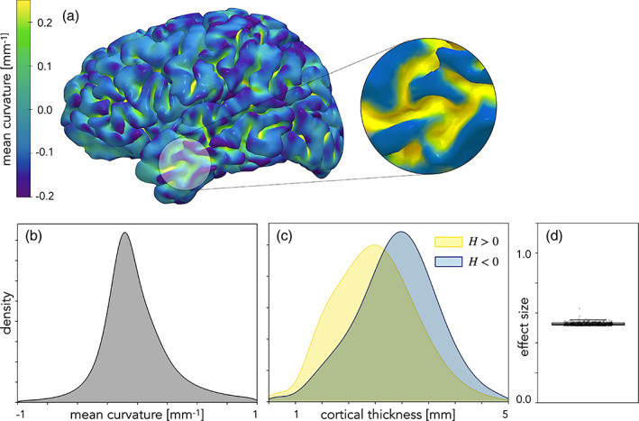
Mean curvature and cortical thickness. (a) Mean curvature is overlaid on the pial surface of a representative left hemisphere. The magnified image on the right shows the vertices with positive (yellow) and negative (blue) mean curvature. (b) Unimodal distribution of mean curvature for all N = 501 human subjects (mean ). Note that the range of mean curvature is restricted to [−1,1] to eliminate the outliers in the data. (c) Cortical thickness distribution for points with positive and negative mean curvature (H) with means 2.47 and 2.88 mm, respectively. (d) Effect size calculated for each subject (mean d = 0.53). The dotted lines show the cut‐off for large () and small () effect size thresholds
3.3. Gaussian curvature
When overlaying Gaussian curvature on the pial surface of the brain (Figure 11a), we saw that negative Gaussian curvature highlights the saddle‐shaped insides of tangential bends and intersections, while positive Gaussian curvature is found in both inward‐ and outward‐bulging areas. Thus, Gaussian curvature by itself is not able to distinguish between sulci and gyri. Instead, we supplemented Gaussian curvature with the principal curvatures. When both and are greater than zero, this indicates an inward‐bulging vertex, and vice versa. The mean value of the Gaussian curvature of inward‐bulging points and outward‐bulging points are 0.12 and 0.08 mm−2 for all subjects, respectively, as sulcal pits are more sharply folded than gyral peaks. The spatial frequency of vertices with saddle shape (~20 k vertices) are greater than convex (~12 k) or concave (~7 k) which might be evidence for the compact morphology of the cortex. The cortical thickness is thicker in convex points than concave points (2.96 and 2.33 mm, respectively), with saddle‐shaped vertices in between (2.70 mm) (Figure 11c). The distribution of cortical thickness is significantly different between the three shapes ( for all combinations), with a large effect size between concave and convex shapes and medium effect sizes between saddle shapes and the others (Figure 11d).
FIGURE 11.

Gaussian curvature and cortical thickness. (a) Gaussian curvature is overlaid onto the pial surface of a representative left hemisphere. The magnified image on the right shows the points with negative (yellow) and positive (blue) Gaussian curvature. (b) Unimodal distribution of Gaussian curvature for all human subjects . c) Cortical thickness distribution for convex , concave , and saddle‐shaped vertices with means 2.96 mm, 2.33 mm, and 2.70 mm respectively. d) Effect size calculated for each subject (means , respectively. The dotted lines show the cut‐off for large () and small () effect size thresholds
3.4. Shape index
From a qualitative assessment, shape index categorizes the cortical surface into a spectrum from the most inward‐folded areas, such as sulcal pits, to the most outward‐folded regions such as gyral crests (Figure 12a). In between are sulcal walls and the intersections and tangential folds of gyri and sulci, which exhibit various combinations of concavity and convexity. Unlike mean and Gaussian curvature, the distribution of the shape index throughout the cortex is bimodal with two distinct peaks (Figure 12b), corresponding to ridge and rut shapes (SI = −0.61 and 0.54). This means that most vertices are rut or ridge shaped, with ruts being the most prevalent. The distribution of cortical thickness with respect to the nine distinct shape descriptors of the shape index increases from cup to cap (Figure 12c). We comprehensively compared the thickness distribution for each shape to the others; every comparison was significant (). As expected, effect sizes are larger for more distinct shapes on opposite sides of the spectrum, and get smaller as the shape gets closer (Figure 12d).
FIGURE 12.

Shape index and cortical thickness. (a) Shape index is overlaid onto the pial surface of a representative left hemisphere. (b) Bimodal distribution of shape index for all N = 501 subjects, with peaks at −0.6 and 0.52. (c) Cortical thickness distribution for each descriptor of the shape index with means 2.34, 2.37, 2.39, 2.62, 2.74, 2.79, 2.86, 3.02, and 3.10 mm from cup to cap, respectively. (d) Effect size calculated for each combinations of the nine shape descriptors
3.5. Sulcal depth
After calculating sulcal depth from the hypothetical midcortical surface, the sulcal depth value is overlaid on the pial surface of the brain (Figure 13a). The midsurface cuts the pial surface in approximately two equal halves with respect to the total number of vertices in the outer and inner sections. Exterior points are significantly thicker than interior points (2.95 and 2.48 mm, respectively, with ), with a medium effect size (, Figure 13b,c).
FIGURE 13.

Sulcal depth and cortical thickness. (a) Sulcal depth is overlaid on the pial surface of a representative left hemisphere. Black dashed splines on the magnified images on the right show the midcortical surface with zero depth, both inside and outside of the tangential bends. (b) Cortical thickness distribution for the outer and inner halves of the pial surface for all N = 501 subjects. (c) Effect size calculated for each subject. The dotted lines show the cut‐off for large () and small () effect size thresholds
3.6. Interactions between curvature and depth
After investigating the distribution profile of cortical thickness in relationship to each curvature measure, we also considered interactions between curvature and depth (Figure 14). For each range of values, we calculated the mean cortical thickness of all the vertices within that range from all subjects. If no points in the desired range are found for a given subject (as occurs, e.g., when looking for sharply concave points in the outer reaches of the cortex), that subject is omitted from the calculations. For each shape, cortical thickness consistently increases when moving radially from the bottom of the sulci to the top of the gyri (Figure 14a–c). Additionally, for a given depth, convex shapes are thicker than concave shapes (as shown by mean curvature, Figure 14a, and shape index, Figure 14c), while saddle shapes are in between (as shown by Gaussian curvature, Figure 14b, and shape index, Figure 14c). Moreover, by observing the population size, we see that most convex points are in the exterior of the cortex, most concave points are in the interior, and saddle‐shaped vertices are clustered in the middle (sulcal walls).
FIGURE 14.

Cortical thickness variations with respect to curvature and depth. Average cortical thickness for all subjects with respect to a range of values of sulcal depth and (a) mean curvature, (b) Gaussian curvature, and (c) shape index. Note that cortical thickness is displayed as an averages for the given bounded values, weighted by the total number of vertices for each subject. The size of the circles indicate the number of points found in the bounded range. Insula is located deep in the cortex, >14 mm
Insula is the deepest region of the cortex, which has six gyral and sulcal subregions (shown in bright yellow color in Figure 13a). From a regional analysis of the insular cortex, we observed that its gyral regions have a higher mean cortical thickness value compared to its sulcal regions (ranging from 3.4 to 2.3 mm). From our local analysis, the correlation between shape and thickness is also evident for insula. Convex‐shaped points are thicker than concave‐shaped points in the insular region (Figure 14a–c) and saddle‐shaped points are in‐between these two (Figure 14b).
3.7. Intrinsic and extrinsic folding
We calculated the ICI and FI for all convex, concave, and saddle‐shaped points of the cortex as described in Section 2.4.5. They are normalized by their corresponding total surface area (~150 cm2 for concave, ~340 cm2 for convex, and ~590 cm2 for saddle). For saddle‐shaped points we took the absolute value of . Convex points are the least folded, while concave points are highly folded, with significantly higher and slightly higher . The saddle‐shaped points have a lower FI than concave points but similar curvature index (Figure 15).
FIGURE 15.

Normalized total ICI () and normalized total FI () for all convex, concave, and saddle‐shaped points of the cortex in N = 501 typically developed human subjects. Both folding indices are normalized by the total surface area of the relevant points
4. DISCUSSION
4.1. Cortical thickness varies along a gyral–sulcal spectrum
Cortical thickness variations in the cortex have been of great interest for decades, with early histological studies revealing a consistent difference in cytoarchitecture of the cortex where gyral crowns are thicker than sulcal fundi (Bok, 1929). However, these studies of two‐dimensional pieces of tissue could not capture the full complexity of the three‐dimensional pattern of folds seen in the human brain. With the advances of MR imaging and computational neuroimaging tools, it is now possible to investigate the intricate morphology of the brain and its variations in cortical thickness in three dimensions. Curvature measures are very useful in this matter. Although there is no single curvature measure that can capture the complex morphology in fine detail, each of the curvature measures investigated in this study can be useful for quantifying different aspects of the form of the cortex. Our analysis shows that the cortical thickness does not differ only between sulci and gyri (Figure 10), but rather gradually from sulci to gyri in a spectrum with respect to shape (Figures 11, 12, and 14). Cap shapes, with the highest convexity in both directions, are the thickest, while cup shapes, with the highest concavity in both directions, are the thinnest. In between are saddle shapes, which exhibit a combination of convexity and concavity.
4.2. Tangential folds affect the cortical thickness
The tangential folds of the cortex have not received much attention before, perhaps due to difficulties of outlining tangentially folded regions. Here, we show the usefulness of Gaussian curvature in highlighting tangential folding patterns (Figure 11a). Negative Gaussian curvature indicates the saddle shapes of the cortex, which corresponds to sharp circumferential infolds of gyri and sulci. These infolds are thinner than the outside of tangential folds, as identified by positive Gaussian curvature (Figure 14b). This result is consistent with previous results that found that convex regions were thicker than concave at adjacent banks of the precentral gyrus (Zhang et al., 2017). Furthermore, these inner folds are consistently thicker than purely concave regions but thinner than purely convex regions (Figure 11c). Tangential folds of the cortex have a consistent impact on the local cortical thickness.
4.3. Shape index reveals consistent thickness variations in relationship to local topology
While mean curvature distinguishes concave from convex, and Gaussian curvature distinguishes saddle shapes, shape index is able to classify the local shape in a continuous spectrum from sulcal crests to gyral peaks (Figure 12a–c). It is possible to discern the thickness variations with respect to shape for a given depth of the cortex. Shape index most clearly identifies the contribution of both of the principal curvatures, allowing us to distinguish shapes where convexity and concavity dominate to different extents. As the shapes shift from purely concave, to mostly concave, to mostly convex, to purely convex, the cortex consistently thickens. This could be because the local thickness restricts the local shape (Mota & Herculano‐Houzel, 2015), or the shape could be an indication of the stress state generated during folding, which naturally leads to local thickening and thinning (Holland et al., 2018). Furthermore, the size‐independent property of the shape index is very useful when comparing cortices of different sizes, for instance from different species or for a single individual throughout development. For example, shape index was found to best discriminate between term and healthy preterm infants (Shimony et al., 2016) and revealed subtle cortical shape differences among patients with Parkinsonian syndromes (Tosun et al., 2007).
4.4. Insular cortex shows the same patterns of thickness
Insula is the deepest region in the cortex, folded deep within the lateral sulcus. It emerges early on during gyrification before being covered by the neocortex, forming the complete Sylvian fissure (Van Essen, 2020). It has in total six gyral and sulcal subregions (Destrieux et al., 2010). From a local investigation, convex points of the insula are thicker than concave points. This explains why the cortex thickens after thinning as sulcal depth increases (Figure 14)—even though the insula is the most interior part of the cortex, it contains both gyri and sulci and therefore both thick and thin regions.
4.5. Extrinsic folding index varies in a gyral–sulcal spectrum
The entire cortex can be represented with a 2D flat map with minimal distortions as the cortex is more folded during gyrification than intrinsically curved (Van Essen & Maunsell, 1980). This is seen, for instance, in our findings that Gaussian curvature has a normal distribution with the majority of vertices very close to zero. In comparisons of ICI and FI, a noticeable predominance of extrinsic folding is found (Van Essen & Drury, 1997), particularly for concave and saddle points. This supports previous findings that sulcal invaginations involve a considerable amount of folding during growth (Van Essen & Maunsell, 1980). In fact, we observe an inverse correlation between the FI and cortical thickness, where concave points have the most folding and thinnest cortex, and convex points have the least folding and thickest cortex. This suggests a strong relationship between extrinsic folding and cortical thickness.
Intrinsic curvature quantifies areal distortions and shear, perhaps caused by non‐uniform, differential growth of the cortex (Griffin, 1994; Ronan et al., 2011; Ronan et al., 2014), and accompanies reduced geodesic distances. Higher in sulci might be a consequence of reduced connection lengths (Ronan et al., 2011). Furthermore, we note that saddle‐shaped vertices dominate the cortex (~55% of the total surface area), predominantly on tangential folds. Hyperbolic surfaces such as these lead to reduced geodesic distances, essentially bringing points on the surface closer to each other (Griffin, 1994). This could help overcome the challenges of packing increased cortical surface area into the limited cranial volume (Fernández, Llinares‐Benadero, & Borrell, 2016; Zhang & Sejnowski, 2000) and efficiently connecting different brain regions via the compact cortical wiring principle (Ronan et al., 2011; Van Essen, 1997). Thus, these folds, found in increasing numbers in highly convoluted brains, potentially enhance cortico‐cortical connections and brain function (Im et al., 2008).
4.6. Local cortical thickness has potential for the study of neurodevelopmental disorders
Recent advances in MR imaging and computational algorithms have opened possibilities for the diagnosis of neurological diseases and disorders based on abnormalities in cortical morphology (Gautam & Sharma, 2020; Raghavendra, Acharya, & Adeli, 2019; Tosun et al., 2007). For example, multivariate parametric classifier approaches have shown success at characterizing ASD from medical images, involving various morphological parameters of the brain such as total brain volume, total cortical volume, cortical thickness (Pua et al., 2019; van Rooij et al., 2018), mean curvature (Awate, Win, Yushkevich, Schultz, & Gee, 2008), sulcal depth (Nordahl et al., 2007), local gyrification index (Ni, Lin, Chen, Tseng, & Gau, 2019), and surface area (Ecker et al., 2010; Hong, Valk, Di Martino, Milham, & Bernhard, 2018; Mensen et al., 2017; Pua et al., 2019). While these results are difficult to generalize due to the heterogeneity of the disorder, which is influenced by various cofactors such as age, IQ, gender, and severity, future work could develop these cortical features into biomarkers for the early diagnosis of ASD in a clinical environment (Pagnozzi, Conti, Calderoni, Fripp, & Rose, 2018). Recent advances in high‐resolution MR imaging (Wagstyl et al., 2018), in particular, show great potential for investigating the relationship between local shape and thickness on a laminar scale. This could not only provide insight into the relationship between curvature and laminar thickness, but also the role of cortical laminae in both typical and atypical development.
4.7. Limitations
While this study represents the first comprehensive and systematic relationship between local cortical thickness and topology throughout the cortex, there are a several limitations. First, the ABIDE MR imaging dataset was selected arbitrarily, and we did not consider any age or gender effects. Quality control due to participant motion can be an issue for the ABIDE dataset (Bezgin, Lewis, & Evans, 2018; Di Martino et al., 2014; Esteban et al., 2017). A qualitative assessment of the image quality was performed previously that rated ABIDE scans from 1 to 5, 1 indicating a low quality with high motion artifact and 5 indicating a high quality with low motion artifact (Pardoe et al., 2016). We excluded in total subjects from our results that received a rating of 3 or below. However, our results did not change considerably when all the subjects were included in the analysis. We also note the challenges of multisite studies, where images were collected on different scanners with different parameters (Table 1); however, we separately analyzed subjects from a single site (Yale) and found very similar results. Additionally, we used cortical surface meshes generated by Freesurfer, which is optimized to work with adult human brains. This restricts our ability to analyze fetal or non‐human animal brains. However, our pipeline is capable of working on any surface mesh, so analyses such as these are only limited by the segmentation process, which can be done using other automated processes (Klein et al., 2017) or even manually (Heuer et al., 2019). Furthermore, the 70% decimation of the mesh results in significantly fewer vertices than are found in the original surface reconstructions from Freesurfer. This decimation parameter is adjustable in our pipeline, but was chosen because mesh resolution and computation time are inversely correlated. Currently, the total computation time is ~1–2 hr for a single subject, run with a single core, but a denser mesh would increase the total computation time substantially. Finally, this article focuses on the consistent relationship between the topology of the cortex and its thickness, without investigating the mechanisms for this relationship. Previous studies have established a plausible role for the mechanics of folding in the emergence of cortical thickness variations (Holland et al., 2018), while also pointing to a contributing role for heterogeneous growth throughout cortical folds (Wang et al., 2020). This work builds on those findings by identifying a systematic relationship between cortical folding and thickness. We leave future mechanistic investigations into the causes of cortical thickness variations, particularly those associated with cortical folding, to future studies.
5. CONCLUSION
Our findings offer a new framework for interpreting local cortical thickness variations throughout the cortex in much higher resolution than previous studies of cortical thickness. The convoluted shape of the cortex turns out to exhibit a well‐organized relationship between shape and thickness. This relationship is not limited to only the bottoms of sulci and the tops of gyri, but also observed in a variety of shapes beyond and in‐between, including the inner and outer edges of tangential folds and intersections. Cortical thickness was found to be significantly correlated with the local shape among typically developed human subjects. Convex points are consistently thicker than saddle‐shaped points, which are in turn consistently thicker than concave points. The more convex a point is (such as a spherical cap), the thicker it tends to be, with a smooth decrease in average thickness for shapes that display more and more concavity (such as saddle and cup shapes). Our findings point to an important role for tangential folds of gyri and sulci into the determination of cortical thickness. A consistent thickness variation has also been observed within the layers of the cortex; the deeper layers (Layers V and VI) are thinner along the fundus of a sulcus and relatively thicker along the crest of a gyrus, while the reverse is recognized for superficial Layers I, II, and III. The middle layer (Layer IV), on the other hand, has a fairly constant thickness in all regions for both in humans (Bok, 1929) and in macaques (Van Essen & Maunsell, 1980). We aim to investigate the well‐organized relationship between curvature and thickness within the layers of the cortex in the future.
CONFLICT OF INTERESTS
The authors declare that they have no conflict of interest.
ACKNOWLEDGMENTS
MAH acknowledges support from the National Science Foundation under grant no. IIS‐1850102.
Demirci, N. , & Holland, M. A. (2022). Cortical thickness systematically varies with curvature and depth in healthy human brains. Human Brain Mapping, 43(6), 2064–2084. 10.1002/hbm.25776
Funding information National Science Foundation, Grant/Award Number: IIS‐1850102
DATA AVAILABILITY STATEMENT
The data used in the preparation of this article is obtained from the Autism Brain Imaging Data Exchange I (ABIDE I) repository which is an international neuroimaging data‐sharing initiative. The data was obtained from the website http://fcon_1000.projects.nitrc.org/indi/abide/abide_I.html. All further analyses and visualization were performed by our publicly available computational pipeline (https://github.com/mholla/curveball).
REFERENCES
- Ashburner, J. (2009). Computational anatomy with the SPM software. Magnetic Resonance Imaging, 27(8), 1163–1174. 10.1016/j.mri.2009.01.006 [DOI] [PubMed] [Google Scholar]
- Awate, S. P. , Win, L. , Yushkevich, P. , Schultz, R. T. , & Gee, J. C. (2008). 3D cerebral cortical morphometry in autism: Increased folding in children and adolescents in frontal, parietal, and temporal lobes. In Metaxas D., Axel L., Fichtinger G., & Székely G. (Eds.), Medical image computing and computer‐assisted intervention – MICCAI 2008. Lecture notes in computer science (pp. 559–567). Berlin, Heidelberg: Springer. [DOI] [PubMed] [Google Scholar]
- Batchelor, P. , Castellano Smith, A. , Hill, D. , Hawkes, D. , Cox, T. , & Dean, A. (2002). Measures of folding applied to the development of the human fetal brain. IEEE Transactions on Medical Imaging, 21(8), 953–965. 10.1109/TMI.2002.803108 [DOI] [PubMed] [Google Scholar]
- Bayly, P. V. , Okamoto, R. J. , Xu, G. , Shi, Y. , & Taber, L. A. (2013). A cortical folding model incorporating stress‐dependent growth explains gyral wavelengths and stress patterns in the developing brain. Physical Biology, 10(1), 016005. 10.1088/1478-3975/10/1/016005 [DOI] [PMC free article] [PubMed] [Google Scholar]
- Bezgin, G. , Lewis, J. D. , & Evans, A. C. (2018). Developmental changes of cortical white–gray contrast as predictors of autism diagnosis and severity. Translational Psychiatry, 8(1), 249. 10.1038/s41398-018-0296-2 [DOI] [PMC free article] [PubMed] [Google Scholar]
- Bok, S. T. (1929). Der Einfluß Der in Den Furchen Und Windungen Auftretenden Krümmungen Der Groß Shirnrinde Auf Die Rindenarchitektur .
- Borrell, V. (2018). How cells fold the cerebral cortex. The Journal of Neuroscience, 38(4), 776–783. 10.1523/JNEUROSCI.1106-17.2017 [DOI] [PMC free article] [PubMed] [Google Scholar]
- Cachia, A. , Mangin, J.‐F. , Rivière, D. , Boddaert, N. , Andrade, A. , Kherif, F. , … Régis, J. (2001). A mean curvature based primal sketch to study the cortical folding process from antenatal to adult brain. In Niessen W. J., Viergever M. A. R., Goos G., Hartmanis J., & van Leeuwen J. (Eds.), Medical image computing and computer‐assisted intervention – MICCAI 2001. Lecture notes in computer science (Vol. 2208, pp. 897–904). Berlin, Heidelberg: Springer Berlin Heidelberg. 10.1007/3-540-45468-3_107 [DOI] [Google Scholar]
- Cameron, C. , Yassine, B. , Carlton, C. , Francois, C. , Alan, E. , András, J. , … Pierre, B. (2013). The neuro bureau preprocessing initiative: Open sharing of preprocessed neuroimaging data and derivatives. Frontiers in Neuroinformatics, 7. 10.3389/conf.fninf.2013.09.00041 [DOI] [Google Scholar]
- Campos, L. , Hornung, D. C. R. , Gompper, G. , Elgeti, J. , & Caspers, S. (2020). The role of thickness inhomogeneities in hierarchical cortical folding. NeuroImage, 231, 117779. [DOI] [PubMed] [Google Scholar]
- Cardinale, F. , Chinnici, G. , Bramerio, M. , Mai, R. , Sartori, I. , Cossu, M. , … Ferrigno, G. (2014). Validation of FreeSurfer‐estimated brain cortical thickness: Comparison with histologic measurements. Neuroinformatics, 12(4), 535–542. 10.1007/s12021-014-9229-2 [DOI] [PubMed] [Google Scholar]
- Caviness, V. (1975). Mechanical model of brain convolutional development. Science, 189(4196), 18–21. 10.1126/science.1135626 [DOI] [PubMed] [Google Scholar]
- Chen, H. , Li, Y. , Ge, F. , Li, G. , Shen, D. , & Liu, T. (2017). Gyral net: A new representation of cortical folding organization. Medical Image Analysis, 42, 14–25. 10.1016/j.media.2017.07.001 [DOI] [PMC free article] [PubMed] [Google Scholar]
- Chen, H. , Zhang, T. , Guo, L. , Li, K. , Yu, X. , Li, L. , … Liu, T. (2013). Coevolution of Gyral folding and structural connection patterns in primate brains. Cerebral Cortex, 23(5), 1208–1217. 10.1093/cercor/bhs113 [DOI] [PMC free article] [PubMed] [Google Scholar]
- Chiek, V . (2006). Geodesic on Surfaces of Constant Gaussian Curvature, 60.
- Chung, M. K. , Robbins, S. M. , Dalton, K. M. , Davidson, R. J. , Alexander, A. L. , & Evans, A. C. (2005). Cortical thickness analysis in autism with heat kernel smoothing. NeuroImage, 25(4), 1256–1265. 10.1016/j.neuroimage.2004.12.052 [DOI] [PubMed] [Google Scholar]
- Cignoni, P. , Callieri, M. , Corsini, M. , Dellepiane, M. , Ganovelli, F. , & Ranzuglia, G. (2008). MeshLab: An open‐source mesh processing tool. Computing, 1, 129–136. [Google Scholar]
- Cohen, J. (1977). CHAPTER 2 – The t test for means. In Cohen J. (Ed.), Statistical power analysis for the behavioral sciences (pp. 19–74). Mahwah, NJ: Academic Press. 10.1016/B978-0-12-179060-8.50007-4 [DOI] [Google Scholar]
- Cointepas, Y. , Mangin, J.‐F. , Garnero, L. , Poline, J.‐B. , & Benali, H. (2001). BrainVISA: Software platform for visualization and analysis of multi‐modality brain data. NeuroImage, 13(6), 98. 10.1016/S1053-8119(01)91441-7 [DOI] [Google Scholar]
- Cowan, W. M. (1979). The development of the brain. Scientific American, 23. [PubMed]
- Dahnke, R. , & Gaser, C. (2018). Surface and shape analysis. In Spalletta G., Piras F., & Gili T. (Eds.), Brain morphometry (Vol. 136, pp. 51–73). New York, NY: Springer. 10.1007/978-1-4939-7647-8_4 [DOI] [Google Scholar]
- Dale, A. M. , Fischl, B. , & Sereno, M. I. (1999). Cortical surface‐based analysis. I. Segmentation and surface reconstruction. NeuroImage, 9(2), 179–194. 10.1006/nimg.1998.0395 [DOI] [PubMed] [Google Scholar]
- Desikan, R. S. , Ségonne, F. , Fischl, B. , Quinn, B. T. , Dickerson, B. C. , Blacker, D. , … Killiany, R. J. (2006). An automated labeling system for subdividing the human cerebral cortex on MRI scans into gyral based regions of interest. NeuroImage, 31(3), 968–980. 10.1016/j.neuroimage.2006.01.021 [DOI] [PubMed] [Google Scholar]
- Destrieux, C. , Fischl, B. , Dale, A. , & Halgren, E. (2010). Automatic parcellation of human cortical gyri and sulci using standard anatomical nomenclature. NeuroImage, 53(1), 1–15. 10.1016/j.neuroimage.2010.06.010 [DOI] [PMC free article] [PubMed] [Google Scholar]
- Di Martino, A. , Yan, C.‐G. , Li, Q. , Denio, E. , Castellanos, F. X. , Alaerts, K. , … Milham, M. P. (2014). The autism brain imaging data exchange: Towards a large‐scale evaluation of the intrinsic brain architecture in autism. Molecular Psychiatry, 19(6), 659–667. 10.1038/mp.2013.78 [DOI] [PMC free article] [PubMed] [Google Scholar]
- Dorai, C. , & Jain, A. K. (1997). COSMOS‐A representation scheme for 3D free‐form objects. IEEE Transactions on Pattern Analysis and Machine Intelligence, 19(10), 1115–1130. 10.1109/34.625113 [DOI] [Google Scholar]
- Drury, H. A. , Van Essen, D. C. , Anderson, C. H. , Lee, C. W. , Coogan, T. A. , & Lewis, J. W. (1996). Computerized mappings of the cerebral cortex: A multiresolution flattening method and a surface‐based coordinate system. Journal of Cognitive Neuroscience, 8(1), 1–28. 10.1162/jocn.1996.8.1.1 [DOI] [PubMed] [Google Scholar]
- Ecker, C. , Ginestet, C. , Feng, Y. , Johnston, P. , Lombardo, M. V. , Lai, M.‐C. , … MRC AIMS Consortium . (2013). Brain surface anatomy in adults with autism: The relationship between surface area, cortical thickness, and autistic symptoms. JAMA Psychiatry, 70(1), 59. 10.1001/jamapsychiatry.2013.265 [DOI] [PubMed] [Google Scholar]
- Ecker, C. , Marquand, A. , Mourao‐Miranda, J. , Johnston, P. , Daly, E. M. , Brammer, M. J. , … Murphy, D. G. M. (2010). Describing the brain in autism in five dimensions–magnetic resonance imaging‐assisted diagnosis of autism spectrum disorder using a multiparameter classification approach. Journal of Neuroscience, 30(32), 10612–10623. 10.1523/JNEUROSCI.5413-09.2010 [DOI] [PMC free article] [PubMed] [Google Scholar]
- Edelsbrunner, H. , Kirkpatrick, D. , & Seidel, R. (1983). On the shape of a set of points in the plane. IEEE Transactions on Information Theory, 29(4), 551–559. 10.1109/TIT.1983.1056714 [DOI] [Google Scholar]
- Edelsbrunner, H. , & Mucke, E. P. (1994). Three‐dimensional alpha shapes. ACM Transactions on Graphics, 13(1), 43–72. [Google Scholar]
- Esteban, O. , Birman, D. , Schaer, M. , Koyejo, O. O. , Poldrack, R. A. , & Gorgolewski, K. J. (2017). MRIQC: Advancing the automatic prediction of image quality in MRI from unseen sites. PLoS One, 12(9), e0184661. 10.1371/journal.pone.0184661 [DOI] [PMC free article] [PubMed] [Google Scholar]
- Fatterpekar, G. M. , Naidich, T. P. , Delman, B. N. , Aguinaldo, J. G. , Gultekin, S. H. , Sherwood, C. C. , … Fayad, Z. A. (2002). Cytoarchitecture of the human cerebral cortex: MR microscopy of excised specimens at 9.4 tesla. American Journal of Neuroradiology, 23, 1313–1321. [PMC free article] [PubMed] [Google Scholar]
- Fernández, V. , Llinares‐Benadero, C. , & Borrell, V. (2016). Cerebral cortex expansion and folding: What have we learned? The EMBO Journal, 35(10), 1021–1044. 10.15252/embj.201593701 [DOI] [PMC free article] [PubMed] [Google Scholar]
- Fischl, B. (2012). FreeSurfer. NeuroImage, 62(2), 774–781. 10.1016/j.neuroimage.2012.01.021 [DOI] [PMC free article] [PubMed] [Google Scholar]
- Fischl, B. , & Dale, A. M. (2000). Measuring the thickness of the human cerebral cortex from magnetic resonance images. Proceedings of the National Academy of Sciences, 97(20), 11050–11055. 10.1073/pnas.200033797 [DOI] [PMC free article] [PubMed] [Google Scholar]
- Fischl, B. , Sereno, M. I. , & Dale, A. M. (1999). Cortical surface‐based analysis. II: Inflation, flattening, and a surface‐based coordinate system. NeuroImage, 9(2), 195–207. 10.1006/nimg.1998.0396 [DOI] [PubMed] [Google Scholar]
- Fischl, B. , Sereno, M. I. , Tootell, R. , & Dale, A. (2001). High‐resolution intersubject averaging and a coordinate system for the cortical thickness. Human Brain Mapping, 8(4), 272–284. [DOI] [PMC free article] [PubMed] [Google Scholar]
- Garcia, K. E. , Kroenke, C. D. , & Bayly, P. V. (2018). Mechanics of cortical folding: stress, growth and stability. Philosophical Transactions of the Royal Society B: Biological Sciences, 373(1759). 10.1098/rstb.2017.0321. [DOI] [PMC free article] [PubMed] [Google Scholar]
- Gardiner, J. D. , Behnsen, J. , & Brassey, C. A. (2018). Alpha shapes: Determining 3D shape complexity across morphologically diverse structures. BMC Evolutionary Biology, 18(1), 184. 10.1186/s12862-018-1305-z [DOI] [PMC free article] [PubMed] [Google Scholar]
- Gaser, C. , & Dahnke, R. (2016). CAT – A Computational Anatomy Toolbox for the Analysis of Structural MRI Data, 1. [DOI] [PMC free article] [PubMed]
- Gautam, R. , & Sharma, M. (2020). Prevalence and diagnosis of neurological disorders using different deep learning techniques: A meta‐analysis. Journal of Medical Systems, 44(2), 49. 10.1007/s10916-019-1519-7 [DOI] [PubMed] [Google Scholar]
- Ge, F. , Chen, H. , Zhang, T. , Wang, X. , Yuan, L. , Hu, X. , Guo, L. , & Liu, T. (2018). A novel framework for analyzing cortical folding patterns based on sulcal baselines and gyral crestlines. 2018 IEEE 15th International Symposium on Biomedical Imaging (ISBI 2018). Washington, DC: IEEE, pp. 1043–1047.
- Glasser, M. F. , Goyal, M. S. , Preuss, T. M. , Raichle, M. E. , & Van Essen, D. C. (2014). Trends and properties of human cerebral cortex: Correlations with cortical myelin content. NeuroImage, 93, 165–175. 10.1016/j.neuroimage.2013.03.060 [DOI] [PMC free article] [PubMed] [Google Scholar]
- Glasser, M. F. , Smith, S. M. , Marcus, D. S. , Andersson, J. L. R. , Auerbach, E. J. , Behrens, T. E. J. , … Van Essen, D. C. (2016). The human connectome project’s neuroimaging approach. Nature Neuroscience, 19(9), 1175–1187. 10.1038/nn.4361 [DOI] [PMC free article] [PubMed] [Google Scholar]
- Goulas, A. , Werner, R. , Beul, S. F. , Säring, D. , Heuvel, M. V. D. , Triarhou, L. C. , & Hilgetag, C. C. (2016). Cytoarchitectonic similarity is a wiring principle of the human connectome. bioRxiv. 10.1101/068254 [DOI] [Google Scholar]
- Gray, A. (1998). Modern differential geometry of curves and surfaces with mathematica (p. 996). Florida, FL: Chapman & Hall. [Google Scholar]
- Griffin, L. D. (1994). The intrinsic geometry of the cerebral cortex. Journal of Theoretical Biology, 166(3), 261–273. 10.1006/jtbi.1994.1024 [DOI] [PubMed] [Google Scholar]
- Hardan, A. Y. , Muddasani, S. , Vemulapalli, M. , Keshavan, M. S. , & Minshew, N. J. (2006). An MRI study of increased cortical thickness in autism. The American Journal of Psychiatry, 3, 1290–1292. [DOI] [PMC free article] [PubMed] [Google Scholar]
- Heidenreich, N.‐B. , Schindler, A. , & Sperlich, S. (2013). Bandwidth selection for kernel density estimation: A review of fully automatic selectors. Advances in Statistical Analysis, 97(4), 403–433. 10.1007/s10182-013-0216-y [DOI] [Google Scholar]
- Heuer, K. , Gulban, O. F. , Bazin, P.‐L. , Osoianu, A. , Valabregue, R. , Santin, M. , … Toro, R. (2019). Evolution of neocortical folding: A phylogenetic comparative analysis of MRI from 34 primate species. Cortex, 118, 275–291. 10.1016/j.cortex.2019.04.011 [DOI] [PubMed] [Google Scholar]
- Hilgetag, C. C. , & Barbas, H. (2005). Developmental mechanics of the primate cerebral cortex. Anatomy and Embryology, 210(5), 411–417. 10.1007/s00429-005-0041-5 [DOI] [PubMed] [Google Scholar]
- Holland, M. , Budday, S. , Goriely, A. , & Kuhl, E. (2018). Symmetry breaking in wrinkling patterns: Gyri are universally thicker than sulci. Physical Review Letters, 121(22), 228002. 10.1103/PhysRevLett.121.228002 [DOI] [PubMed] [Google Scholar]
- Holland, M. A. , Budday, S. , Li, G. , Shen, D. , Goriely, A. , & Kuhl, E. (2020). Folding drives cortical thickness variations. The European Physical Journal Special Topics, 229(17), 2757–2778. 10.1140/epjst/e2020-000001-6 [DOI] [PMC free article] [PubMed] [Google Scholar]
- Hong, S.‐J. , Valk, S. L. , Di Martino, A. , Milham, M. P. , & Bernhardt, B. C. (2018). Multidimensional neuroanatomical subtyping of autism spectrum disorder. Cerebral Cortex, 28(10), 3578–3588. 10.1093/cercor/bhx229 [DOI] [PMC free article] [PubMed] [Google Scholar]
- Hu, H.‐H. , Chen, H.‐Y. , Hung, C.‐I. , Guo, W.‐Y. , & Wu, Y.‐T. (2013). Shape and curvedness analysis of brain morphology using human fetal magnetic resonance images in utero. Brain Structure and Function, 218(6), 1451–1462. 10.1007/s00429-012-0469-3 [DOI] [PubMed] [Google Scholar]
- Hubbard, J. H. (2016). Teichmüller theory and applications to geometry, topology, and dynamics. Vol. 2. Surface homeomorphisms and rational functions . Matrix Editions, 262 pages, 108 color illustrations.
- Hunsaker, N. C. (1941). Hadamard’s theory op geodesics on surfaces op negative curvature. 38.
- Im, K. , & Grant, P. E. (2019). Sulcal pits and patterns in developing human brains. NeuroImage, 185, 881–890. 10.1016/j.neuroimage.2018.03.057 [DOI] [PMC free article] [PubMed] [Google Scholar]
- Im, K. , Jo, H. J. , Mangin, J.‐F. , Evans, A. C. , Kim, S. I. , & Lee, J.‐M. (2010). Spatial distribution of deep sulcal landmarks and hemispherical asymmetry on the cortical surface. Cerebral Cortex, 20(3), 602–611. 10.1093/cercor/bhp127 [DOI] [PubMed] [Google Scholar]
- Im, K. , Lee, J.‐M. , Lyttelton, O. , Kim, S. H. , Evans, A. C. , & Kim, S. I. (2008). Brain size and cortical structure in the adult human brain. Cerebral Cortex, 18(9), 2181–2191. 10.1093/cercor/bhm244 [DOI] [PubMed] [Google Scholar]
- Jalil Razavi, M. , Zhang, T. , Liu, T. , & Wang, X. (2015). Cortical folding pattern and its consistency induced by biological growth. Scientific Reports, 5(1), 14477. 10.1038/srep14477 [DOI] [PMC free article] [PubMed] [Google Scholar]
- Jin, K. , Zhang, T. , Shaw, M. , Sachdev, P. , & Cherbuin, N. (2018). Relationship between sulcal characteristics and brain aging. Frontiers in Aging Neuroscience, 10, 339. 10.3389/fnagi.2018.00339 [DOI] [PMC free article] [PubMed] [Google Scholar]
- Jones, S. E. , Buchbinder, B. R. , & Aharon, I. (2000). Three‐dimensional mapping of cortical thickness using Laplace's equation. Human Brain Mapping, 11, 12–32. [DOI] [PMC free article] [PubMed] [Google Scholar]
- Kabani, N. , Le Goualher, G. , MacDonald, D. , & Evans, A. C. (2001). Measurement of cortical thickness using an automated 3‐D algorithm: A validation study. NeuroImage, 13(2), 375–380. 10.1006/nimg.2000.0652 [DOI] [PubMed] [Google Scholar]
- Kao, C.‐Y. , Hofer, M. , Sapiro, G. , Stern, J. , Rehm, K. , & Rottenberg, D. A. (2007). A geometric method for automatic extraction of sulcal fundi. IEEE Transactions on Medical Imaging, 26(4), 530–540. 10.1109/TMI.2006.886810 [DOI] [PubMed] [Google Scholar]
- Klein, A. , Ghosh, S. S. , Stavsky, E. , Lee, N. , Rossa, B. , Reuter, M. , … Keshavan, A. (2017). Mindboggling morphometry of human brains. PLoS Computational Biology, 13(2), e1005350. 10.1371/journal.pcbi.1005350 [DOI] [PMC free article] [PubMed] [Google Scholar]
- Klink, C. (2020). NHP‐Freesurfer. Retrieved from https://github.com/VisionandCognition/NHP-Freesurfer.
- Koenderink, J. J. , & van Doorn, A. J. (1992). Surface shape and curvature scales. Image and Vision Computing, 10(8), 557–564. 10.1016/0262-8856(92)90076-F [DOI] [Google Scholar]
- Kroenke, C. D. , & Bayly, P. V. (2018). How forces fold the cerebral cortex. The Journal of Neuroscience, 38(4), 767–775. 10.1523/JNEUROSCI.1105-17.2017 [DOI] [PMC free article] [PubMed] [Google Scholar]
- Kuperberg, G. R. , Broome, M. R. , Mcguire, P. K. , David, A. S. , Eddy, M. , Ozawa, F. , … Fischl, B. (2003). Regionally localized thinning of the cerebral cortex in schizophrenia. Archives of General Psychiatry, 60(9), 878–888. [DOI] [PubMed] [Google Scholar]
- Lerch, J. P. , & Evans, A. C. (2005). Cortical thickness analysis examined through power analysis and a population simulation. NeuroImage, 24(1), 163–173. 10.1016/j.neuroimage.2004.07.045 [DOI] [PubMed] [Google Scholar]
- Li, G. , Lin, W. , Gilmore, J. H. , & Shen, D. (2015). Spatial patterns, longitudinal development, and hemispheric asymmetries of cortical thickness in infants from birth to 2 years of age. Journal of Neuroscience, 35(24), 9150–9162. 10.1523/JNEUROSCI.4107-14.2015 [DOI] [PMC free article] [PubMed] [Google Scholar]
- Li, G. , Nie, J. , Wang, L. , Shi, F. , Lyall, A. E. , Lin, W. , … Shen, D. (2014). Mapping longitudinal hemispheric structural asymmetries of the human cerebral cortex from birth to 2 years of age. Cerebral Cortex, 24(5), 1289–1300. 10.1093/cercor/bhs413 [DOI] [PMC free article] [PubMed] [Google Scholar]
- Lin, C.‐C. , & Perry, M. (1982). Shape description using surface triangulation.
- Lin, H.‐Y. , Huang, C.‐C. , Chou, K.‐H. , Yang, A. C. , Lo, C.‐Y. Z. , Tsai, S.‐J. , & Lin, C.‐P. (2021). Differential patterns of gyral and sulcal morphological changes during normal aging process. Frontiers in Aging Neuroscience, 13, 625931. 10.3389/fnagi.2021.625931 [DOI] [PMC free article] [PubMed] [Google Scholar]
- Luders, E. , Thompson, P. , Narr, K. , Toga, A. , Jancke, L. , & Gaser, C. (2006). A curvature‐based approach to estimate local gyrification on the cortical surface. NeuroImage, 29(4), 1224–1230. 10.1016/j.neuroimage.2005.08.049 [DOI] [PubMed] [Google Scholar]
- MacDonald, D. , Kabani, N. , Avis, D. , & Evans, A. C. (2000). Automated 3‐D extraction of inner and outer surfaces of cerebral cortex from MRI. NeuroImage, 12(3), 340–356. 10.1006/nimg.1999.0534 [DOI] [PubMed] [Google Scholar]
- Madan, C. R. (2019). Robust estimation of sulcal morphology. Brain Informatics, 6(1), 5. 10.1186/s40708-019-0098-1 [DOI] [PMC free article] [PubMed] [Google Scholar]
- Magnotta, V. A. , Harris, G. , Andreasen, N. C. , O’Leary, D. S. , Yuh, W. T. , & Heckel, D. (2002). Structural MR image processing using the brains2 toolbox. Computerized Medical Imaging and Graphics, 26(4), 251–264. 10.1016/S0895-6111(02)00011-3 [DOI] [PubMed] [Google Scholar]
- Mangin, J.‐F. , Jouvent, E. , & Cachia, A. (2010). In‐vivo measurement of cortical morphology: Means and meanings. Current Opinion in Neurology, 23, 359–367. 10.1097/WCO.0b013e32833a0afc [DOI] [PubMed] [Google Scholar]
- Marcus, D. S. , Harwell, J. , Olsen, T. , Hodge, M. , Glasser, M. F. , Prior, F. , … Van Essen, D. C. (2011). Informatics and data mining tools and strategies for the human connectome project. Frontiers in Neuroinformatics, 5, 4. 10.3389/fninf.2011.00004 [DOI] [PMC free article] [PubMed] [Google Scholar]
- Meng, Y. , Li, G. , Lin, W. , Gilmore, J. H. , & Shen, D. (2014). Spatial distribution and longitudinal development of deep cortical sulcal landmarks in infants. NeuroImage, 100, 206–218. 10.1016/j.neuroimage.2014.06.004 [DOI] [PMC free article] [PubMed] [Google Scholar]
- Meng, Y. , Li, G. , Wang, L. , Lin, W. , Gilmore, J. H. , & Shen, D. (2018). Discovering cortical sulcal folding patterns in neonates using large‐scale dataset. Human Brain Mapping, 39(9), 3625–3635. 10.1002/hbm.24199 [DOI] [PMC free article] [PubMed] [Google Scholar]
- Mensen, V. T. , Wierenga, L. M. , van Dijk, S. , Rijks, Y. , Oranje, B. , Mandl, R. C. , & Durston, S. (2017). Development of cortical thickness and surface area in autism spectrum disorder. NeuroImage: Clinical, 13, 215–222. 10.1016/j.nicl.2016.12.003 [DOI] [PMC free article] [PubMed] [Google Scholar]
- Mesmoudi, M. M. , De Floriani, L. , & Magillo, P. (2012). Discrete curvature estimation methods for triangulated surfaces. In Köthe U., Montanvert A., Soille P. R., Hutchison D., Kanade T., Kittler J., et al. (Eds.), Applications of discrete geometry and mathematical morphology. Lecture notes in computer science (Vol. 7346, pp. 28–42). Berlin, Heidelberg: Springer. 10.1007/978-3-642-32313-3_3 [DOI] [Google Scholar]
- Misaki, M. , Wallace, G. L. , Dankner, N. , Martin, A. , & Bandettini, P. A. (2012). Characteristic cortical thickness patterns in adolescents with autism spectrum disorders: Interactions with age and intellectual ability revealed by canonical correlation analysis. NeuroImage, 60(3), 1890–1901. 10.1016/j.neuroimage.2012.01.120 [DOI] [PMC free article] [PubMed] [Google Scholar]
- Montes, L. G. A. , Alcántara, H. P. , García, R. B. M. , Torre, L. B. D. L. , Acosta, D. Á. , & Duarte, M. G. (2013). Brain cortical thickness in ADHD: Age, sex, and clinical correlations. Journal of Attention Disorders, 17(8), 641–654. 10.1177/1087054711434351 [DOI] [PubMed] [Google Scholar]
- Mota, B. , & Herculano‐Houzel, S. (2015). Cortical folding scales universally with surface area and thickness, not number of neurons. Science, 349(6243), 74–77. 10.1126/science.aaa9101 [DOI] [PubMed] [Google Scholar]
- Nam, K. W. , Castellanos, N. , Simmons, A. , Froudist‐Walsh, S. , Allin, M. P. , Walshe, M. , … Nosarti, C. (2015). Alterations in cortical thickness development in preterm‐born individuals: Implications for high‐order cognitive functions. NeuroImage, 115, 64–75. 10.1016/j.neuroimage.2015.04.015 [DOI] [PMC free article] [PubMed] [Google Scholar]
- Narr, K. L. , Woods, R. P. , Lin, J. , Kim, J. , Phillips, O. R. , Del’Homme, M. , … Narr, D. (2010). Widespread cortical thinning is a robust anatomical marker for attention deficit/hyperactivity disorder (ADHD). Journal of the American Academy of Child and Adolescent Psychiatry, 48(10), 1014–1022. [DOI] [PMC free article] [PubMed] [Google Scholar]
- Ni, H.‐C. , Lin, H.‐Y. , Chen, Y.‐C. , Tseng, W.‐Y. I. , & Gau, S. S.‐F. (2019). Boys with autism spectrum disorder have distinct cortical folding patterns underpinning impaired self‐regulation: A surface‐based morphometry study. Brain Imaging and Behavior, 14(6), 2464–2476. 10.1007/s11682-019-00199-0 [DOI] [PubMed] [Google Scholar]
- Nie, J. , Guo, L. , Li, G. , Faraco, C. , Stephen Miller, L. , & Liu, T. (2010). A computational model of cerebral cortex folding. Journal of Theoretical Biology, 264(2), 467–478. 10.1016/j.jtbi.2010.02.002 [DOI] [PMC free article] [PubMed] [Google Scholar]
- Nordahl, C. W. , Dierker, D. , Mostafavi, I. , Schumann, C. M. , Rivera, S. M. , Amaral, D. G. , & Van Essen, D. C. (2007). Cortical folding abnormalities in autism revealed by surface‐based morphometry. Journal of Neuroscience, 27(43), 11725–11735. 10.1523/JNEUROSCI.0777-07.2007 [DOI] [PMC free article] [PubMed] [Google Scholar]
- Ohtake, Y. , Belyaev, A. , & Bogaevski, I. (2001). Mesh regularization and adaptive smoothing. Computer‐Aided Design, 33(11), 789–800. 10.1016/S0010-4485(01)00095-1 [DOI] [Google Scholar]
- Pagnozzi, A. M. , Conti, E. , Calderoni, S. , Fripp, J. , & Rose, S. E. (2018). A systematic review of structural MRI biomarkers in autism spectrum disorder: A machine learning perspective. International Journal of Developmental Neuroscience, 71(1), 68–82. 10.1016/j.ijdevneu.2018.08.010 [DOI] [PubMed] [Google Scholar]
- Pardoe, H. R. , Kucharsky Hiess, R. , & Kuzniecky, R. (2016). Motion and morphometry in clinical and nonclinical populations. NeuroImage, 135, 177–185. 10.1016/j.neuroimage.2016.05.005 [DOI] [PubMed] [Google Scholar]
- Pienaar, R. , Fischl, B. , Caviness, V. , Makris, N. , & Grant, P. E. (2008). A methodology for analyzing curvature in the developing brain from preterm to adult. International Journal of Imaging Systems and Technology, 18(1), 42–68. 10.1002/ima.20138 [DOI] [PMC free article] [PubMed] [Google Scholar]
- Pua, E. P. K. , Ball, G. , Adamson, C. , Bowden, S. , & Seal, M. L. (2019). Quantifying individual differences in brain morphometry underlying symptom severity in autism spectrum disorders. Scientific Reports, 9(1), 9898. 10.1038/s41598-019-45774-z [DOI] [PMC free article] [PubMed] [Google Scholar]
- Raghavendra, U. , Acharya, U. R. , & Adeli, H. (2019). Artificial intelligence techniques for automated diagnosis of neurological disorders. European Neurology, 82(1), 41–64. 10.1159/000504292 [DOI] [PubMed] [Google Scholar]
- Razavi, M. J. , Liu, T. , & Wang, X. (2021). Mechanism exploration of 3‐hinge gyral formation and pattern recognition. Cerebral Cortex Communications, 2, tgab044. 10.1093/texcom/tgab044 [DOI] [PMC free article] [PubMed] [Google Scholar]
- Razavi, M. J. , Zhang, T. , Li, X. , Liu, T. , & Wang, X. (2015). Role of mechanical factors in cortical folding development. Physical Review E, 92(3), 032701. 10.1103/PhysRevE.92.032701 [DOI] [PubMed] [Google Scholar]
- Rettmann, M. E. , Han, X. , Xu, C. , & Prince, J. L. (2002). Automated sulcal segmentation using watersheds on the cortical surface. NeuroImage, 15(2), 329–344. 10.1006/nimg.2001.0975 [DOI] [PubMed] [Google Scholar]
- Ribas, G. C. (2010). The cerebral sulci and gyri. Neurosurgical Focus, 28(2), E2. 10.3171/2009.11.FOCUS09245 [DOI] [PubMed] [Google Scholar]
- Robinson, E. C. , Jbabdi, S. , Glasser, M. F. , Andersson, J. , Burgess, G. C. , Harms, M. P. , … Jenkinson, M. (2014). MSM: A new flexible framework for multimodal surface matching. NeuroImage, 100, 414–426. 10.1016/j.neuroimage.2014.05.069 [DOI] [PMC free article] [PubMed] [Google Scholar]
- Ronan, L. , Pienaar, R. , Williams, G. , Bullmore, E. , Crow, T. J. , Roberts, N. , … Fletcher, P. C. (2011). Intrinsic curvature: A marker of millimeter‐scale tangential corticocortical connectivity? International Journal of Neural Systems, 21(5), 351–366. 10.1142/S0129065711002948 [DOI] [PMC free article] [PubMed] [Google Scholar]
- Ronan, L. , Voets, N. , Rua, C. , Alexander‐Bloch, A. , Hough, M. , Mackay, C. , … Fletcher, P. C. (2014). Differential tangential expansion as a mechanism for cortical gyrification. Cerebral Cortex, 24(8), 2219–2228. 10.1093/cercor/bht082 [DOI] [PMC free article] [PubMed] [Google Scholar]
- Rosas, H. D. , Liu, A. K. , Hersch, S. J. , Glessner, M. H. , Ferrante, R. G. , Salat, D. M. , … Fischl, B. M. (2002). Regional and progressive thinning of the cortical ribbon in Huntington’s disease. Neurology, 58(5), 695–701. [DOI] [PubMed] [Google Scholar]
- Salat, D. H. , Buckner, R. L. , Snyder, A. Z. , Greve, D. N. , Desikan, R. S. R. , Busa, E. , … Fischl, B. (2004). Thinning of the cerebral cortex in aging. Cerebral Cortex, 14(7), 721–730. 10.1093/cercor/bhh032 [DOI] [PubMed] [Google Scholar]
- Shimony, J. S. , Smyser, C. D. , Wideman, G. , Alexopoulos, D. , Hill, J. , Harwell, J. , … Neil, J. J. (2016). Comparison of cortical folding measures for evaluation of developing human brain. NeuroImage, 125, 780–790. 10.1016/j.neuroimage.2015.11.001 [DOI] [PMC free article] [PubMed] [Google Scholar]
- Sorkine, O. (2005). Laplacian mesh processing. In Chrysanthou Y. & Magnor M. (Eds.), Eurographics 2005 – State of the art reports. Geneva, Switzerland: The Eurographics Association. 10.2312/egst.20051044 [DOI] [Google Scholar]
- Surazhsky, T. , Magid, E. , Soldea, O. , Elber, G. , & Rivlin, E. (2003). A comparison of Gaussian and mean curvatures estimation methods on triangular meshes. 2003 IEEE International Conference on Robotics and Automation (Cat. No.03CH37422) (Vol. 1, pp. 1021–1026) Taipei, Taiwan: IEEE, 10.1109/ROBOT.2003.1241726. [DOI]
- Tallinen, T. , Chung, J. Y. , Biggins, J. S. , & Mahadevan, L. (2014). Gyrification from constrained cortical expansion. Proceedings of the National Academy of Sciences, 111(35), 12667–12672. 10.1073/pnas.1406015111 [DOI] [PMC free article] [PubMed] [Google Scholar]
- Taubin, G. (1995). Curve and surface smoothing without shrinkage. Proceedings of IEEE International Conference on Computer Vision, 852–857. DOI: 10.1109/ICCV.1995.466848. [DOI]
- Tecchio, C. , & Basso, E. (2014). Mesh improvement for multiblock grids in store separation problems, 9.
- Toro, R. , & Burnod, Y. (2005). A morphogenetic model for the development of cortical convolutions. Cerebral Cortex, 15(12), 1900–1913. 10.1093/cercor/bhi068 [DOI] [PubMed] [Google Scholar]
- Tosun, D. , Duchesne, S. , Rolland, Y. , Toga, A. W. , Vérin, M. , & Barillot, C. (2007). 3‐D analysis of cortical morphometry in differential diagnosis of Parkinson’s plus syndromes: Mapping frontal lobe cortical atrophy in progressive supranuclear palsy patients. In Ayache N., Ourselin S., Maeder A. R., Hutchison D., Kanade T., Kittler J., et al. (Eds.), Medical image computing and computer‐assisted intervention – MICCAI 2007. Lecture notes in computer science (Vol. 4792, pp. 891–899). Berlin, Heidelberg: Springer. 10.1007/978-3-540-75759-7_108 [DOI] [PMC free article] [PubMed] [Google Scholar]
- Tran, A. P. , & Fang, Q. (2017). Fast and high‐quality tetrahedral mesh generation from neuroanatomical scans, 20.
- Upadhyay, S. (2015). Gauss‐Bonnet for discrete surfaces, 15.
- van Erp, T. G. , Walton, E. , Hibar, D. P. , Schmaal, L. , Jiang, W. , Glahn, D. C. , … Turner, J. A. (2018). Cortical brain abnormalities in 4474 individuals with schizophrenia and 5098 control subjects via the enhancing neuro imaging genetics through meta analysis (ENIGMA) consortium. Biological Psychiatry, 84(9), 644–654. 10.1016/j.biopsych.2018.04.023 [DOI] [PMC free article] [PubMed] [Google Scholar]
- Van Essen, D. C. (1997). A tension‐based theory of morphogenesis and compact wiring in the central nervous system. Nature, 385(6614), 313–318. 10.1038/385313a0 [DOI] [PubMed] [Google Scholar]
- Van Essen, D. C. (2005). A population‐average, landmark‐ and surface‐based (PALS) atlas of human cerebral cortex. NeuroImage, 28(3), 635–662. 10.1016/j.neuroimage.2005.06.058 [DOI] [PubMed] [Google Scholar]
- Van Essen, D. C. (2020). A 2020 view of tension‐based cortical morphogenesis. Proceedings of the National Academy of Sciences, 117(52), 32868–32879. 10.1073/pnas.2016830117 [DOI] [PMC free article] [PubMed] [Google Scholar]
- Van Essen, D. C. , & Drury, H. A. (1997). Structural and functional analyses of human cerebral cortex using a surface‐based atlas. The Journal of Neuroscience, 17(18), 7079–7102. 10.1523/JNEUROSCI.17-18-07079.1997 [DOI] [PMC free article] [PubMed] [Google Scholar]
- Van Essen, D. C. , Glasser, M. F. , Dierker, D. L. , Harwell, J. , & Coalson, T. (2012). Parcellations and hemispheric asymmetries of human cerebral cortex analyzed on surface‐based atlases. Cerebral Cortex, 22(10), 2241–2262. 10.1093/cercor/bhr291 [DOI] [PMC free article] [PubMed] [Google Scholar]
- Van Essen, D. C. , & Maunsell, J. H. R. (1980). Two‐dimensional maps of the cerebral cortex. The Journal of Comparative Neurology, 191(2), 255–281. 10.1002/cne.901910208 [DOI] [PubMed] [Google Scholar]
- van Rooij, D. , Anagnostou, E. , Arango, C. , Auzias, G. , Behrmann, M. , Busatto, G. F. , … Buitelaar, J. K. (2018). Cortical and subcortical brain morphometry differences between patients with autism spectrum disorder and healthy individuals across the lifespan: Results from the ENIGMA ASD working group. The American Journal of Psychiatry, 175(4), 359–369. 10.1176/appi.ajp.2017.17010100 [DOI] [PMC free article] [PubMed] [Google Scholar]
- Vijayakumar, N. , Allen, N. B. , Youssef, G. , Dennison, M. , Yücel, M. , Simmons, J. G. , & Whittle, S. (2016). Brain development during adolescence: A mixed‐longitudinal investigation of cortical thickness, surface area, and volume: Brain development during adolescence. Human Brain Mapping, 37(6), 2027–2038. 10.1002/hbm.23154 [DOI] [PMC free article] [PubMed] [Google Scholar]
- Wagstyl, K. , Lepage, C. , Bludau, S. , Zilles, K. , Fletcher, P. C. , Amunts, K. , & Evans, A. C. (2018). Mapping cortical laminar structure in the 3D BigBrain. Cerebral Cortex, 28(7), 2551–2562. 10.1093/cercor/bhy074 [DOI] [PMC free article] [PubMed] [Google Scholar]
- Wagstyl, K. , & Lerch, J. P. (2018). Cortical thickness. In Spalletta G., Piras F., & Gili T. (Eds.), Brain morphometry (pp. 35–49). New York, NY: Springer. 10.1007/978-1-4939-7647-8_3 [DOI] [Google Scholar]
- Wang, S. , Demirci, N. , & Holland, M. A. (2020). Numerical investigation of biomechanically coupled growth in cortical folding. Biomechanics and Modeling in Mechanobiology, 20, 555–567. 10.1007/s10237-020-01400-w [DOI] [PubMed] [Google Scholar]
- Welker, W. (1990). Why does cerebral cortex fissure and fold? In Jones E. G. & Peters A. R. (Eds.), Cerebral cortex (Vol. 8B, pp. 3–136). Boston, MA: Springer US. 10.1007/978-1-4615-3824-0_1 [DOI] [Google Scholar]
- White, T. , Andreasen, N. C. , Nopoulos, P. , & Magnotta, V. (2003). Gyrification abnormalities in childhood‐ and adolescent‐onset schizophrenia. Biological Psychiatry, 54(4), 418–426. 10.1016/S0006-3223(03)00065-9 [DOI] [PubMed] [Google Scholar]
- Yun, H. J. , Im, K. , Yang, J. J. , Yoon, U. , & Lee, J.‐M. (2013). Automated sulcal depth measurement on cortical surface reflecting geometrical properties of sulci. PLoS ONE, 8(2), e55977. 10.1371/journal.pone.0055977 [DOI] [PMC free article] [PubMed] [Google Scholar]
- Zhang, K. , & Sejnowski, T. J. (2000). A universal scaling law between gray matter and white matter of cerebral cortex. Proceedings of the National Academy of Sciences, 97(10), 5621–5626. 10.1073/pnas.090504197 [DOI] [PMC free article] [PubMed] [Google Scholar]
- Zhang, T. , Chen, H. , Razavi, M. J. , Li, Y. , Ge, F. , Guo, L. , … Liu, T. (2018). Exploring 3‐hinge gyral folding patterns among HCP Q3 868 human subjects. Human Brain Mapping, 39(10), 4134–4149. 10.1002/hbm.24237 [DOI] [PMC free article] [PubMed] [Google Scholar]
- Zhang, T. , Razavi, M. J. , Chen, H. , Li, Y. , Li, X. , Li, L. , … Wang, X. (2017). Mechanisms of circumferential gyral convolution in primate brains. Journal of Computational Neuroscience, 42(3), 217–229. 10.1007/s10827-017-0637-9 [DOI] [PubMed] [Google Scholar]
- Zhang, T. , Razavi, M. J. , Li, X. , Chen, H. , Liu, T. , & Wang, X. (2016). Mechanism of consistent gyrus formation: An experimental and computational study. Scientific Reports, 6(1), 37272. 10.1038/srep37272 [DOI] [PMC free article] [PubMed] [Google Scholar]
- Zielinski, B. A. , Prigge, M. B. D. , Nielsen, J. A. , Froehlich, A. L. , Abildskov, T. J. , Anderson, J. S. , … Lainhart, J. E. (2014). Longitudinal changes in cortical thickness in autism and typical development. Brain, 137(6), 1799–1812. 10.1093/brain/awu083 [DOI] [PMC free article] [PubMed] [Google Scholar]
- Zöllei, L. , Iglesias, J. E. , Ou, Y. , Grant, P. E. , & Fischl, B. (2020). Infant FreeSurfer: An automated segmentation and surface extraction pipeline for T1‐weighted neuroimaging data of infants 0–2 years. NeuroImage, 218, 116946. 10.1016/j.neuroimage.2020.116946 [DOI] [PMC free article] [PubMed] [Google Scholar]
Associated Data
This section collects any data citations, data availability statements, or supplementary materials included in this article.
Data Availability Statement
The data used in the preparation of this article is obtained from the Autism Brain Imaging Data Exchange I (ABIDE I) repository which is an international neuroimaging data‐sharing initiative. The data was obtained from the website http://fcon_1000.projects.nitrc.org/indi/abide/abide_I.html. All further analyses and visualization were performed by our publicly available computational pipeline (https://github.com/mholla/curveball).