Automatic brain segmentation in preterm infants with post‐hemorrhagic hydrocephalus using 3D Bayesian U‐Net

Abstract

Post‐hemorrhagic hydrocephalus (PHH) is a severe complication of intraventricular hemorrhage (IVH) in very preterm infants. PHH monitoring and treatment decisions rely heavily on manual and subjective two‐dimensional measurements of the ventricles. Automatic and reliable three‐dimensional (3D) measurements of the ventricles may provide a more accurate assessment of PHH, and lead to improved monitoring and treatment decisions. To accurately and efficiently obtain these 3D measurements, automatic segmentation of the ventricles can be explored. However, this segmentation is challenging due to the large ventricular anatomical shape variability in preterm infants diagnosed with PHH. This study aims to (a) propose a Bayesian U‐Net method using 3D spatial concrete dropout for automatic brain segmentation (with uncertainty assessment) of preterm infants with PHH; and (b) compare the Bayesian method to three reference methods: DenseNet, U‐Net, and ensemble learning using DenseNets and U‐Nets. A total of 41 T₂‐weighted MRIs from 27 preterm infants were manually segmented into lateral ventricles, external CSF, white and cortical gray matter, brainstem, and cerebellum. These segmentations were used as ground truth for model evaluation. All methods were trained and evaluated using 4‐fold cross‐validation and segmentation endpoints, with additional uncertainty endpoints for the Bayesian method. In the lateral ventricles, segmentation endpoint values for the DenseNet, U‐Net, ensemble learning, and Bayesian U‐Net methods were mean Dice score = 0.814 ± 0.213, 0.944 ± 0.041, 0.942 ± 0.042, and 0.948 ± 0.034 respectively. Uncertainty endpoint values for the Bayesian U‐Net were mean recall = 0.953 ± 0.037, mean  negative predictive value = 0.998 ± 0.005, mean accuracy = 0.906 ± 0.032, and mean AUC = 0.949 ± 0.031. To conclude, the Bayesian U‐Net showed the best segmentation results across all methods and provided accurate uncertainty maps. This method may be used in clinical practice for automatic brain segmentation of preterm infants with PHH, and lead to better PHH monitoring and more informed treatment decisions.

This study aims to propose a Bayesian U‐Net method using 3D spatial concrete dropout for automatic brain segmentation of preterm infants diagnosed with post‐hemorrhagic hydrocephalus (PHH). This method provided accurate brain segmentation results and uncertainty assessment, and compared favorably with reference methods such as DenseNet, U‐Net, and ensemble learning methods using several DenseNets and U‐Nets. Bayesian U‐Net method could potentially be incorporated in clinical practice to support more accurate and informed diagnosis, monitoring, and treatment decisions for PHH in preterm infants.

1. INTRODUCTION

Post‐hemorrhagic hydrocephalus (PHH) in very preterm infants is a complication of intraventricular hemorrhage (IVH) characterized by an accumulation of cerebrospinal fluid (CSF) and a progressive dilatation of the ventricular system (El‐Dib et al., 2020; Isaacs et al., 2019; Robinson, 2012). PHH can raise intracranial pressure and lead to death or severe neuromotor and neurocognitive impairments including cerebral palsy, epilepsy, visual impairments, as well as language and cognitive deficits (El‐Dib et al., 2020; Gilard et al., 2018; Robinson, 2012). Monitoring and treatment decisions (i.e., CSF diversion and timing for intervention) of PHH rely heavily on subjective and unreliable two‐dimensional (2D) manual measurements of the ventricular system (e.g., Evans ratio, ventricular index, anterior horn width, etc.; El‐Dib et al., 2020; Węgliñski & Fabijañska, 2012). Imprecision of these 2D measurements may lead to misidentification of infants requiring CSF diversion, delay neurosurgical interventions, and worse neurodevelopmental outcomes (El‐Dib et al., 2020). Automatic three‐dimensional (3D) measurements of the ventricular system and surrounding brain tissues (CSF, white and cortical gray matter, cerebellum, and brainstem) may provide a more accurate method for monitoring PHH and enable better informed treatment decisions (Ambarki et al., 2010; Bradley, Safar, Hurtado, Ord, & Alksne, 2004; Gontard, Pizarro, Sanz‐Peña, Lubián López, & Benavente‐Fernández, 2021; Kishimoto, Fenster, Lee, & de Ribaupierre, 2018; Qiu et al., 2017; Węgliñski & Fabijañska, 2012). To obtain these quantitative 3D brain measurements accurately and efficiently, automatic segmentation is needed (as manual segmentation is time‐consuming and cumbersome). However, this segmentation task is challenging due to the large variability in the shape of the ventricles of preterm infants diagnosed with PHH.

Automatic brain segmentation in preterm infants with PHH has been investigated in a limited number of studies (Gontard et al., 2021; Qiu et al., 2015, 2017; Tabrizi et al., 2018; Węgliñski & Fabijañska, 2012). Tabrizi et al. (2018) proposed fuzzy 2D c‐mean and active contour algorithms to segment the lateral ventricles of preterm infants with PHH on 2D ultrasound imaging. Unfortunately, these algorithms were applied only on one 2D slice per subject (not taking into account the entire lateral ventricular volume) and used computationally costly handcrafted features (i.e., features manually designed by an engineer; Khene et al., 2018; Nanni, Ghidoni, & Brahnam, 2017). Węgliñski and Fabijañska (2012) proposed a 2D graph‐based algorithm to segment the ventricular system of infants with PHH on CT imaging. This algorithm was trained on a small cohort (15 subjects) and required manual initialization, and thus was not fully automatic. Moreover, the segmentation performance of the algorithm was not quantitatively evaluated. Qiu et al. (2015, 2017) used atlas‐based and level set algorithms to segment the ventricular system of preterm infants suffering from PHH on 3D ultrasound and MR imaging. Unfortunately, these algorithms relied on several computationally costly and difficult deformable registrations. Moreover, they were trained and evaluated on small cohorts: including 14 subjects with PHH for the ultrasound study and 7 subjects with PHH for the MRI study. Gontard et al. 2021 used a 2D CNN deep learning method (DLM; Barateau et al., 2020; Boulanger et al., 2021; Largent et al., 2019; Largent et al., 2021; LeCun, Bengio, & Hinton, 2015; LeCun, Kavukcuoglu, & Farabet, 2010; Rigaud et al., 2021) to segment the lateral ventricles of preterm infants with PHH on 3D ultrasound imaging. This method was semi‐automatic (i.e., manual placement of a bounding box was required), trained and evaluated on a small cohort (10 subjects), and did not consider 3D contextual information of the images. These reported studies were focused on segmenting only the ventricular system and not the surrounding brain tissues. However, segmentations of the surrounding brain tissues may aid in understanding the compressive and vascular effects of PHH (du Plessis, 1998; Maertzdorf, Vles, Beuls, Mulder, & Blanco, 2002; Robinson, 2012). Although MR imaging can provide more accurate 3D measurements than ultrasound and CT imaging due to better soft‐tissue contrast (Glenn & Barkovich, 2006; Largent et al., 2020; Qiu et al., 2015), only one study (Qiu et al., 2015) has investigated (on a small cohort) MRI‐based automatic brain segmentation of PHH in preterm infants. In addition, none of the methods presented in these studies provided an assessment of their uncertainty (i.e., values indicating whether the models are certain or not about their segmentation predictions). Uncertainty assessment nevertheless could allow efficient and accurate identification, and refinement of failed brain segmentations (DeVries & Taylor, 2018), and thus may help clinical decisions.

Bayesian DLMs using Monte Carlo dropout (Gal & Ghahramani, 2016; Gal, Hron, & Kendall, 2017) may be used to accurately segment the preterm infant brains and assess model uncertainty. These methods have shown outstanding performance in a variety of applications such as reinforcement learning (Lütjens, Everett, & How, 2019; Okada & Taniguchi, 2020), autonomous driving (McAllister et al., 2017; Michelmore et al., 2020), and image synthesis (Hemsley et al., 2020; Miok, Nguyen‐Doan, Zaharie, & Robnik‐Šikonja, 2019). However, their performance for automatic brain segmentation in preterm infants with PHH on MR imaging is unknown. Therefore, this study aimed to (a) propose and evaluate a 3D Bayesian U‐Net method using 3D spatial concrete dropout for automatic brain MRI segmentation in preterm infants with PHH; (b) compare the performance of the Bayesian U‐Net method to three reference methods (DenseNet, U‐Net, and ensemble learning using several DenseNets and U‐Nets); and (c) assess and evaluate the uncertainty of the Bayesian U‐Net method.

2. MATERIALS AND METHODS

This study was approved by the institutional review board (IRB) of Children's National Hospital, Washington, DC. Informed written consents were obtained from the legal guardians of all participants.

2.1. Participants

Twenty‐seven preterm infants diagnosed with PHH, and Papile IVH grades 2–4, were included in our study. These infants were enrolled in a prospective longitudinal study characterizing brain injury in preterm infants weighing less than 1,500 grams at birth. Gestational age (mean ± SD) and weight (mean ± SD) of the preterm infants at birth were 26.75 ± 2.99 weeks and 965.00 ± 477.13 grams, respectively. The demographics of the cohort are detailed in Table 1.

TABLE 1.

Demographics of the subjects

	Demographics
Gestational age (at birth)	26.75 ± 2.99 weeks
Birth weight	965.00 ± 477.13 grams
Post‐conceptual age (at MRI scan)	36.83 ± 4.09 weeks
IVH grade	Grade 2 = 10 scans Grade 3 = 9 scans Grade 4 = 22 scans
Cerebellar hemorrhage	27 scans
Shunt insertion (before scanning)	1 scan
Ventricular access devices insertion (before scanning)	8 scans
Porencephaly	5 scans
Polymicrogyria	2 scans
Callosal hypogenesis	2 scans
Periventricular leukomalacia	2 scans
Cervical cord syrinx	2 scans
Punctate hemorrhage	3 scans

Note: Gestational age, birth weight, and postconceptual age are presented as mean ± SD.

2.2. Data acquisition and preprocessing

The preterm infants had a total of 41 brain MRI studies that were performed on a 1.5 T MRI scanner (GE Healthcare, Discovery MR450, Milwaukee, WI) or a 3 T MRI scanner (GE Healthcare, Discovery MR750, Milwaukee, WI). On the 1.5 T scanner, 16 multiplanar T₂‐weighted single‐shot fast‐spin‐echo 2D images were acquired with the following sequence parameters: TE = 160 ms; TR = 700–1,100 ms; flip angle = 90°; slice thickness = 2 mm; field‐of‐view = 10–12 × 10–12 cm; and acquisition matrix = 192 × 128. After 3D reconstruction (Kainz et al., 2015), the resolution and voxel size of the reconstructed images were 153–200 × 168–240 × 168–240 voxel and 0.5 × 0.5 × 0.5 mm, respectively. On the 3 T MRI scanner, 25 T₂‐weighted 3D images were acquired with a Cube sequence and the following parameters: TE = 64.7–84.1 ms; TR = 2,500 ms; flip angle = 90°; field‐of‐view = 13–16 × 12–15.6 × 13–16 cm; and acquisition matrix = 160 × 160. The resolution and voxel size of the obtained 3D images were 256 × 120–156 × 256 voxels and 0.508–0.625 × 1 × 0.508–0.625 mm, respectively.

To reduce graphics processing unit (GPU) memory usage and training time of the DLMs, the T₂‐weighted MRIs were resampled to the same dimension (i.e., a resolution = 256 × 128 × 256 voxels with a voxel size = 0.264–0.625 × 0.656–1.219 × 0.328–0.625 mm). To correct MRI non‐uniformity and normalize the MRI contrast, the resampled images were preprocessed using an N4 bias field correction algorithm (Tustison et al., 2010) (maximum number of iterations = 4; number of control points = 4; pyramid level = 2; number of histogram bins = 200) and histogram matching (number of histogram bins = 1,024; number of match points = 15; threshold at mean intensity to exclude voxels belong to the MRI background). Further, manual segmentations of the lateral ventricles, the external CSF, the white and cortical gray matter, the cerebellum, and the brainstem were performed by a biomedical engineer highly trained in fetal and neonatal MRI segmentation. These manual segmentations served as ground truth during training and evaluation of the DLMs (the non‐brain areas of the MRIs were not removed as preprocessing).

2.3. DLMs for brain segmentation in preterm infants with post‐hemorrhagic hydrocephalus

A 3D Bayesian U‐Net was proposed to automatically segment the brains of preterm infants with PHH. This Bayesian method was compared to three reference methods: 3D Dense‐Net (Bui, Shin, & Moon, 2017), 3D U‐Net (Ronneberger, Fischer, & Brox, 2015), and ensemble learning using several 3D DenseNets and 3D U‐Nets. For all DLMs, the entire cohort (41 scans) was iteratively split into training (30 scans) and validation (10 and 11 scans) subsets using a 4‐fold cross‐validation. Repeated scans from the same subject were included in the same subset to avoid data leakage.

2.3.1. 3D DenseNet

The architecture of the 3D DenseNet was identical to the one proposed by Bui et al. (Bui et al., 2017; Wang et al., 2019). This architecture included feature extraction and up‐sampling steps. The feature extraction step was composed of three convolutional layers (kernel size = 3 × 3 × 3, stride = 1) followed by batch normalization and parametric rectified linear unit (PReLu) activation function, and four dense blocks followed by transition block. Each dense block contained eight batch normalizations, PReLu activation functions, convolutional layers (kernel sizes = 1 × 1 × 1 and 3 × 3 × 3, stride = 1, growth rate = 16). Each transition block contained two convolutional layers (kernel size = 1 × 1 × 1, strides = 1 and 2, theta = 0.5). The up‐sampling step was composed of four transposed convolutional layers (kernel size = 2 × 2 × 2, stride = 2) applied after each dense block. These transposed convolutional layers were concatenated. Then, a convolutional layer (kernel size = 1 × 1 × 1, stride = 1) and a softmax activation function were applied on the resulting concatenated layer to obtain a probability segmentation map.

The DenseNet architecture used a relative small number of network parameters (Table 2). However, unlike the U‐Net methods presented below, the computational complexity of the DenseNet architecture does not heavily depend on its number of network parameters. The computational complexity of the DenseNet depends also on the number of skip connections performed inside each dense block and the growing rate considered (i.e., the among of GPU memory required to stock the convolutional layers present in the dense blocks after their multiple duplications and concatenations).

TABLE 2.

Total number of parameters for each deep learning method

Deep learning methods	Number of parameters
DenseNet	Network = 30,617,887
U‐Net	Network = 111,693,063
Ensemble learning using several DenseNets and U‐Nets	Network = 284,623,164
Bayesian U‐Net using 3D spatial dropout (p = 0.1)	Network = 111,698,695 Stochastic pass = 6
Bayesian U‐Net using 3D spatial concrete dropout	Network = 111,698,702 Stochastic pass = 6

2.3.2. 3D U‐Net

The architecture of the 3D U‐Net was decomposed into two parts called encoding and decoding (Figure 1). The encoding part aimed to extract multi‐scale features from the input images. It consisted of four convolutional blocks each containing two convolutional layers (kernel size = 3 × 3 × 3, stride = 1, and kernel number per block = 64, 128, 256, 512, respectively), a batch normalization, and a PReLu activation function. To allow computation of the multi‐scale features, the outputs of the first three convolutional blocks were down‐sampled using a convolutional layer (kernel size = 2 × 2 × 2, and stride = 2). The decoding part aimed to gradually construct a probability segmentation map from the multi‐scale features extracted in the encoding part. The architecture of the decoding part mirrored the encoding part architecture, except that the convolutional layers used for feature down‐sampling were replaced by transposed convolutional layers for feature up‐sampling. At the end of the decoding part, a convolutional layer (kernel size = 1 × 1 × 1, kernel number = 7) and a softmax activation function were used to obtain the final probability segmentation map.

FIGURE 1.

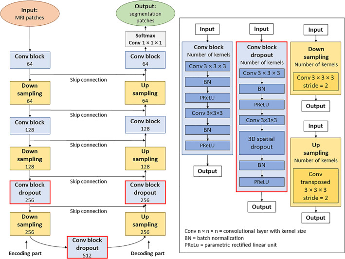
Architecture of the Bayesian U‐Net method using 3D spatial dropout. All investigated Bayesian deep learning methods used a 3D U‐Net as backnone. This 3D U‐Net was considered as a reference method. The architecture of the 3D U‐Net differs from those of the Bayesian methods by not using dropout techniques in its convolutional blocks

2.3.4. Ensemble learning using several 3D DenseNets and 3D U‐Nets

Ensemble learning methods aim to independently train several machine learning models and to combine the models' predictions to obtain accurate and robust results. The machine learning model used to build our ensemble learning method were two 3D DenseNets and two 3D U‐Nets. The architectures of these deep learning networks were identical to those of the previously described 3D DenseNet and 3D U‐Net. To combine the predictions of the 3D DenseNets and 3D U‐Nets, their probability segmentation maps were averaged per voxel.

2.3.5. 3D Bayesian U‐Net

Bayesian neural networks (BNNs) are stochastic artificial neural networks trained using Bayesian inference (Hoffman, Blei, Wang, & Paisley, 2013; MacKay, 1992; Paisley, Blei, & Jordan, 2012). BNNs integrate prior beliefs about the network weights and assess neural network uncertainty. For this purpose, prior distributions are placed over the network weights and stochastic predictions are performed using posterior inference. Unfortunately, Bayesian inference with neural networks is intractable and ipso facto highly challenging to apply in several scientific fields (e.g., medical image processing, autonomous driving, reinforcement learning). To address this issue without reducing network complexity and performance, Gal et al. approximated BNNs using a Monte Carlo Dropout algorithm (Gal & Ghahramani, 2016). In this method, dropout (Srivastava, Hinton, Krizhevsky, Sutskever, & Salakhutdinov, 2014) was placed over each weighted layer (therefore simulating a Bernoulli prior distribution) and enabled at testing time to allow generation of $T$ stochastic predictions per testing data. Then, the mean and the variance of the stochastic predictions were considered as the model expectation (the final prediction) and the model uncertainty.

3D Bayesian U‐Net using 3D spatial dropout

In our study, Monte Carlo dropout was used to automatically segment the lateral ventricles and surrounding brain tissues of our subjects and to assess model uncertainty (i.e., uncertainty map). For this purpose, 3D spatial dropout was placed over the last convolutional layer of the third, fourth, and fifth convolutional blocks of the previously described 3D U‐Net. Then, the modified neural network (Figure 1) was trained. Further, the 3D spatial dropouts were enabled at testing time and $T$ stochastic forward passes were performed through the trained network to obtain the model expectation (final segmentation) and the uncertainty map of each subject.

The model expectation was defined as:

$${\rm E}=\frac{1}{T}\sum _{t=1}^T{P}_t$$

where $P_t$ represents the probability segmentation map obtained at the t ^th forward pass through the network, and $T$ represents the total number of stochastic forward passes.

The uncertainty map was defined as the entropy of the probability segmentation maps:

$$U=-\sum _i\left(\frac{1}{T}\sum _{t=1}^T{P}_{t,i}\right)\log \left(\frac{1}{T}\sum _{t=1}^T{P}_{t,i}\right)$$

where $P_{t,i}$ represents the probability segmentation map for the volume‐of‐interest i at the t ^th forward pass through the network, and $T$ represents the total number of stochastic forward passes.

A manual grid search was conducted to find the 3D spatial dropout parameter p value producing the most accurate segmentations and uncertainty maps. For this purpose, the 3D Bayesian U‐Net was trained several times with distinct p values: 0.1, 0.2, 0.3, 0.4 and 0.5. Then, the obtained segmentations and uncertainty maps were compared. During the training of the network, p was fixed to the same value in all convolutional blocks.

3D Bayesian U‐Net using 3D spatial concrete dropout

The manual grid search described previously was computationally expensive and did not consider all possible p values. Thus, alternatively, we implemented a 3D Bayesian U‐Net method using 3D spatial concrete dropout that directly optimized p during training of the neural network. This Bayesian method is an extension for 3D convolutional layers of the Monte Carlo concrete dropout method proposed by Gal et al. (2017). The architecture of this method used as backbone the previously described U‐Net. In this architecture, 3D spatial concrete dropout was placed over the last convolutional layer of all convolutional blocks.

Let $\omega ={\left\{W_l\right\}}_{l=1}^L$ a set of weight matrices of a Bayesian neural network, $L$ the number of layers, $P\left(\omega \right)$ the prior of the neural network, and $\theta ={\left\{p_l\right\}}_{l=1}^L$ a set of dropout parameters, Gal et al. interpreted dropout as an approximate distribution $q_{\theta }\left(\omega \right)$ of $P\left(\omega \right)$. Then, they used the Kullback–Leibler divergence between $q_{\theta }\left(\omega \right)$ and $P\left(\omega \right)$ as a penalization term in the loss function of the neural network to ensure that $q_{\theta }\left(\omega \right)$ does not deviate too far from $P\left(\omega \right)$. This penalized loss function was defined as follows:

$${\widehat{\mathcal{L}}}_{\mathrm{MC}}\left(\theta \right)=-\frac{1}{M}\sum _{i\in S}\log p\left(y_i|f^{\omega }\left(x_i\right)\right)+\frac{1}{M}\mathrm{KL}\left(q_{\theta }\left(\omega \right)‖P\left(\omega \right)\right)$$

where $\theta$ is the parameter to optimize, $M$ is the number of data points, $S$ is a random set of data point indexes, $x_i$ and $f^{\omega }\left(x_i\right)$ are the input and output of the neural network, $y_i$ is the true prediction of $x_i$, and $\mathrm{KL}$ is the Kullback–Leibler divergence.

To allow optimization of $\theta$ through gradient descent, Gal et al. proposed to compute the derivative of the penalized loss function using a stochastic backpropagation (Kingma, Salimans, & Welling, 2015; Rezende, Mohamed, & Wierstra, 2014; Titsias & Lázaro‐Gredilla, 2014). This backpropagation method required that the distribution at hand can be reparametrized in the form of $g\left(\theta ,\epsilon \right)$ where $\theta$ is the distribution's parameter and $\epsilon$ is a random variable not depending on $\theta .$ Unfortunatly, the dropout's discrete Bernoulli distribution could not be expressed in this form. To address this issue, Gal et al. replaced the dropout's discrete Bernoulli distribution by its continuous relaxation called concrete distribution (Jang, Gu, & Poole, 2017; Maddison, Mnih, & Teh, 2017). In our Bayesian method, the concrete distribution was used to entirely mask some 3D feature maps of the network (3D spatial concrete dropout) instead of sparsely masking their voxels as it was originally done by Gal et al.

2.4. Network training and parameters

The DLMs were trained using 3D patches (size = 64 × 64 × 64, stride of sliding window = 14) extracted from the MRIs and the manual segmentations. The Adam algorithm (Kingma & Ba, 2014) was used to optimize the DLM parameters. The parameters of the Adam algorithm were: learning rate $=1\times {10}^{-3}$, ${\beta }_1=0.9$, and ${\beta }_2=0.9.$ The binary cross‐entropy was used as loss function. The DLM batch sizes were equal to 6, and the number of epochs of the DLMs was equal to 100 (with 400 gradient descent steps per epoch). For all Bayesian U‐Net methods, the total number of stochastic forward passes was set to 6 to obtain a computational time suitable for clinical practice. For the Bayesian U‐Net using 3D spatial concrete dropout, the weight and spatial dropout regularizers were set to $1e^{-6}$ and $1e^{-5}$. During the training of the DLMs, on‐the‐fly data augmentation (translation by −5 to +5 mm per axis, rotation by −5° to +5° per axis, vertical flip, and generation of synthetic MRI motion artifacts (Pérez‐García, Sparks, & Ourselin, 2021)) was conducted to make them more robust to overfitting. During testing of the DLMs, the probability segmentation maps obtained from neighbor patches were averaged. Then, majority votes were applied on the average patches to get the segmented patches. All DLMs were implemented on an Nvidia A100 PCIE 40 GB GPU card using Python 3.6.0 and Keras (Chollet, 2015). The training computational times (per fold) of the DenseNet, U‐Net, ensemble learning using several DenseNets and U‐Nets, Bayesian U‐Net using 3D spatial dropout (p = 0.1), and Bayesian U‐Net using 3D spatial concrete dropout were 2.46, 2.73, 10.38, 2.77, and 3.06 hr, respectively. Table 2 summarized the total number of parameters used by each DLM.

2.5. Evaluation of the DLMs

2.5.1. Segmentation endpoints

To evaluate the performance of the proposed DLMs, the manual and DLM segmentations of each volumes‐of‐interest were compared. For this comparison, endpoints such as Dice score, 95^th percentile of the Hausdorff distance (95^th HD), average symmetric surface distance (ASSD), absolute and relative volume differences were considered.

Dice score was defined as:

$$\text{Dice score}\left({\mathrm{Seg}}_{\mathrm{m}},{\mathrm{Seg}}_{\mathrm{d}}\right)=\frac{2\times \left({\mathrm{Seg}}_{\mathrm{m}}\cap {\mathrm{Seg}}_{\mathrm{d}}\right)}{\left|{\mathrm{Seg}}_{\mathrm{m}}\right|+\left|{\mathrm{Seg}}_{\mathrm{d}}\right|}$$

95^th percentile of the Hausdorff distance was defined as:

$${95}^{th}HD\left({\mathrm{Seg}}_{\mathrm{m}},{\mathrm{Seg}}_{\mathrm{d}}\right)={95}^{\mathit{th}}\text{percentile}(\forall {\text{voxel}}_{\mathrm{m}}\in {\mathrm{Seg}}_{\mathrm{m}}\underset{{\text{voxel}}_{\mathrm{d}}\in {\mathrm{Seg}}_{\mathrm{d}}}{\inf }\text{dist}\left({\text{voxel}}_{\mathrm{m}},{\text{voxel}}_{\mathrm{d}}\right),\forall {\text{voxel}}_{\mathrm{d}}\in {\mathrm{Seg}}_{\mathrm{d}}\underset{{\text{voxel}}_{\mathrm{m}}\in {\mathrm{Seg}}_{\mathrm{m}}}{\inf }\text{dist}\left({\text{voxel}}_{\mathrm{d}},{\text{voxel}}_{\mathrm{m}}\right))$$

Average symmetric surface distance was defined as:

$$\text{ASSD}\left({\mathrm{Seg}}_{\mathrm{m}},{\mathrm{Seg}}_{\mathrm{d}}\right)=\frac{1}{\left|{\text{Surf}}_{\mathrm{m}}\right|+\left|{\text{Surf}}_{\mathrm{m}}\right|}\times (\sum _{{\text{vertex}}_{\mathrm{m}}\in {\text{Surf}}_{\mathrm{m}}}\underset{{\text{vertex}}_{\mathrm{d}}\in {\text{Surf}}_{\mathrm{d}}}{\inf }\text{dist}\left({\text{vertex}}_{\mathrm{m}},{\text{vertex}}_{\mathrm{d}}\right)+\sum _{{\text{vertex}}_{\mathrm{d}}\in {\text{Surf}}_{\mathrm{d}}}\underset{{\text{vertex}}_{\mathrm{m}}\in {\text{Surf}}_{\mathrm{m}}}{\inf }\text{dist}\left({\text{vertex}}_{\mathrm{d}},{\text{vertex}}_{\mathrm{m}}\right))$$

Absolute volume difference was defined as:

$$\text{Absolute volume difference}\left({\mathrm{Vol}}_{\mathrm{m}},{\mathrm{Vol}}_{\mathrm{d}}\right)=\left|{\mathrm{Vol}}_{\mathrm{m}}-{\mathrm{Vol}}_{\mathrm{d}}\right|$$

Relative volume difference was defined as:

$$\text{Relative volume difference}\left({\mathrm{Vol}}_{\mathrm{m}},{\mathrm{Vol}}_{\mathrm{d}}\right)=\frac{\left|{\mathrm{Vol}}_{\mathrm{m}}-{\mathrm{Vol}}_{\mathrm{d}}\right|}{\left|{\mathrm{Vol}}_{\mathrm{m}}\right|}$$

where ${\mathrm{Seg}}_{\mathrm{m}}$ and ${\mathrm{Seg}}_{\mathrm{d}}$ are the manual and DLM segmentations, ${\text{Surf}}_{\mathrm{m}}$ and ${\text{Surf}}_{\mathrm{d}}$ are the surfaces of the manual and DLM segmentations, $\text{dist}$ is the Euclidian distance, and ${\mathrm{Vol}}_{\mathrm{m}},{\mathrm{Vol}}_{\mathrm{d}}$ are the volume of the manual and DLM segmentations.

2.5.2. Uncertainty endpoints

To evaluate and compare the uncertainty maps provided by the Bayesian U‐Net methods:

1. Binary error maps between the manual and Bayesian U‐Net segmentations were computed and used as ground truth. Error map value = 1 represents voxels where the manual and Bayesian U‐Net segmentations were distinct, and error map value = 0 represents voxels where the manual and Bayesian U‐Net segmentations were in agreement.

2. Uncertainty maps were normalized between 0 and 1 (per segmentation method).

3. Normalized uncertainty maps were binarized by thresholding, and they were compared to their corresponding error maps using endpoints such as recall, negative predictive value (NPV), accuracy, and area under the receiving operating characteristic curve (AUC) (Mobiny et al., 2021).

Normalization of the uncertainty maps was performed using the following formula:

$$\text{Normalized}\left(U_{\mathrm{k}}\right)=\frac{\left(U_{\mathrm{k}}-U_{\min }\right)}{\left(U_{\max }-U_{\min }\right)}$$

where $U_{\mathrm{k}}$ is the uncertainty map of a given subject for method $k$, and $U_{\max }$ and $U_{\min }$ are the maximum and minimum values of the uncertainty maps across the entire cohort for method $k$. In our experiments, $U_{\min }$ was set to 0 as the uncertain map values (corresponding to entropy values) cannot be lower than 0.

The threshold values used to binarize the uncertainty maps were determined using the geometric mean metric. This metric was defined as:

$$\text{gmean}\left(U_{\mathrm{k},\mathrm{i}}\right)=\sqrt{\text{recall}\left(U_{\mathrm{k},\mathrm{i}},E_{\mathrm{k}}\right)\times \left(1-\mathrm{FPR}\left(U_{k,i},E_k\right)\right)}$$

where $U_{\mathrm{k},i}$ and $E_{\mathrm{k}}$ are the binarized uncertainty and error maps of a given subject for method $k$, $i\in ⟦0;1⟧$ is the threshold value used to binarize $U_{k,i}$, and $\mathit{FPR}$ is the false positive rate.

The $\underset{i}{\text{argmax}}\text{gmean}\left(U_{k,i}\right)$ allows finding of an optimal threshold $i_{\mathrm{opt}}$ that balance $\text{recall}\left(U_{\mathrm{k}},E_{\mathrm{k}}\right)$ and $\mathit{FPR}\left(U_{\mathrm{k}},E_{\mathrm{k}}\right)$ of a given subject. The optimal thresholds of all subjects were calculated using $\underset{i}{\text{argmax}}\text{gmean}$ and average over the entire cohort per method (values of $i$ tested to estimate $i_{\mathrm{opt}}$ ranged between 0 and 1 with a step = 0.01). Then, the obtained average thresholds were used to binarize the uncertainty maps of all subjects (per method) and to compute the uncertainty endpoint values.

Recall represents the probability that the model is uncertain about its prediction given its prediction is incorrect. It was defined as:

$$\text{recall}=P\left(\text{uncetain}|\text{incorrect}\right)=\frac{P\left(\text{uncertain},\text{incorrect}\right)}{P\left(\text{incorrect}\right)}=\frac{\mathrm{tp}}{\left(\mathrm{tp}+\mathrm{fn}\right)}$$

FPR was defined as:

$$\mathrm{FPR}=\frac{\mathit{fp}}{\left(\mathit{fp}+\mathit{tn}\right)}$$

NPV represents the probability that the model prediction is correct given the model is certain about its prediction. It was defined as:

$$\mathrm{NPV}=P\left(\text{correct}|\text{certain}\right)=\frac{P\left(\text{correct},\text{certain}\right)}{P\left(\text{certain}\right)}=\frac{\mathit{tn}}{\left(\mathit{tn}+\mathit{fn}\right)}$$

Accuracy is the ratio of the number of voxels where the uncertainty and error maps were in agreement over the total number of voxels. It was defined as:

$$\text{Accuracy}=\frac{\mathit{tp}+\mathit{tn}}{\mathit{tp}+\mathit{fp}+\mathit{tn}+\mathit{fn}}$$

where $\mathit{tp}$ is the number of true positives, $\mathit{fp}$ is the number of false positives, $\mathit{fn}$ is the number of false negatives, and $\mathit{tn}$ is the number of true negatives.

AUC is the area under the receiving operating characteristic curve computed from recall and FPR.

2.5.3. Stability of the segmentation and uncertainty results of the Bayesian U‐Net using 3D spatial dropout and Bayesian U‐Net using 3D spatial concrete dropout

The 4‐fold cross‐validation performed with the Bayesian U‐Net using 3D spatial dropout (p = 0.1) and Bayesian U‐Net using 3D spatial concrete dropout was repeated three times to quantify the stability of the results and stochastic biases of these methods. The means and SDs of the segmentation and uncertainty endpoint values across the repeated cross‐validations were compared (per method and volume‐of‐interest).

2.5.4. Robustness to challenging subjects

Cumulative histograms of the Dice scores of the external CSF and lateral ventricles were computed to identify subjects with failed segmentations (Dice scores values < 0.75). The number of subjects with failed segmentations for the DenseNet, U‐Net, ensemble learning using several DenseNets and U‐Nets, Bayesian U‐Net using 3D spatial dropout (p = 0.1), and Bayesian U‐Net using 3D spatial concrete dropout were compared to determine the most robust method.

2.6. Statistical analysis

Paired Wilcoxon tests were used to (a) compare the segmentation endpoint values of the Bayesian U‐Net using 3D spatial dropout (p = 0.1) and Bayesian U‐Net using 3D spatial concrete dropout to those of the other Bayesian U‐Net methods; (b) compare the uncertainty endpoint values of the Bayesian U‐Net using 3D spatial dropout (p = 0.1) and Bayesian U‐Net using 3D spatial concrete dropout to those of the other Bayesian U‐Net methods; (3) compare the segmentation endpoint values of the Bayesian U‐Net using 3D spatial dropout (p = 0.1) and Bayesian U‐Net using 3D spatial concrete dropout to those of the DenseNet, U‐Net, and ensemble learning using several DenseNets and U‐Nets. The endpoint values were considered significantly different when the p‐values of the Wilcoxon tests were less than 0.05.

Friedman tests were used to compare the segmentation and uncertainty endpoint value distributions across the three repeated cross‐validations of the Bayesian U‐Net using 3D spatial dropout (p = 0.1) and Bayesian U‐Net using 3D spatial concrete dropout. The distributions were considered significantly different when the p‐values of the Friedman tests were less than 0.05.

3. RESULTS

3.1. Optimization of the Bayesian U‐Net using 3D spatial dropout through manual grid search

Table 3. shows the mean segmentation endpoint values of all Bayesian U‐Net methods and volumes‐of‐interest. Overall, the Bayesian U‐Net using 3D spatial dropout with p = 0.1 provided significantly higher Dice score values and lowest 95^th HD, ASSD, absolute and relative volume difference values than other Bayesian U‐Net methods using 3D spatial dropout. The Bayesian U‐Net using 3D spatial dropout with p = 0.5 provided the lowest Dice score values and the highest 95^th HD, and ASSD values. Table 4 shows the mean uncertainty endpoint values of the Bayesian U‐Net methods. All methods provided high uncertainty endpoint values (which demonstrates good concordance between the uncertainty maps and their corresponding error maps). Overall, the accuracy and AUC values of the Bayesian U‐Net using 3D spatial dropout with p = 0.1 were significantly higher than those of the other Bayesian U‐Net methods using 3D spatial dropout. Figure 2 shows the segmentations and uncertainty maps of one subject for all Bayesian U‐Nets using 3D spatial dropout. Visual inspection of these images showed qualitative differences across the Bayesian U‐Net segmentations. The Bayesian U‐Net using 3D spatial dropout with p = 0.1 produced the segmentation closest to the manual segmentation. All the Bayesian U‐Net uncertainty maps accurately highlighted areas where the segmentation failed. The hotspots (i.e., highly mislabeled areas) on these uncertainty maps were mainly localized in the inferior medial temporal regions, the inferior part of the brainstem, the cerebellum, and the hippocampal areas. The uncertainty map of the Bayesian U‐Net using 3D spatial dropout with p = 0.1 showed fewer hotspots than those of the other Bayesian methods using 3D spatial dropout.

TABLE 3.

Segmentation endpoint values for all Bayesian U‐Net methods and volumes‐of‐interest

	Lateral ventricles	External CSF	White matter	Cortical gray matter	Cerebellum	Brainstem
Dice score (ratio)
Bayesian U‐Net using 3D spatial concrete dropout	0.948 (± 0.034)	0.823 (± 0.114)	0.900* (± 0.054)	0.840* (± 0.085)	0.907 (± 0.061)	0.900* (± 0.033)
Bayesian U‐Net using 3D spatial dropout (p = 0.1)	0.942 (± 0.052)	0.820 (± 0.112)	0.901 (± 0.053)	0.846 (± 0.080)	0.904 (± 0.061)	0.906 (± 0.033)
Bayesian U‐Net using 3D spatial dropout (p = 0.2)	0.946 (± 0.411)	0.818 (± 0.115)	0.896* (± 0.058)	0.839* (± 0.087)	0.910 (± 0.057)	0.902* (± 0.037)
Bayesian U‐Net using 3D spatial dropout (p = 0.3)	0.911+ (± 0.132)	0.819+ (± 0.112)	0.893*+ (± 0.057)	0.835* (± 0.085)	0.897+ (± 0.074)	0.898 (± 0.042)
Bayesian U‐Net using 3D spatial dropout (p = 0.4)	0.935*+ (± 0.061)	0.821 (± 0.113)	0.893*+ (± 0.058)	0.831* (± 0.097)	0.900 (± 0.075)	0.901* (± 0.036)
Bayesian U‐Net using 3D spatial dropout (p = 0.5)	0.922*+ (± 0.105)	0.814+ (± 0.119)	0.892*+ (± 0.057)	0.832* (± 0.090)	0.892* (± 0.091)	0.899* (± 0.037)
95th Hausdorff distance (mm)
Bayesian U‐Net using 3D spatial concrete dropout	1.357 (± 2.131)	1.973 (± 1.849)	1.226 (± 0.849)	1.130* (± 0.841)	2.365 (± 5.064)	2.087 (± 3.868)
Bayesian U‐Net using 3D spatial dropout (p = 0.1)	3.108 (± 8.631)	2.837 (± 4.839)	1.193 (± 0.769)	1.076 (± 0.768)	1.658 (± 0.836)	2.001 (± 3.904)
Bayesian U‐Net using 3D spatial dropout (p = 0.2)	2.961 (± 8.540)	2.964 (± 5.118)	1.240* (± 0.748)	1.147* (± 0.878)	2.598 (± 5.489)	2.565* (± 4.975)
Bayesian U‐Net using 3D spatial dropout (p = 0.3)	4.835*+ (± 10.280)	2.053 (± 1.935)	1.278*+ (± 0.774)	1.133* (± 0.827)	1.759 (± 1.047)	2.133* (± 3.963)
Bayesian U‐Net using 3D spatial dropout (p = 0.4)	3.120+ (± 8.187)	3.097 (± 6.048)	1.261*+ (± 0.761)	1.161* (± 0.848)	1.762 (± 1.359)	2.058 (± 3.955)
Bayesian U‐Net using 3D spatial dropout (p = 0.5)	4.694*+ (± 11.853)	3.361 (± 6.162)	1.315*+ (± 0.747)	1.223* (± 0.906)	1.886*+ (± 1.142)	2.150* (± 3.965)
Average symmetric surface distance (mm)
Bayesian U‐Net using 3D spatial concrete dropout	0.371 (± 0.302)	0.458 (± 0.390)	0.346 (± 0.194)	0.293* (± 0.162)	0.651 (± 0.613)	0.507* (± 0.395)
Bayesian U‐Net using 3D spatial dropout (p = 0.1)	0.336 + (± 1.372)	0.194 (± 0.502)	0.249 (± 0.201)	0.203 (± 0.225)	0.394 (± 0.270)	0.442 (± 0.334)
Bayesian U‐Net using 3D spatial dropout (p = 0.2)	0.482 (± 0.882)	0.526 (± 0.557)	0.373* (± 0.215)	0.327* (± 0.201)	0.676 (± 0.742)	0.487* (± 0.400)
Bayesian U‐Net using 3D spatial dropout (p = 0.3)	0.790 (± 1.271)	0.461 (± 0.377)	0.369*+ (± 0.201)	0.318*+ (± 0.175)	0.574 (± 0.332)	0.460 (± 0.344)
Bayesian U‐Net using 3D spatial dropout (p = 0.4)	0.537+ (± 0.827)	0.554 (± 0.674)	0.378*+ (± 0.207)	0.322*+ (± 0.184)	0.594 (± 0.437)	0.500* (± 0.385)
Bayesian U‐Net using 3D spatial dropout (p = 0.5)	1.04*+ (± 2.615)	0.594 (± 0.770)	0.395*+ (± 0.221)	0.368*+ (± 0.287)	0.631* (± 0.457)	0.530* (± 0.480)
Absolute volume difference (cm3)
Bayesian U‐Net using 3D spatial concrete dropout	1.594 (± 1.893)	6.562 (± 6.473)	7.917 (± 7.955)	6.785 (± 6.389)	0.894 (± 1.158)	0.410* (± 0.353)
Bayesian U‐Net using 3D spatial dropout (p = 0.1)	1.691 (± 2.001)	8.507+ (± 7.952)	7.211 (± 8.616)	5.907 (± 6.714)	1.088+ (± 1.191)	0.262 (± 0.268)
Bayesian U‐Net using 3D spatial dropout (p = 0.2)	1.503 (± 1.839)	8.858+ (± 8.916)	9.280* (± 11.135)	7.893* (± 9.265)	0.930 (± 1.084)	0.317* (± 0.269)
Bayesian U‐Net using 3D spatial dropout (p = 0.3)	3.179 (± 6.103)	8.131+ (± 8.429)	8.946* (± 9.209)	7.204 (± 6.858)	1.313*+ (± 1.488)	0.402* (± 0.441)
Bayesian U‐Net using 3D spatial dropout (p = 0.4)	2.382*+ (± 2.430)	8.118+ (± 7.560)	9.857*+ (± 11.123)	7.858* (± 9.294)	1.057 (± 1.456)	0.342 (± 0.331)
Bayesian U‐Net using 3D spatial dropout (p = 0.5)	2.490*+ (± 2.927)	8.826+ (± 8.002)	9.425* (± 11.384)	7.748* (± 9.213)	1.291*+ (± 1.516)	0.328 (± 0.333)
Relative volume difference (ratio)
Bayesian U‐Net using 3D spatial concrete dropout	0.038 (± 0.047)	0.106 (± 0.115)	0.068 (± 0.062)	0.071* (± 0.057)	0.077 (± 0.090)	0.090* (± 0.077)
Bayesian U‐Net using 3D spatial dropout (p = 0.1)	0.046 (± 0.065)	0.130 (± 0.121)	0.062+ (± 0.070)	0.061 (± 0.059)	0.098+ (± 0.105)	0.056 (± 0.060)
Bayesian U‐Net using 3D spatial dropout (p = 0.2)	0.035 (± 0.036)	0.135 (± 0.137)	0.080*+ (± 0.087)	0.081* (± 0.085)	0.078 (± 0.083)	0.070* (± 0.060)
Bayesian U‐Net using 3D spatial dropout (p = 0.3)	0.176 (± 0.496)	0.121 (± 0.131)	0.077* (± 0.073)	0.074* (± 0.059)	0.114+ (± 0.123)	0.082* (± 0.080)
Bayesian U‐Net using 3D spatial dropout (p = 0.4)	0.066*+ (± 0.091)	0.128+ (± 0.135)	0.086*+ (± 0.091)	0.083* (± 0.089)	0.089 (± 0.112)	0.070 (± 0.058)
Bayesian U‐Net using 3D spatial dropout (p = 0.5)	0.157* (± 0.313)	0.147+ (± 0.163)	0.083* (± 0.098)	0.080* (± 0.085)	0.115+ (± 0.140)	0.068 (± 0.064)

Note: Values of the segmentation endpoints are presented as mean ± standard deviation (over the entire cohort). Highest Dice score values and lowest 95^th Hausdorff distance, average symmetric surface distance, absolute and relative volume difference values are shown in bold. p represents the value of the dropout parameter used in the Bayesian U‐Net methods. Wilcoxon tests were used to compare the segmentation endpoint values of the Bayesian U‐Net using 3D spatial dropout with p = 0.1 to those of the other Bayesian U‐Net methods (alternative hypothesis was set to “greater” for the Dice score and “smaller” for the other endpoints). Significant differences (p‐values < 0.05) are displayed with (*). Wilcoxon tests were also used to compare the segmentation endpoint values of the Bayesian U‐Net using 3D spatial concrete dropout to those of the other Bayesian U‐Net methods (alternative hypothesis was set to “greater” for the Dice score and “smaller” for the other endpoints). Significant differences (p‐values < 0.05) are displayed with (+).

TABLE 4.

Uncertainty endpoint values for all Bayesian U‐Net methods

	Recall	NPV	Accuracy	AUC
Bayesian U‐Net using 3D spatial concrete dropout	0.953 (± 0.037)	0.998 (± 0.005)	0.906* (± 0.032)	0.949 (± 0.031)
Bayesian U‐Net using 3D spatial dropout (p = 0.1)	0.953 (± 0.032)	0.998 (± 0.004)	0.908 (± 0.030)	0.941+ (± 0.026)
Bayesian U‐Net using 3D spatial dropout (p = 0.2)	0.951 (± 0.038)	0.998 (± 0.005)	0.906* (± 0.029)	0.900*+ (± 0.048)
Bayesian U‐Net using 3D spatial dropout (p = 0.3)	0.955 (± 0.034)	0.999 (± 0.005)	0.903* (± 0.029)	0.914*+ (± 0.056)
Bayesian U‐Net using 3D spatial dropout (p = 0.4)	0.956 (± 0.033)	0.998 (± 0.004)	0.905* (± 0.025)	0.956 (± 0.020)
Bayesian U‐Net using 3D spatial dropout (p = 0.5)	0.955 (± 0.031)	0.998 (± 0.004)	0.903* (± 0.029)	0.917*+ (± 0.049)

Note: Values of the uncertainty endpoints are presented as mean ± SD (over the entire cohort). Highest values are shown in bold. p represents the value of the dropout parameter used in the Bayesian U‐Net methods. Wilcoxon tests were used to compare the uncertainty endpoint values of the Bayesian U‐Net using 3D spatial dropout with p = 0.1 to those of the other Bayesian U‐Net methods (alternative hypothesis was set to “greater” for all endpoints). Significant differences (p‐values < 0.05) are displayed with (*). Wilcoxon tests were also used to compare the uncertainty endpoint values of the Bayesian U‐Net using 3D spatial concrete dropout to those of the other Bayesian U‐Net methods (alternative hypothesis was set to “greater” for all endpoints). Significant differences (p‐values < 0.05) are displayed with (+).

FIGURE 2.

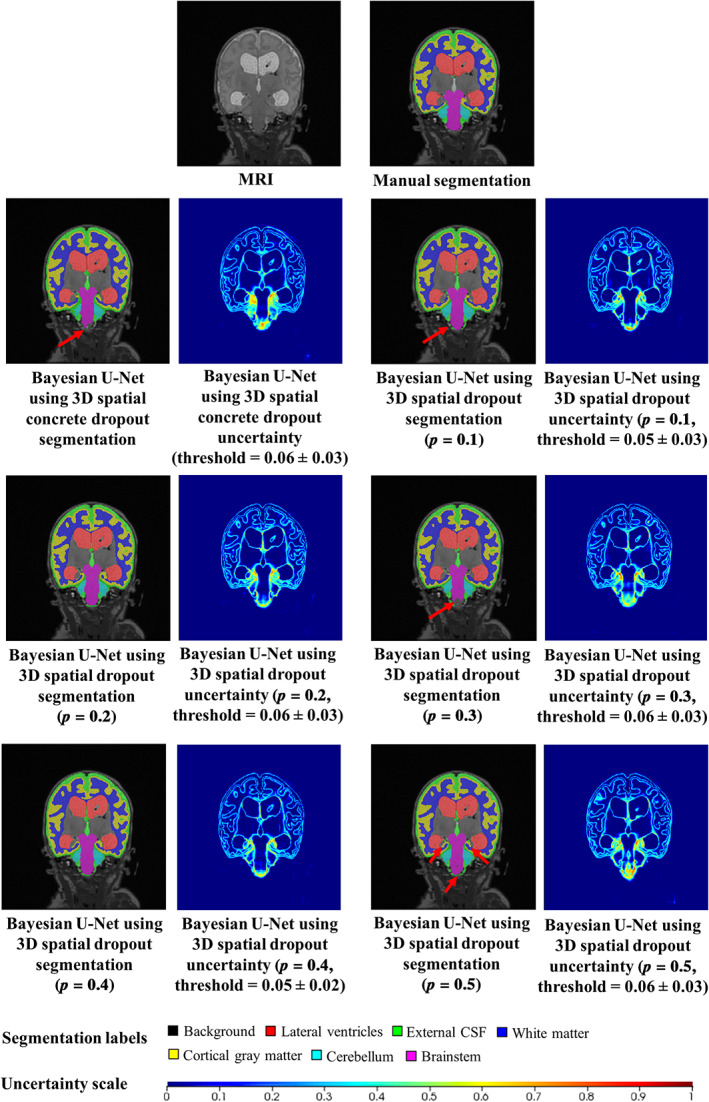
Example of the segmentations and uncertainty maps of one subject for all Bayesian U‐Net methods. The selected subject was the one with the highest AUC values (uncertainty endpoint) for the Bayesian U‐Net using 3D spatial dropout (p = 0.1) and the Bayesian U‐Net using 3D spatial concrete dropout. The AUC values of this subject for the Bayesian U‐Net using 3D spatial concrete dropout and the Bayesian U‐Net using 3D spatial dropout with p = 0.1, 0.2, 0.3, 0.4, and 0.5 were equal to 0.980, 0.975, 0.964, 0.975, 0.977, and 0.965. Uncertainty voxels < threshold indicate where the model is certain about this prediction. Uncertainty voxels > threshold indicate where the model is uncertain about this prediction

3.2. Comparison between the Bayesian U‐Net using 3D spatial dropout (p = 0.1) and the Bayesian U‐Net using 3D spatial concrete dropout

In the lateral ventricles and external CSF, the Bayesian U‐Net using 3D spatial concrete dropout provided higher Dice score values and lower 95^th HD, absolute and relative volume difference values than the Bayesian U‐Net using 3D spatial dropout with p = 0.1 (Table 3). Conversely, the Bayesian U‐Net using 3D spatial dropout with p = 0.1 showed higher Dice score values and lower 95^th HD, ASSD, absolute and relative volume difference values than the Bayesian U‐Net using 3D spatial concrete dropout in the white matter, cortical gray matter, and brainstem. The Bayesian U‐Net using 3D spatial concrete dropout and Bayesian U‐Net using 3D spatial dropout with p = 0.1 presented comparable uncertainty endpoint values (Table 4). For the subject in Figure 2, the uncertainty map of the Bayesian U‐Net using 3D spatial concrete dropout showed hotspots in similar locations to the one of the Bayesian U‐Net using 3D spatial dropout with p = 0.1. Table 5 shows the spatial dropout parameter p values optimized through the Bayesian U‐Net using 3D spatial concrete dropout. These optimized p values were noticeably close to zero in the convolutional blocks 1, 2, 6, and 7 (those extracting low semantic information) and ranged between 0.007 and 0.363 in the convolutional blocks 3, 4, 5 (those extracting high semantic information). Table 6. shows the segmentation endpoint values of the three repeated 4‐fold cross‐validations performed with the Bayesian U‐Net using 3D spatial dropout with p = 0.1 and the Bayesian U‐Net using 3D spatial concrete dropout. For both methods, the standard deviations (stochastic biases) of the segmentation endpoint values across the repeated cross‐validations were low (which indicates overall stable segmentation results). The distributions of the segmentation endpoint values (per method and volume‐of‐interest) were not significantly different (except in the lateral ventricles for the Bayesian U‐Net using 3D spatial concrete dropout). Table 7 shows the uncertainty endpoint values of the three repeated 4‐fold cross‐validations performed with the Bayesian U‐Net using 3D spatial dropout with p = 0.1 and the Bayesian U‐Net using 3D spatial concrete dropout. The standard deviations (stochastic biases) of the uncertainty endpoint values across the repeated cross‐validations were low for both methods. The distributions of the uncertainty endpoint values (per method and volume‐of‐interest) were not significantly different (except for the AUC).

TABLE 5.

Values of the spatial dropout parameter p optimized through the Bayesian U‐Net using 3D spatial concrete dropout for each cross‐validation fold

	Fold 1	Fold 2	Fold 3	Fold 4
Value of p in convolutional block 1	0.000	0.000	0.000	0.000
Value of p in convolutional block 2	0.000	0.000	0.002	0.000
Value of p in convolutional block 3	0.153	0.158	0.158	0.027
Value of p in convolutional block 4	0.304	0.254	0.270	0.363
Value of p in convolutional block 5	0.046	0.047	0.106	0.007
Value of p in convolutional block 6	0.000	0.000	0.000	0.000
Value of p in convolutional block 7	0.000	0.000	0.000	0.000

TABLE 6.

Stability of the segmentation results of the Bayesian U‐Net using 3D spatial dropout (p = 0.1) and Bayesian U‐Net using 3D spatial concrete dropout

	Lateral ventricles	External CSF	White matter	Cortical gray matter	Cerebellum	Brainstem
Dice score (ratio)
Bayesian U‐Net using 3D spatial dropout 1 (p = 0.1)	0.945 (± 0.039)	0.814 (± 0.122)	0.898 (± 0.056)	0.838 (± 0.089)	0.886 (± 0.108)	0.897 (± 0.050)
Bayesian U‐Net using 3D spatial dropout 2 (p = 0.1)	0.942 (± 0.052)	0.820 (± 0.112)	0.901 (± 0.053)	0.846 (± 0.080)	0.904 (± 0.061)	0.906 (± 0.033)
Bayesian U‐Net using 3D spatial dropout 3 (p = 0.1)	0.948 (± 0.034)	0.821 (± 0.112)	0.899 (± 0.058)	0.844 (± 0.087)	0.905 (± 0.061)	0.905 (± 0.032)
Bayesian U‐Net using 3D spatial dropout (p = 0.1) mean	0.945 (± 0.003)	0.818 (± 0.004)	0.899 (± 0.002)	0.843 (± 0.004)	0.898 (± 0.011)	0.902 (± 0.005)
Bayesian U‐Net using 3D spatial concrete dropout 1	0.948 (± 0.034)	0.823 (± 0.114)	0.900 (± 0.054)	0.840 (± 0.085)	0.907 (± 0.061)	0.900 (± 0.033)
Bayesian U‐Net using 3D spatial concrete dropout 2	0.946 (± 0.036)	0.819 (± 0.114)	0.898 (± 0.059)	0.836 (± 0.086)	0.905 (± 0.068)	0.901 (± 0.031)
Bayesian U‐Net using 3D spatial concrete dropout 3	0.942 (± 0.035)	0.819 (± 0.109)	0.895 (± 0.057)	0.838 (± 0.084)	0.908 (± 0.048)	0.900 (± 0.038)
Bayesian U‐Net using 3D spatial concrete dropout mean	0.945* (± 0.003)	0.820 (± 0.002)	0.898 (± 0.003)	0.838 (± 0.002)	0.907 (± 0.002)	0.900 (± 0.001)
95th Hausdorff distance (mm)
Bayesian U‐Net using 3D spatial dropout 1 (p = 0.1)	2.620 (± 6.575)	3.267 (± 6.181)	1.198 (± 0.737)	1.606 (± 3.168)	3.891 (± 8.214)	2.720 (± 5.435)
Bayesian U‐Net using 3D spatial dropout 2 (p = 0.1)	3.108 (± 8.631)	2.837 (± 4.839)	1.193 (± 0.769)	1.076 (± 0.768)	1.658 (± 0.836)	2.001 (± 3.904)
Bayesian U‐Net using 3D spatial dropout 3 (p = 0.1)	1.096 (± 0.808)	2.027 (± 1.859)	1.200 (± 0.796)	1.079 (± 0.778)	1.698 (± 0.971)	2.068 (± 3.949)
Bayesian U‐Net using 3D spatial dropout (p = 0.1) mean	2.275* (± 1.050)	2.710 (± 0.630)	1.197 (± 0.004)	1.254* (± 0.305)	2.416 (± 1.278)	2.263 (± 0.398)
Bayesian U‐Net using 3D spatial concrete dropout 1	1.357 (± 2.131)	1.973 (± 1.849)	1.226 (± 0.849)	1.130 (± 0.841)	2.365 (± 5.064)	2.087 (± 3.868)
Bayesian U‐Net using 3D spatial concrete dropout 2	1.197 (± 1.099)	3.010 (± 5.446)	1.233 (± 0.729)	1.115 (± 0.885)	3.086 (± 7.235)	2.130 (± 3.879)
Bayesian U‐Net using 3D spatial concrete dropout 3	2.575 (± 6.150)	2.927 (± 5.277)	1.238 (± 0.794)	1.123 (± 0.822)	3.183 (± 7.561)	2.084 (± 4.059)
Bayesian U‐Net using 3D spatial concrete dropout mean	1.710* (± 0.754)	2.637* (± 0.576)	1.232 (± 0.006)	1.123 (± 0.008)	2.878 (± 0.447)	2.100 (± 0.026)
Average symmetric surface distance (mm)
Bayesian U‐Net using 3D spatial dropout 1 (p = 0.1)	0.429 (± 0.519)	0.595 (± 0.759)	0.374 (± 0.222)	0.375 (± 0.346)	1.092 (± 1.992)	0.540 (± 0.469)
Bayesian U‐Net using 3D spatial dropout 2 (p = 0.1)	0.336 (± 1.372)	0.194 (± 0.502)	0.249 (± 0.201)	0.203 (± 0.225)	0.394 (± 0.270)	0.442 (± 0.334)
Bayesian U‐Net using 3D spatial dropout 3 (p = 0.1)	0.326 (± 0.198)	0.459 (± 0.365)	0.341 (± 0.206)	0.289 (± 0.158)	0.559 (± 0.304)	0.447 (± 0.317)
Bayesian U‐Net using 3D spatial dropout (p = 0.1) mean	0.363* (± 0.057)	0.416 (± 0.204)	0.321 (± 0.065)	0.289* (± 0.086)	0.682 (± 0.365)	0.476 (± 0.055)
Bayesian U‐Net using 3D spatial concrete dropout 1	0.371 (± 0.302)	0.458 (± 0.390)	0.346 (± 0.194)	0.293 (± 0.162)	0.651 (± 0.613)	0.507 (± 0.395)
Bayesian U‐Net using 3D spatial concrete dropout 2	0.369 (± 0.309)	0.545 (± 0.623)	0.373 (± 0.216)	0.326 (± 0.216)	0.728 (± 1.101)	0.513 (± 0.472)
Bayesian U‐Net using 3D spatial concrete dropout 3	0.476 (± 0.538)	0.502 (± 0.508)	0.354 (± 0.192)	0.322 (± 0.173)	0.686 (± 0.786)	0.486 (± 0.366)
Bayesian U‐Net using 3D spatial concrete dropout mean	0.405* (± 0.061)	0.502 (± 0.044)	0.358 (± 0.014)	0.314 (± 0.018)	0.688 (± 0.039)	0.502 (± 0.014)
Absolute volume difference (cm3)
Bayesian U‐Net using 3D spatial dropout 1 (p = 0.1)	1.594 (± 1.869)	9.604 (± 9.014)	8.258 (± 9.174)	6.559 (± 8.675)	0.937 (± 0.960)	0.338 (± 0.290)
Bayesian U‐Net using 3D spatial dropout 2 (p = 0.1)	1.691 (± 2.001)	8.507 (± 7.952)	7.211 (± 8.616)	5.907 (± 6.714)	1.088 (± 1.191)	0.262 (± 0.268)
Bayesian U‐Net using 3D spatial dropout 3 (p = 0.1)	1.596 (± 1.714)	8.612 (± 8.671)	7.505 (± 10.196)	5.754 (± 7.874)	1.167 (± 1.333)	0.364 (± 0.325)
Bayesian U‐Net using 3D spatial dropout (p = 0.1) mean	1.627 (± 0.055)	8.908 (± 0.605)	7.658 (± 0.540)	6.073 (± 0.428)	1.064 (± 0.117)	0.321* (± 0.053)
Bayesian U‐Net using 3D spatial concrete dropout 1	1.594 (± 1.893)	6.562 (± 6.473)	7.917 (± 7.955)	6.785 (± 6.389)	0.894 (± 1.158)	0.410 (± 0.353)
Bayesian U‐Net using 3D spatial concrete dropout 2	1.592 (± 2.234)	7.697 (± 7.328)	9.639 (± 12.120)	8.399 (± 10.332)	0.915 (± 0.907)	0.372 (± 0.325)
Bayesian U‐Net using 3D spatial concrete dropout 3	2.722 (± 3.390)	8.331 (± 8.189)	7.847 (± 10.029)	6.348 (± 8.180)	0.951 (± 0.964)	0.440 (± 0.442)
Bayesian U‐Net using 3D spatial concrete dropout mean	1.969* (± 0.652)	7.530 (± 0.892)	8.468 (± 1.015)	7.177 (± 1.080)	0.920 (± 0.029)	0.407 (± 0.034)
Relative volume difference (ratio)
Bayesian U‐Net using 3D spatial dropout 1 (p = 0.1)	0.038 (± 0.037)	0.153 (± 0.167)	0.073 (± 0.072)	0.069 (± 0.079)	0.091 (± 0.116)	0.075 (± 0.078)
Bayesian U‐Net using 3D spatial dropout 2 (p = 0.1)	0.046 (± 0.065)	0.130 (± 0.121)	0.062 (± 0.070)	0.061 (± 0.059)	0.098 (± 0.105)	0.056 (± 0.060)
Bayesian U‐Net using 3D spatial dropout 3 (p = 0.1)	0.038 (± 0.035)	0.132 (± 0.132)	0.066 (± 0.082)	0.063 (± 0.074)	0.103 (± 0.112)	0.077 (± 0.067)
Bayesian U‐Net using 3D spatial dropout (p = 0.1) mean	0.041 (± 0.005)	0.138 (± 0.013)	0.067 (± 0.005)	0.063 (± 0.004)	0.097 (± 0.006)	0.069* (± 0.012)
Bayesian U‐Net using 3D spatial concrete dropout 1	0.038 (± 0.047)	0.106 (± 0.115)	0.068 (± 0.062)	0.071 (± 0.057)	0.077 (± 0.090)	0.090 (± 0.077)
Bayesian U‐Net using 3D spatial concrete dropout 2	0.039 (± 0.043)	0.122 (± 0.127)	0.082 (± 0.096)	0.084 (± 0.090)	0.077 (± 0.062)	0.078 (± 0.059)
Bayesian U‐Net using 3D spatial concrete dropout 3	0.046 (± 0.038)	0.134 (± 0.137)	0.068 (± 0.072)	0.064 (± 0.073)	0.077 (± 0.068)	0.092 (± 0.092)
Bayesian U‐Net using 3D spatial concrete dropout mean	0.041* (± 0.004)	0.121 (± 0.014)	0.072 (± 0.008)	0.073 (± 0.010)	0.308 (± 0.400)	0.087 (± 0.008)

Note: Three repeated 4‐fold cross‐validations were conducted on each Bayesian U‐Net method. The obtained segmentation endpoint values are presented as mean ± SD (over the entire cohort) for each cross‐validation. Highest Dice score values and lowest 95th Hausdorff distance, average symmetric surface distance, absolute and relative volume difference values are shown in bold. Friedman tests were used to compare the distributions of the segmentation endpoint values obtained at each cross‐validation (per Bayesian U‐Net method). Significant differences (p‐values < 0.05) are displayed with (*).

TABLE 7.

Stability of the uncertainty results of the Bayesian U‐Net using 3D spatial dropout (p = 0.1) and Bayesian U‐Net using 3D spatial concrete dropout

	Recall	NPV	Accuracy	AUC
Bayesian U‐Net using 3D spatial dropout 1 (p = 0.1)	0.956 (± 0.033)	0.998 (± 0.004)	0.906 (± 0.032)	0.906 (± 0.064)
Bayesian U‐Net using 3D spatial dropout 2 (p = 0.1)	0.953 (± 0.032)	0.998 (± 0.004)	0.908 (± 0.030)	0.941 (± 0.026)
Bayesian U‐Net using 3D spatial dropout 3 (p = 0.1)	0.950 (± 0.034)	0.998 (± 0.004)	0.909 (± 0.032)	0.925 (± 0.033)
Bayesian U‐Net using 3D spatial dropout (p = 0.1) mean	0.953 (± 0.003)	0.998 (± 0.000)	0.908 (± 0.001)	0.924* (± 0.018)
Bayesian U‐Net using 3D spatial concrete dropout 1	0.953 (± 0.037)	0.998 (± 0.005)	0.906 (± 0.032)	0.949 (± 0.031)
Bayesian U‐Net using 3D spatial concrete dropout 2	0.956 (± 0.034)	0.998 (± 0.005)	0.905 (± 0.024)	0.893 (± 0.090)
Bayesian U‐Net using 3D spatial concrete dropout 3	0.950 (± 0.037)	0.998 (± 0.005)	0.902 (± 0.043)	0.912 (± 0.079)
Bayesian U‐Net using 3D spatial concrete dropout mean	0.953 (± 0.003)	0.998* (± 0.000)	0.902 (± 0.002)	0.912* (± 0.028)

Note: Three repeated 4‐fold cross‐validations were conducted on each Bayesian U‐Net method. The obtained uncertainty endpoint values are presented as mean ± SD (over the entire cohort). Highest values are shown in bold. Friedman tests were used to compare the distributions of the uncertainty endpoint values obtained at each cross‐validation (per Bayesian U‐Net method). Significant differences (p‐values <0.05) are displayed with (*).

3.3. Comparison between the DenseNet, U‐Net, ensemble learning using several DenseNets and U‐Nets, Bayesian U‐Net using 3D spatial dropout (p = 0.1), and Bayesian U‐Net using 3D spatial concrete dropout

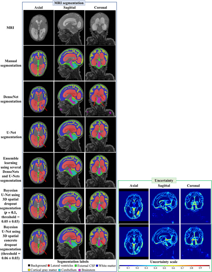
Table 8 shows the segmentation endpoint values of the DenseNet, U‐Net, ensemble learning using several DenseNets and U‐Nets, Bayesian U‐Net using 3D spatial dropout (p = 0.1), and Bayesian U‐Net using 3D spatial concrete dropout for each volume‐of‐interest. Overall, the Bayesian U‐Net methods provided higher Dice score values and lower 95^th HD, ASSD, absolute and relative volume difference values than the DenseNet, U‐Net, and ensemble learning using several DenseNets and U‐Nets. These values were significantly different than those of the DenseNet in each volumes‐of‐interest and those of the ensemble learning using several DenseNets and U‐Nets in the lateral ventricles. The DenseNet provided the lowest Dice score values and highest 95^th HD, ASSD, absolute, and relative volume difference values. Figure 3 shows the DenseNet, U‐Net, Bayesian U‐Net using 3D spatial dropout (p = 0.1), Bayesian U‐Net using 3D spatial concrete dropout segmentations, and the Bayesian U‐Net uncertainty maps of one subject. The Bayesian U‐Net, U‐Net, and ensemble learning using several Dense‐Nets and U‐Nets segmentations were in close agreement with the manual segmentation (except a few discrepancies indicated by the red arrows in Figure 3). Conversely, the DenseNet segmentation presented noticeable mislabeling in the prefrontal white matter, the anterior cingulate, the lateral ventricles, and part of the cerebellum. The Bayesian U‐Net uncertainty maps accurately highlighted the areas where their corresponding segmentations were distinct from the manual segmentation. The hotspots of these uncertainty maps were mostly localized in the inferior medial temporal area, the brainstem, the borders of the lateral ventricles, the periventricular area, and the superior frontal and prefrontal gray matter. The prediction computational times (per subject) of the DenseNet, U‐Net, ensemble learning using several DenseNets and U‐Nets, Bayesian U‐Net using 3D spatial dropout (p = 0.1), and Bayesian U‐Net using 3D spatial concrete dropout were 0.35, 0.38, 1.45, 2.39, and 2.79 min, respectively.

TABLE 8.

Segmentation endpoint values of the DenseNet, U‐Net, ensemble learning using several DenseNets and U‐Nets, and Bayesian U‐Net using 3D spatial dropout (p = 0.1) for each volume‐of‐interest

	Lateral ventricles	External CSF	White matter	Cortical gray matter	Cerebellum	Brainstem
Dice score (ratio)
DenseNet	0.814*+ (± 0.213)	0.732*+ (± 0.136)	0.848*+ (± 0.080)	0.750*+ (± 0.143)	0.527*+ (± 0.233)	0.610*+ (± 0.166)
U‐Net	0.944+ (± 0.041)	0.822 (± 0.110)	0.898* (± 0.057)	0.841* (± 0.084)	0.904 (± 0.062)	0.907 (± 0.033)
Ensemble learning using several DenseNets and U‐Nets	0.942*+ (± 0.042)	0.820 (± 0.111)	0.901 (± 0.054)	0.843 (± 0.086)	0.882* (± 0.095)	0.893 (± 0.060)
Bayesian U‐Net using 3D spatial dropout (p = 0.1)	0.942 (± 0.052)	0.820 (± 0.112)	0.901 (± 0.053)	0.846 (± 0.080)	0.904+ (± 0.061)	0.906 (± 0.033)
Bayesian U‐Net using 3D spatial concrete dropout	0.948 (± 0.034)	0.823 (± 0.114)	0.900* (± 0.054)	0.840* (± 0.085)	0.907 (± 0.061)	0.900* (± 0.033)
95th Hausdorff distance (mm)
DenseNet	11.452*+ (± 10.594)	5.234*+ (± 7.668)	2.264*+ (± 1.555)	2.087*+ (± 1.793)	29.618*+ (± 19.223)	27.258*+ (± 16.143)
U‐Net	2.756 (± 7.703)	2.541 (± 3.877)	1.221 (± 0.766)	1.100 (± 0.838)	1.681 (± 1.054)	2.055 (± 3.967)
Ensemble learning using several DenseNets and U‐Nets	2.341*+ (± 3.860)	3.209+ (± 6.190)	1.193 (± 0.736)	1.102 (± 0.820)	1.928 (± 1.309)	2.128 (± 4.029)
Bayesian U‐Net using 3D spatial dropout (p = 0.1)	3.108 (± 8.631)	2.837 (± 4.839)	1.193 (± 0.769)	1.076 (± 0.768)	1.658 (± 0.836)	2.001 (± 3.904)
Bayesian U‐Net using 3D spatial concrete dropout	1.357 (± 2.131)	1.973 (± 1.849)	1.226 (± 0.849)	1.130* (± 0.841)	2.365 (± 5.064)	2.087 (± 3.868)
Average symmetric surface distance (mm)
DenseNet	2.376*+ (± 2.390)	1.095*+ (± 1.116)	0.676*+ (± 0.413)	0.612*+ (± 0.487)	6.540*+ (± 4.646)	5.456*+ (± 3.784)
U‐Net	0.486 (± 0.818)	0.480 (± 0.445)	0.352 (± 0.204)	0.305* (± 0.174)	0.577 (± 0.425)	0.462 (± 0.352)
Ensemble learning using several DenseNets and U‐Nets	0.449*+ (± 0.396)	0.566 (± 0.691)	0.342 (± 0.188)	0.298* (± 0.165)	0.682* (± 0.561)	0.507* (± 0.393)
Bayesian U‐Net using 3D spatial dropout (p = 0.1)	0.336 + (± 1.372)	0.194 (± 0.502)	0.249 (± 0.201)	0.203 (± 0.225)	0.394 (± 0.270)	0.442(± 0.334)
Bayesian U‐Net using 3D spatial concrete dropout	0.371 (± 0.302)	0.458 (± 0.390)	0.346 (± 0.194)	0.293* (± 0.162)	0.651 (± 0.613)	0.507* (± 0.395)
Absolute volume difference (cm3)
DenseNet	12.671*+ (± 24.936)	15.398*+ (± 17.117)	15.597*+ (± 14.814)	16.439*+ (± 19.628)	4.289*+ (± 3.752)	3.669*+ (± 3.672)
U‐Net	2.051*+ (± 2.666)	7.248+ (± 6.631)	8.465* (± 10.191)	6.977 (± 8.801)	1.147+ (± 1.361)	0.310* (± 0.321)
Ensemble learning using several DenseNets and U‐Nets	2.166*+ (± 2.579)	8.716 (± 8.515)	7.698 (± 8.625)	5.922 (± 7.571)	1.496+ (± 1.865)	0.489* (± 0.631)
Bayesian U‐Net using 3D spatial dropout (p = 0.1)	1.691 (± 2.001)	8.507+ (± 7.952)	7.211 (± 8.616)	5.907 (± 6.714)	1.088+ (± 1.191)	0.262 (± 0.268)
Bayesian U‐Net using 3D spatial concrete dropout	1.594 (± 1.893)	6.562 (± 6.473)	7.917 (± 7.955)	6.785 (± 6.389)	0.894 (± 1.158)	0.410* (± 0.353)
Relative volume difference (ratio)
DenseNet	0.673*+ (± 1.855)	0.235*+ (± 0.306)	0.131*+ (± 0.114)	0.160*+ (± 0.170)	0.368*+ (± 0.302)	0.737*+ (± 0.694)
U‐Net	0.046 (± 0.051)	0.117 (± 0.115)	0.073* (± 0.084)	0.070 (± 0.078)	0.093+ (± 0.099)	0.065 (± 0.073)
Ensemble learning using several DenseNets and U‐Nets	0.054*+ (± 0.068)	0.134+ (± 0.142)	0.068 (± 0.070)	0.064 (± 0.071)	0.128+ (± 0.145)	0.098* (± 0.105)
Bayesian U‐Net using 3D spatial dropout (p = 0.1)	0.046 (± 0.065)	0.130+ (± 0.121)	0.062 (± 0.070)	0.061 (± 0.059)	0.098+ (± 0.105)	0.056 (± 0.060)
Bayesian U‐Net using 3D spatial concrete dropout	0.038 (± 0.047)	0.106 (± 0.115)	0.068 (± 0.062)	0.071* (± 0.057)	0.077 (± 0.090)	0.090* (± 0.077)

Note: Values of the segmentation endpoints are presented as mean ± SD (over the entire cohort). Highest Dice score values and lowest 95th Hausdorff distance, average symmetric surface distance, absolute and relative volume difference values are shown in bold. Wilcoxon tests were used to compare the segmentation endpoint values of the Bayesian U‐Net using 3D spatial dropout (p = 0.1) to those of the other methods (alternative hypothesis is “greater” for the Dice score and “smaller” for the other endpoints). Significant differences (p‐values <0.05) are displayed with (*). Wilcoxon tests were also used to compare the segmentation endpoint values of the Bayesian U‐Net using 3D spatial concrete dropout to those of the other methods (alternative hypothesis was set to “greater” for the Dice score and “smaller” for the other endpoints). Significant differences (p‐values <0.05) are displayed with (+).

FIGURE 3.

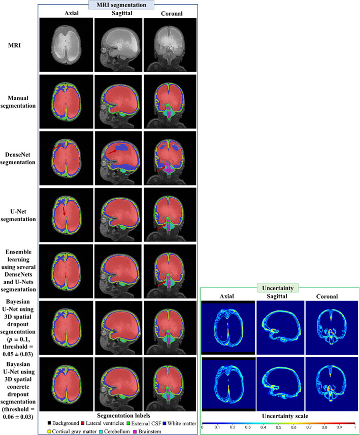
Example of the MRI, the segmentations, and the uncertainty map of one subject for the DenseNet, U‐Net, ensemble learning using several DenseNets and U‐Nets, Bayesian U‐Net using 3D spatial dropout (p = 0.1), and Bayesian U‐Net using 3D spatial concrete dropout. The dice score values of the lateral ventricles of the subject were 0.898, 0.977, 0.980, 0.982, 0.984 for the DenseNet, U‐Net, ensemble learning using several Dense‐Nets and U‐Nets, Bayesian U‐Net using 3D spatial dropout p = 0.1, and Bayesian U‐Net using 3D spatial concrete dropout. Uncertainty voxels < threshold indicate where the model is certain about this prediction. Uncertainty voxels > threshold indicate where the model is uncertain about this prediction

3.4. DenseNet, U‐Net, ensemble learning using several DenseNets and U‐Nets, Bayesian U‐Net using 3D spatial dropout (p = 0.1), and Bayesian U‐Net using 3D spatial concrete dropout robustness to worst cases

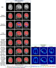
Figures 4 and 5 show the Dice score cumulative histograms computed in the external CSF and lateral ventricles for the DenseNet, U‐Net, ensemble learning using several DenseNets and U‐Nets, Bayesian U‐Net using 3D spatial dropout (p = 0.1), and Bayesian U‐Net using 3D spatial concrete dropout. The numbers of subjects with Dice scores values inferior to 0.75 were lower for the Bayesian U‐Net using 3D spatial concrete dropout compared to the other methods. Visual inspections conducted on these challenging subjects showed that the main differences between their manual and predicted segmentations were mainly localized in the peri/intraventricular area (i.e., areas close to the brain injury and dilated ventricles), the brainstem, and the cerebellum. Figure 6 shows the segmentations provided by the DenseNet, U‐Net, ensemble learning using several DenseNets and U‐Nets, Bayesian U‐Net using 3D spatial dropout (p = 0.1), Bayesian U‐Net using 3D spatial concrete dropout, and the Bayesian U‐Nets’ uncertainty maps of one subject with Dice score values inferior to 0.75 in the external CSF. For this subject, the differences between the manual and deep learning segmentations were localized in the periventricular areas, within the lateral ventricles, the brainstem, and the cerebellum. The uncertainty map of the Bayesian U‐Net using 3D spatial concrete dropout accurately highlighted the areas where its’ corresponding segmentation was distinct from the manual segmentation.

FIGURE 4.

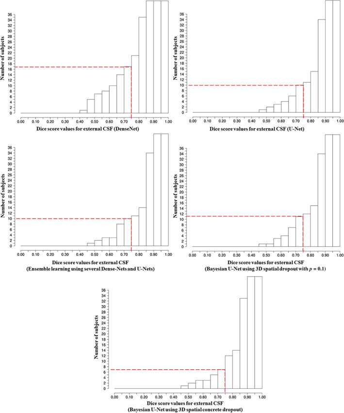
Cumulative histograms of the Dice score of the external CSF for the DenseNet, U‐Net, ensemble learning using several DenseNets and U‐Nets, Bayesian U‐Net using 3D spatial dropout (p = 0.1), and Bayesian U‐Net using 3D spatial concrete dropout. The dashed lines indicate the number of subjects with Dice score of the external CSF and lateral ventricles inferior to 0.75

FIGURE 5.

Cumulative histograms of the Dice score of the lateral ventricles for the DenseNet, U‐Net, ensemble learning using several DenseNets and U‐Nets, Bayesian U‐Net using 3D spatial dropout (p = 0.1), and Bayesian U‐Net using 3D spatial concrete dropout. The dashed lines indicate the number of subjects with Dice score of the external CSF and lateral ventricles inferior to 0.75

FIGURE 6.

Example of a subject with Dice score of the external CSF inferior to 0.75. The dice score values of the external CSF of the subject were 0.572, 0.649, 0.652, 0.642, and 0.665 for the DenseNet, U‐Net, ensemble learning using several DenseNets and U‐Nets, Bayesian U‐Net using 3D spatial dropout with p = 0.1, and Bayesian U‐Net using 3D spatial concrete dropout. Uncertainty voxels < threshold indicate where the model is certain about this prediction. Uncertainty voxels > threshold indicate where the model is uncertain about this prediction

4. DISCUSSION

In this study, we proposed a 3D Bayesian U‐Net using 3D spatial concrete dropout for brain segmentation and uncertainty assessment in preterm infants suffering from post‐hemorrhagic hydrocephalus (PHH). This Bayesian method provided accurate segmentations and uncertainty maps, compared favorably with reference methods such as DenseNet, U‐Net, and ensemble learning using several DenseNets and U‐Nets, and had a computational time suitable for clinical practice.

The manual grid search through the Bayesian U‐Net using 3D spatial dropout showed that the best value for the spatial dropout parameter is p = 0.1, which is consistent with values reported in the adult brain segmentation literature (Jungo, Meier, Ermis, Herrmann, & Reyes, 2018; Roy, Conjeti, Navab, & Wachinger, 2018; Roy, Conjeti, Navab, & Wachinger, 2019). We observed quantitative and qualitative differences across the segmentation results of the Bayesian U‐Nets using 3D spatial dropout. The Bayesian U‐Net using 3D spatial dropout with p = 0.1 provided the outputs closest to the manual segmentation, whereas the results from the Bayesian U‐Net using 3D spatial dropout with p = 0.5 were the furthest from the ground truth. These observations can be explained by the fact that the Bayesian U‐Net using 3D spatial dropout is an efficient ensemble learning method combining results of several U‐Nets where p controls the depth of these networks (and de facto their accuracy and generalization). The uncertainty maps of all Bayesian U‐Nets using spatial dropout accurately highlighted mis‐segmented areas. The uncertainty maps of the Bayesian U‐Net using 3D spatial dropout with p = 0.1 showed fewer hotspots compared to other Bayesian methods using 3D spatial dropout.

The manual grid search through the Bayesian U‐Net using 3D spatial dropout was computationally expensive and did not explore all possible values of p (as p was fixed to the same value in the third, fourth, and fifth convolutional blocks). Due to this fact, we implemented a 3D spatial concrete dropout method that optimizes p directly during training (through gradient descent for all convolutional blocks) and compared results of this method to those of the Bayesian U‐Net using 3D spatial dropout (p = 0.1). We found that the Bayesian U‐Net using 3D spatial concrete dropout provided comparable segmentation and uncertainty results than the Bayesian U‐Net using 3D spatial dropout method (p = 0.1). Both of these Bayesian methods presented stable and consistent segmentation and uncertainty results (i.e., with low stochastic biases across the repeated cross‐validations). The Bayesian U‐Net using 3D spatial concrete dropout appeared nevertheless more robust to challenging subjects than the Bayesian U‐Net using 3D spatial dropout method (p = 0.1). We also found that the dropout parameters of the 3D spatial concrete dropout method were noticeably superior to zero only in the third, fourth, and fifth convolutional blocks. This finding suggests that the uncertainty related to the network weights is mainly localized in the features extracting high semantic information.

We compared the performance of the Bayesian U‐Net using 3D spatial concrete dropout to those of a DenseNet (which showed excellent segmentation results in healthy newborn brains; Bui et al., 2017; Wang et al., 2019), a U‐Net, and an ensemble learning method using several DenseNets and U‐Nets. We found that our Bayesian method provided better segmentation results in the lateral ventricles and external CSF than the DenseNet, U‐Net, and ensemble learning method using several DenseNets and U‐Nets (with competitive segmentation results in other volumes‐of‐interest). Our Bayesian method also showed higher robustness to challenging patients than those methods. This superiority in performance can be explained by the fact that (a) the Bayesian method combines the predictions of several highly accurate U‐Nets as final segmentation result, unlike the DenseNet and U‐Net that outputs only one segmentation prediction; (b) the Bayesian method considered six segmentation predictions to create its final prediction, unlike the ensemble learning method using several DenseNets and U‐Nets which used four segmentation predictions. We also found that our Bayesian method has a higher prediction computational time than the DenseNet, U‐Net, ensemble learning method using several DenseNets and U‐Nets. However, this computational time (2.79 min) was drastically lower than that needed for manual segmentation (which takes at least 1 hr); and adequate since monitoring and making treatment decisions for PHH do not require real‐time segmentation. In clinical applications where real‐time segmentation would have been needed, the Monte Carlo simulation used in the Bayesian method could have been implemented in parallel on the GPU card to decrease its computational time. The Bayesian U‐Net has the advantage over the DenseNet and U‐Net of providing an assessment of its uncertainty. This uncertainty assessment could allow automatic and accurate identification and refinement of errors in the predicted tissue segmentations, and thus increase clinicians' confidence in the segmentation algorithm results (Appendix). The Bayesian method has the advantage over the ensemble learning method using several DenseNets and U‐Nets to provide a considerably lower training computational time and require fewer network parameters. The Bayesian method required the training of one model whereas the ensemble learning method using several DenseNets and U‐Nets required the independent training of four models.

A review of the existing literature on automatic brain segmentation of preterm infants with PHH shows there is a paucity of studies (Gontard et al., 2021; Qiu et al., 2015, 2017; Tabrizi et al., 2018). Tabrizi et al. (2018) reported for the lateral ventricles a mean Dice score equal to 0.800 from 2D ultrasound scans of 60 preterm infants with PHH. Qiu et al. reported for the lateral ventricles a mean Dice score and mean absolute surface distance equal to 0.767 and 1.000 from 3D ultrasound scans of 14 preterm infants with PHH (Qiu et al., 2017), and equal to 0.914 and 2.00 from MRI scans of 7 preterm infants with PHH (Qiu et al., 2015). Gontard et al. (2021) reported for the lateral ventricle a mean Dice score of 0.800 from 3D ultrasound scans of 10 preterm infants with PHH. Our Bayesian U‐Net using 3D spatial concrete dropout showed better performance (with mean Dice score = 0.948 (± 0.034) and mean ASSD = 0.371 (± 0.302), for the lateral ventricles) than methods proposed in previous studies. Our method has the advantage of performing the segmentation of the lateral ventricles and surrounding brain tissues at the same time, unlike previous studies that were focused on segmenting only the ventricles. Our method was trained and evaluated on a larger MRI cohort (including subjects with PHH) compared to Qiu et al. (2015). Additionally, our method provided an assessment of its uncertainty, that has not been previously carried out.

Our study has some limitations. First, our Bayesian U‐Net using 3D spatial concrete dropout was trained on images acquired from two MRI scanners without external validation on images acquired from another MRI scanner, limiting the generalizability of this method across different MRI platforms. Second, we did not evaluate the performance of our Bayesian U‐Net across the two MRI scanners. Third, we did not provide single uncertainty values for each volume‐of‐interest but an uncertainty map. For clinical practice, it may be interesting to provide these single values in addition to the uncertainty map. Finally, we did not demonstrate that the concrete and Bernoulli distributions used for dropout computation are the most suitable for representing the network parameter distributions. Additional investigations are therefore needed and will be part of future work.

5. CONCLUSION

Bayesian U‐Net using 3D spatial concrete dropout provided accurate brain segmentation results and uncertainty assessment in preterm infants diagnosed with PHH. Bayesian U‐Net using 3D spatial concrete dropout compared favorably with reference methods such as DenseNet, U‐Net, and ensemble learning method using several DenseNets and U‐Nets. This method could potentially be incorporated in clinical practice to support more accurate and informed diagnosis, monitoring, and treatment decisions for PHH in preterm infants.

AUTHOR CONTRIBUTIONS

Axel Largent conceived and designed the study, performed the analysis and interpretation of the results, and wrote the article. Josepheen De Asis‐Cruz contributed to the design of the study and analysis and interpretation of the results. Kushal Kapse collected the data. Scott D. Barnett contributed to the statistical analysis. Jonathan Murnick contributed to the interpretation of the results. Sudeepta Basu contributed to the interpretation of the results. Nicole Andersen collected the data. Stephanie Norman collected the data. Nickie Andescavage contributed to the analysis and interpretation of the results and collected the data. Catherine Limperopoulos conceived the study, and contributed to the design of the study, analysis, and interpretation of the results. All authors reviewed the results and approved the final version of the article.

Guideline for localization of mis‐segmented areas with uncertainty maps

The uncertainty maps facilitate the localization of mislabeled brain tissues. Without the uncertainty maps, this localization is time‐consuming, cumbersome, and require very high expertise in anatomy. As currently presented, the uncertainty map is a visualization tool, but nonetheless a tool that could help clinicians focus on problematic regions quickly and provide a quantitative estimate of the segmentation error across the brain.

We propose the operational guidelines below on how to best utilize the uncertainty map to localize mis‐segmented areas:

• Apply the method on given preterm brain MRIs to obtain their segmentations and uncertainty maps.

• Binarize the uncertainty maps using the threshold indicated in the study (0.06). Voxels of the binarized uncertainty maps equal to 1 stand for mis‐segmented areas, and voxels of the binarized uncertainty maps equal to 0 stand for well‐segmented areas.

• Confirm via visual inspections the mis‐segmented areas shown by the binarized uncertainty maps.

• Manually refine the segmentations where mis‐segmented areas were found.

Largent, A. , De Asis‐Cruz, J. , Kapse, K. , Barnett, S. D. , Murnick, J. , Basu, S. , Andersen, N. , Norman, S. , Andescavage, N. , & Limperopoulos, C. (2022). Automatic brain segmentation in preterm infants with post‐hemorrhagic hydrocephalus using 3D Bayesian U‐Net . Human Brain Mapping, 43(6), 1895–1916. 10.1002/hbm.25762

DATA AVAILABILITY STATEMENT

The data used in this study would be made available via request to the corresponding author. This request may be restricted to patient privacy and need of approval from the ethics committee of Children’s National Hospital (Washington, DC).

REFERENCES

- Ambarki, K. , Israelsson, H. , Wåhlin, A. , Birgander, R. , Eklund, A. , & Malm, J. (2010). Brain ventricular size in healthy elderly: Comparison between Evans index and volume measurement. Neurosurgery, 67, 94–99. [DOI] [PubMed] [Google Scholar]
- Barateau, A. , De Crevoisier, R. , Largent, A. , Mylona, E. , Perichon, N. , Castelli, J. , … Lafond, C. (2020). Comparison of CBCT‐based dose calculation methods in head and neck cancer radiotherapy: From Hounsfield unit to density calibration curve to deep learning. Medical Physics, 47, 4683–4693. [DOI] [PubMed] [Google Scholar]
- Boulanger, M. , Nunes, J.‐C. , Chourak, H. , Largent, A. , Tahri, S. , Acosta, O. , … Barateau, A. (2021). Deep learning methods to generate synthetic CT from MRI in radiotherapy: A literature review. Physica Medica, 89, 265–281. [DOI] [PubMed] [Google Scholar]
- Bradley, W. G. , Safar, F. G. , Hurtado, C. , Ord, J. , & Alksne, J. F. (2004). Increased intracranial volume: A clue to the etiology of idiopathic Normal‐pressure hydrocephalus? American Journal of Neuroradiology, 25, 1479–1484. [PMC free article] [PubMed] [Google Scholar]
- Bui, T. D. , Shin, J. , & Moon, T. (2017). 3D densely convolutional networks for volumetric segmentation. arXiv:170903199 [cs]. Retrieved from http://arxiv.org/abs/1709.03199.
- Chollet, F. (2015). Keras.
- DeVries, T. , & Taylor, G. W. (2018): Leveraging uncertainty estimates for predicting segmentation Quality arXiv:180700502 [Cs]. Retrieved from http://arxiv.org/abs/1807.00502.
- du Plessis, A. J. (1998). Posthemorrhagic hydrocephalus and brain injury in the preterm infant: Dilemmas in diagnosis and management. Seminars in Pediatric Neurology, 5, 161–179. [DOI] [PubMed] [Google Scholar]
- El‐Dib, M. , Limbrick, D. D. , Inder, T. , Whitelaw, A. , Kulkarni, A. V. , Warf, B. , … de Vries, L. S. (2020). Management of post‐hemorrhagic ventricular dilatation in the infant born preterm. The Journal of Pediatrics, 226, 16–27.e3. [DOI] [PMC free article] [PubMed] [Google Scholar]
- Gal, Y. , & Ghahramani, Z. (2016). Dropout as a Bayesian approximation: Representing model uncertainty in deep learning. In: Proceedings of the 33rd International Conference on Machine Learning (ICML’16), Vol. 48, JMLR.org, New York, NY. pp. 1050–1059.
- Gal, Y. , Hron, J. , & Kendall, A. (2017). Concrete dropout. arXiv:170507832 [stat]. Retrieved from http://arxiv.org/abs/1705.07832.
- Gilard, V. , Chadie, A. , Ferracci, F.‐X. , Brasseur‐Daudruy, M. , Proust, F. , Marret, S. , & Curey, S. (2018). Post hemorrhagic hydrocephalus and neurodevelopmental outcomes in a context of neonatal intraventricular hemorrhage: An institutional experience in 122 preterm children. BMC Pediatrics, 18, 288. [DOI] [PMC free article] [PubMed] [Google Scholar]
- Glenn, O. A. , & Barkovich, A. J. (2006). Magnetic resonance imaging of the fetal brain and spine: An increasingly important tool in prenatal diagnosis, part 1. American Journal of Neuroradiology, 27, 1604–1611. [PMC free article] [PubMed] [Google Scholar]
- Gontard, L. C. , Pizarro, J. , Sanz‐Peña, B. , Lubián López, S. P. , & Benavente‐Fernández, I. (2021). Automatic segmentation of ventricular volume by 3D ultrasonography in post haemorrhagic ventricular dilatation among preterm infants. Scientific Reports, 11, 567. [DOI] [PMC free article] [PubMed] [Google Scholar]
- Hemsley, M. , Chugh, B. , Ruschin, M. , Lee, Y. , Tseng, C.‐L. , Stanisz, G. , & Lau, A. (2020). Deep generative model for synthetic‐CT generation with uncertainty predictions. In Martel A. L., Abolmaesumi P., Stoyanov D., Mateus D., Zuluaga M. A., Zhou S. K., et al. (Eds.), Medical image computing and computer assisted intervention (MICCAI 2020). Lecture Notes in Computer Science (pp. 834–844). Cham: Springer International Publishing. [Google Scholar]
- Hoffman, M. D. , Blei, D. M. , Wang, C. , & Paisley, J. (2013). Stochastic variational inference. Journal of Machine Learning Research, 14, 1303–1347. [Google Scholar]
- Isaacs, A. M. , Smyser, C. D. , Lean, R. E. , Alexopoulos, D. , Han, R. H. , Neil, J. J. , … Limbrick, D. D. (2019). MR diffusion changes in the perimeter of the lateral ventricles demonstrate periventricular injury in post‐hemorrhagic hydrocephalus of prematurity. NeuroImage: Clinical, 24, 102031. [DOI] [PMC free article] [PubMed] [Google Scholar]
- Jang, E. , Gu, S. , & Poole, B. (2017). Categorical reparameterization with Gumbel‐Softmax. arXiv:161101144 [cs, stat]. Retrieved from http://arxiv.org/abs/1611.01144.
- Jungo, A. , Meier, R. , Ermis, E. , Herrmann, E. , & Reyes, M. (2018): Uncertainty‐driven sanity check: Application to postoperative brain tumor cavity segmentation. arXiv:180603106 [cs]. Retrieved from http://arxiv.org/abs/1806.03106.
- Kainz, B. , Steinberger, M. , Wein, W. , Kuklisova‐Murgasova, M. , Malamateniou, C. , Keraudren, K. , … Rueckert, D. (2015). Fast volume reconstruction from motion corrupted stacks of 2D slices. IEEE Transactions on Medical Imaging, 34, 1901–1913. [DOI] [PMC free article] [PubMed] [Google Scholar]
- Khene, Z. , Bensalah, K. , Largent, A. , Shariat, S. , Verhoest, G. , Peyronnet, B. , … Mathieu, R. (2018). Role of quantitative computed tomography texture analysis in the prediction of adherent perinephric fat. World Journal of Urology, 36, 1635–1642. [DOI] [PubMed] [Google Scholar]
- Kingma, D. P. , & Ba, J. (2014). Adam: A method for stochastic optimization arXiv:14126980 [Cs]. Retrieved from http://arxiv.org/abs/1412.6980.
- Kingma, D. P. , Salimans, T. , & Welling, M. . (2015). Variational dropout and the local reparameterization trick. In: Proceedings of the 28th International Conference on Neural Information Processing Systems (NIPS’15), Vol. 2. MIT Press, Cambridge, MA. pp. 2575–2583.
- Kishimoto, J. , Fenster, A. , Lee, D. S. C. , & de Ribaupierre, S. (2018). Quantitative 3‐D head ultrasound measurements of ventricle volume to determine thresholds for preterm neonates requiring interventional therapies following posthemorrhagic ventricle dilatation. Journal of Medical Imaging, 5, 026001. [DOI] [PMC free article] [PubMed] [Google Scholar]
- Largent, A. , Barateau, A. , Nunes, J.‐C. , Mylona, E. , Castelli, J. , Lafond, C. , … de Crevoisier, R. (2019). Comparison of deep learning‐based and patch‐based methods for pseudo‐CT generation in MRI‐based prostate dose planning. International Journal of Radiation Oncology, Biology, Physics, 105(5), 1137–1150. [DOI] [PubMed] [Google Scholar]
- Largent, A. , Kapse, K. , Barnett, S. D. , De Asis‐Cruz, J. , Whitehead, M. , Murnick, J. , … Limperopoulos, C. (2021). Image quality assessment of fetal brain MRI using multi‐instance deep learning methods. Journal of Magnetic Resonance Imaging, 54(3), 818–829. [DOI] [PubMed] [Google Scholar]
- Largent, A. , Marage, L. , Gicquiau, I. , Nunes, J.‐C. , Reynaert, N. , Castelli, J. , … Saint‐Jalmes, H. (2020). Head‐and‐neck MRI‐only radiotherapy treatment planning: From acquisition in treatment position to pseudo‐CT generation. Cancer Radiothérapie, 24, 288–297. [DOI] [PubMed] [Google Scholar]
- LeCun, Y. , Bengio, Y. , & Hinton, G. (2015). Deep learning. Nature, 521, 436–444. [DOI] [PubMed] [Google Scholar]
- LeCun, Y. , Kavukcuoglu, K. , & Farabet, C. (2010). Convolutional networks and applications in vision. In: Proceedings of 2010 IEEE International Symposium on Circuits and Systems pp. 253–256.
- Lütjens, B. , Everett, M. , & How, J. P. (2019). Safe reinforcement learning with model uncertainty estimates. In 2019 International Conference on Robotics and Automation (ICRA) . pp. 8662–8668.
- MacKay, D. J. C. (1992). A practical Bayesian framework for back propagation networks. Neural Computation, 4, 448–472. [Google Scholar]
- Maddison, C. J. , Mnih, A. , & Teh, Y. W. (2017). The concrete distribution: A continuous relaxation of discrete random variables. arXiv:161100712 [Cs, Stat]. Retrieved from http://arxiv.org/abs/1611.00712.
- Maertzdorf, W. J. , Vles, J. S. H. , Beuls, E. , Mulder, A. L. M. , & Blanco, C. E. (2002). Intracranial pressure and cerebral blood flow velocity in preterm infants with posthaemorrhagic ventricular dilatation. Archives of Disease in Childhood. Fetal and Neonatal Edition, 87, F185–F188. [DOI] [PMC free article] [PubMed] [Google Scholar]
- McAllister, R. , Gal, Y. , Kendall, A. , Van Der Wilk, M. , Shah, A. , Cipolla, R. , & Weller, A. (2017). Concrete problems for autonomous vehicle safety: Advantages of Bayesian deep learning. In Proceedings of the 26th International Joint Conference on Artificial Intelligence (IJCAI’17). AAAI Press, Melbourne, Australia. pp. 4745–4753.
- Michelmore, R. , Wicker, M. , Laurenti, L. , Cardelli, L. , Gal, Y. , & Kwiatkowska, M. (2020). Uncertainty quantification with statistical guarantees in end‐to‐end autonomous driving control. In: 2020 IEEE International Conference on Robotics and Automation (ICRA) pp. 7344–7350.
- Miok, K. , Nguyen‐Doan, D. , Zaharie, D. , & Robnik‐Šikonja, M. (2019). Generating data using Monte Carlo dropout. In 2019 IEEE 15th International Conference on Intelligent Computer Communication and Processing (ICCP) . pp. 509–515.
- Mobiny, A. , Yuan, P. , Moulik, S. K. , Garg, N. , Wu, C. C. , & Van Nguyen, H. (2021). DropConnect is effective in modeling uncertainty of Bayesian deep networks. Scientific Reports, 11, 5458. [DOI] [PMC free article] [PubMed] [Google Scholar]
- Nanni, L. , Ghidoni, S. , & Brahnam, S. (2017). Handcrafted vs. non‐handcrafted features for computer vision classification. Pattern Recognition, 71, 158–172. [Google Scholar]
- Okada, M. , & Taniguchi, T. (2020). Variational inference MPC for Bayesian model‐based reinforcement learning. In Conference on Robot Learning, PMLR . pp. 258–272. Retrieved from http://proceedings.mlr.press/v100/okada20a.html.
- Paisley, J. , Blei, D. , & Jordan, M. (2012). Variational Bayesian inference with stochastic search. arXiv:12066430 [cs, stat]. Retrieved from http://arxiv.org/abs/1206.6430.
- Pérez‐García, F. , Sparks, R. , & Ourselin, S. (2021). TorchIO: A python library for efficient loading, preprocessing, augmentation and patch‐based sampling of medical images in deep learning. Computer Methods and Programs in Biomedicine, 208, 106236. [DOI] [PMC free article] [PubMed] [Google Scholar]
- Qiu, W. , Chen, Y. , Kishimoto, J. , de Ribaupierre, S. , Chiu, B. , Fenster, A. , & Yuan, J. (2017). Automatic segmentation approach to extracting neonatal cerebral ventricles from 3D ultrasound images. Medical Image Analysis, 35, 181–191. [DOI] [PubMed] [Google Scholar]
- Qiu, W. , Yuan, J. , Rajchl, M. , Kishimoto, J. , Chen, Y. , de Ribaupierre, S. , … Fenster, A. (2015). 3D MR ventricle segmentation in pre‐term infants with post‐hemorrhagic ventricle dilatation (PHVD) using multi‐phase geodesic level‐sets. NeuroImage, 118, 13–25. [DOI] [PubMed] [Google Scholar]
- Rezende, D. J. , Mohamed, S. , & Wierstra, D. (2014). Stochastic backpropagation and approximate inference in deep generative models. In International Conference on Machine Learning, PMLR . pp. 1278–1286. Retrieved from http://proceedings.mlr.press/v32/rezende14.html.
- Rigaud, B. , Anderson, B. M. , Yu, Z. H. , Gobeli, M. , Cazoulat, G. , Söderberg, J. , … Brock, K. K. (2021). Automatic segmentation using deep learning to enable online dose optimization during adaptive radiation therapy of cervical cancer. International Journal of Radiation Oncology, Biology, Physics, 109, 1096–1110. [DOI] [PubMed] [Google Scholar]
- Robinson, S. (2012). Neonatal posthemorrhagic hydrocephalus from prematurity: Pathophysiology and current treatment concepts. Journal of Neurosurgery. Pediatrics, 9, 242–258. [DOI] [PMC free article] [PubMed] [Google Scholar]
- Ronneberger, O. , Fischer, P. , & Brox, T. (2015). U‐Net: Convolutional networks for biomedical image segmentation. In Navab N., Hornegger J., Wells W. M., & Frangi A. F. (Eds.), Medical image computing and computer‐assisted intervention—MICCAI 2015. Lecture Notes in Computer Science (pp. 234–241). Cham: Springer International Publishing. [Google Scholar]
- Roy, A. G. , Conjeti, S. , Navab, N. , & Wachinger, C. (2018). Inherent brain segmentation quality control from fully ConvNet Monte Carlo sampling. In Frangi A. F., Schnabel J. A., Davatzikos C., Alberola‐López C., & Fichtinger G. (Eds.), Medical image computing and computer assisted intervention—MICCAI 2018. Lecture Notes in Computer Science (pp. 664–672). Cham: Springer International Publishing. [Google Scholar]
- Roy, A. G. , Conjeti, S. , Navab, N. , & Wachinger, C. (2019). Bayesian QuickNAT: Model uncertainty in deep whole‐brain segmentation for structure‐wise quality control. NeuroImage, 195, 11–22. [DOI] [PubMed] [Google Scholar]
- Srivastava, N. , Hinton, G. , Krizhevsky, A. , Sutskever, I. , & Salakhutdinov, R. (2014). Dropout: A simple way to prevent neural networks from overfitting. Journal of Machine Learning Research, 15, 1929–1958. [Google Scholar]
- Tabrizi, P. R. , Obeid, R. , Cerrolaza, J. J. , Penn, A. , Mansoor, A. , & Linguraru, M. G. (2018). Automatic segmentation of neonatal ventricles from cranial ultrasound for prediction of intraventricular hemorrhage outcome. In 2018 40th Annual International Conference of the IEEE Engineering in Medicine and Biology Society (EMBC) pp. 3136–3139. [DOI] [PubMed]
- Titsias, M. , & Lázaro‐Gredilla, M. (2014). Doubly stochastic variational Bayes for non‐conjugate inference. In International Conference on Machine Learning (PMLR) . pp. 1971–1979. Retrieved from http://proceedings.mlr.press/v32/titsias14.html.
- Tustison, N. J. , Avants, B. B. , Cook, P. A. , Zheng, Y. , Egan, A. , Yushkevich, P. A. , & Gee, J. C. (2010). N4ITK: Improved N3 bias correction. IEEE Transactions on Medical Imaging, 29, 1310–1320. [DOI] [PMC free article] [PubMed] [Google Scholar]
- Wang, L. , Nie, D. , Li, G. , Puybareau, É. , Dolz, J. , Zhang, Q. , … Shen, D. (2019). Benchmark on automatic six‐month‐old infant brain segmentation algorithms: The iSeg‐2017 challenge. IEEE Transactions on Medical Imaging, 38, 2219–2230. [DOI] [PMC free article] [PubMed] [Google Scholar]
- Węgliñski, T. , & Fabijañska, A. (2012). Min‐Cut/max‐flow segmentation of hydrocephalus in children from CT datasets. In: 2012 International Conference on Signals and Electronic Systems (ICSES) pp. 1–6.
Associated Data
This section collects any data citations, data availability statements, or supplementary materials included in this article.