Spatial Dependency and the Role of Local Susceptibility for Velocity Selective Arterial Spin Labeling (VS-ASL) Relative Tagging Efficiency Using Accelerated 3D Radial Sampling with a BIR-8 Preparation

Abstract

Purpose:

Velocity Selective Arterial Spin Labeling (VS-ASL) is a promising approach for non-contrast perfusion imaging that provides robustness to vascular geometry and transit times; however, VS-ASL assumes spatially uniform tagging efficiency. This work presents a mapping approach to investigate VS-ASL relative tagging efficiency including the impact of local susceptibility effects on a BIR-8 preparation.

Methods:

Numerical simulations of tagging efficiency were performed to evaluate sensitivity to regionally varying local susceptibility gradients and blood velocity. Tagging efficiency mapping was performed in susceptibility phantoms and healthy human subjects (N = 7) using a VS-ASL preparation module followed by a short, high spatial resolution 3D radial-based image acquisition. Tagging efficiency maps were compared to 4D-Flow, B₁, and B₀ maps acquired in the same imaging session for six of the seven subjects.

Results:

Numerical simulations were found to predict reduced tagging efficiency with the combination of high blood velocity and local gradient fields. Phantom experiments corroborated numerical results. Relative efficiency mapping in normal volunteers showed unique efficiency patterns depending on individual subject anatomy and physiology. Uniform tagging efficiency was generally observed in vivo but reduced efficiency was noted in regions of high blood velocity and local susceptibility gradients.

Conclusion:

We demonstrate an approach to map the relative tagging efficiency and show application of this methodology to a novel BIR-8 preparation recently proposed in the literature. We present results showing rapid flow in the presence of local susceptibility gradients can lead to complicated signal modulations in both tag and control images and reduced tagging efficiency.

Introduction

Perfusion serves as an important marker for many neurological diseases including stroke, neurodegeneration, and cancer. Dynamic susceptibility weighted (DSC) and dynamic contrast enhanced (DCE) MRI are well established and clinically utilized methods for measuring perfusion; however, the use of quantitative DSC and DCE as biomarkers of perfusion remains challenging ^1,2. Arterial spin labeling (ASL) provides an alternative technique that utilizes endogenous water contained in blood as a perfusion agent, and thus allows for quantitative blood flow measurements. Significant advancements have been made to ASL techniques over the last 20 years, and it is now commonly used in longitudinal, large scale neuroscience research studies. Despite this, ASL still remains challenging in many populations and has not found widespread clinical use. This is in part due to inherent limitations and artifacts associated with the required post labeling delay to allow the flow of blood from a tagging plane to the tissue of interest ^3–5. This technical challenge is exacerbated by slow or complex flow and tortuous vascular geometry upstream from the tissue of interest.

Velocity Selective Arterial Spin Labeling (VS-ASL) is a promising technique for transit time insensitive, non-contrast perfusion and vascular imaging^6–8. VS-ASL has been used to demonstrate post labeling delay insensitive visualization of cerebral blood flow (CBF) in cases of delayed filling^9,10 and has also been used to demonstrate agreement with ¹⁵O-PET based measures of CBF¹¹. Although no defined tagging plane is required, VS-ASL tagging is still subject to other error sources that can result in global or regional changes in tagging efficiency including eddy currents, cardiac cycle dependent flow, velocity directionality, and heterogeneity of B₀ and B₁. Perfusion quantification for velocity selective preparations assumes a uniform tagging efficiency for all moving blood; however, spatially varying tagging efficiency will result in non-uniformities in the subtracted VS-ASL signal and calculated perfusion that are decoupled from true variations in tissue perfusion. Several efforts have investigated magnetization preparation designs to address these challenges including the use of multiple preparation modules¹², Fourier-transform based velocity selective pulse trains^13–15, acceleration selective labeling¹⁶, and labeling modules with multiple refocusing pulses for eddy current compensation^6,17–19.

The ability to evaluate and compare the spatial uniformity and spin tagging efficiency would greatly aid in the design and evaluation of new velocity selective tagging strategies. Such measurements have been crucial to the development of pseudo-continuous ASL (PC-ASL)^20–22. A signal ratio approach has been presented in the setting of velocity selective pulse trains that investigated signal losses due to static B₀, T₂, and acceleration using a Cartesian acquisition.²³ However further work is warranted to investigate the impacts of susceptibility and extended readout trains.

The goal of this work is to develop and apply relative tagging efficiency mapping of the spatial distribution of VS-ASL for the use in preparation development. Specifically, we demonstrate these methods in a previously described BIR-8 preparation pulse. This work utilizes accelerated 3D radial sampling to achieve mapping in feasible imaging times with minimal spatial bias for flow during the imaging readout. Portions of the manuscript have been presented previously in abstract form²⁴. Tagging efficiency mapping is used to examine the effects of blood velocity and magnetic field gradients introduced by local changes in susceptibility in both controlled phantom experiments and in human subjects.

Methods

This work considers the relative tagging efficiency mapping of VS-ASL preparation modules including the symmetric BIR-8 described by Guo et al.¹⁷ and BIR-4 described by Wong et al.²⁵ BIR-8 modules have been previously demonstrated to be highly insensitive to both B₁ and eddy current induced tagging errors. Experiments were performed to establish the effects of water moving through the heterogeneous magnetic field on tagging in simulation, phantoms, and in healthy human subjects. All human subjects provided written consent for participation in this IRB approved study.

Numerical simulations of magnetic field heterogeneity on tagging efficiency

Bloch simulations were performed (MATLAB, Mathworks, Nantucket, MA, USA), to evaluate the theoretical impact of shim and susceptibility induced local magnetic field gradients on the tagging efficiency in blood. Simulations were first performed using a simple model assuming a static gradient applied during the preparation pulses. Four preparation modules were evaluated including: BIR-4 and BIR-8 at a peak B₁ of 11.6 μΤ and 23.3 μΤ with shortened RF pulses, all with a peak B₁ roughly 40% greater than the adiabatic threshold.

Plots of the preparation modules with relevant sequence parameters are shown in Supporting Information Figure S1 and details on the gradient waveforms are provided in Table S1. The magnetization response as a function of velocity was computed using numerical simulations and then used to derive tagging efficiency under the assumption of parabolic flow. Local magnetic field gradients were simulated by adding static background gradients ranging from 0.0 mT/m to 0.5 mT/m applied in the direction of flow. Average magnetization was computed as the integral of computed magnetization from zero to the peak velocity. Tagging efficiency was then defined as the difference between the average magnetization with and without flow sensitizing gradients. Simulations assumed tagging was performed using a V_c of 2.35 cm/s based on the peak velocity for parabolic flow or equivalently the velocity range within a voxel. Velocity gradients were applied in the superior/inferior (S/I [z]) direction. Calculations were performed in the native velocity but analyzed with respect to the gradient-velocity dot product ($\overrightarrow{g_s}·\overrightarrow{v}$), where g_s is the additional static background gradient applied to simulate the effect of magnetic field heterogeneity. This mapping reduces the dimensionality and provides the magnetic field change as a function of time (mT/s). To isolate field homogeneity, all spins were assumed to start at the isocenter with no off-resonance shift.

Next, a more realistic simulation was performed of a straight tube (6.5-mm inner diameter) flowing through a water bath adjacent to cylinder (50-mm diameter) filled with air. Field maps were generated using a dipole kernel and susceptibilities of air and water, with a main B₀ field of 3 T oriented 45° with respect to the tube (Supporting Information Figure S2). Flow in the tube was assumed to be parabolic with a peak velocity of 60 cm/s. Bloch simulations were performed using particle tracing, with the position of water molecules moving during the preparation pulse train. Bloch simulations were performed at a high resolution of 0.027 × 0.027 × 0.43 mm³, with the lowest resolution aligned with the direction of flow. Subsequently, images were spatially averaged to a more typically acquired 1-mm isotropic spatial resolution. To test the local field differences and limit geometry dependent factors, the simulation was repeated with the air-filled cylinder replaced with water. A BIR-8 preparation with a peak B₁ of 11.6 μT was used with and without a short post labeling delay of 23.5 ms, to roughly mirror the corresponding evaluation in physical phantoms.

Phantom evaluation

Imaging was performed on a 3 T MR system (MR750, GE Healthcare, Waukesha, WI, USA) with an 8-channel phased array coil (HD Cardiac, GE Healthcare, Waukesha, WI, USA). An agar gel phantom was constructed with a 6-mm Tygon tube embedded in u-shaped and oriented with the tubes running at 45° with respect to the main magnetic field. A well was created on one side of the phantom with a conical frustum measuring ~5.3 cm in diameter at the position of the tubing and ~94° wall angle. Flow was controlled through the tubing using a MR compatible, programmable pump (CompuFlow 1000, Shelly Medical, London, Ontario, Canada) and a blood mimicking glycerol-water mixture was used as a fluid. Images were collected with the well empty; following which, the well was filled with water and re-imaged. This created a controlled experiment to isolate local field differences from other geometry dependent effects. For both water and air-filled well conditions, images were collected with constant flow in the Tygon tube at flow rates of 500 mL/min and 1000 mL/min with peak velocities of ~50 cm/s and ~100 cm/s, respectively.

Volumetric images were collected to map the VS-ASL relative tagging efficiency using a sequence consisting of a velocity selective preparation module followed immediately, with segmented 3D radial sampling.^26,27 Tagging efficiency was measured for the BIR-8 preparation and relevant sequence parameters included: 90° RF pulse widths = 4 ms, 180° RF pulse widths = 8 ms, peak B₁ = 11.6 μT, 2.4 ms gap between RF pulses, and total prep time = 42 ms. Segmented readouts of radial lines for label and control preparations were acquired in an interleaved fashion to reduce sensitivity to bulk motion with a delay incorporated to allow for magnetization recovery. Data were acquired with spatial resolution of 0.75 mm isotropic over a 24 × 24 × 24 cm³ field-of-view (FOV). Sampling was performed using a spoiled gradient echo with a 3D radial k-space trajectory that included density adapted sampling in the readout direction to improve SNR efficiency^28,29. The effective ASL preparation repetition time was 2 seconds based on the time between successive ASL preparations. The segmented radial scheme acquired a subset of 9 radial lines after each preparation pulse. A total of 1,000 radial lines were collected at the conclusion of the full acquisition with specific acquisition parameters including: 5.3 ms per individual radial readout within a segment block, TR = 2 s for prep-to-prep, TE = 1.0 ms, flip angle = 5°, and peak readout bandwidth = +/−125 kHz. Tagging pulses were performed using the BIR-8 sequence described by Guo et al¹⁷. Control pulses were performed using the RF only component of the BIR-8 design. Following this acquisition, an untagged reference was acquired to correct for signal density and B₁ receiver effects. This scan used identical timings to the control and tag acquisitions but with both RF and gradients turned off for the VS-ASL preparation. Scan time for the combined label and control acquisition was 7:24 (min:sec) and the scan time of the untagged reference data was 3:42 (min:sec) for a combined total time of 11:06 (min:sec). Tag, control, difference, and reference images were individually reconstructed with an iterative SENSE^30–32 based compressed-sensing framework³³ using L₁-wavelet penalties with an empirically set regularization parameter. For this reconstruction, coil sensitivity maps were derived from low resolution images that were reconstructed from the acquired reference images. A map of relative tagging efficiency, similar to the signal ratio used in²³, was then calculated on a voxel-by-voxel basis by taking the complex difference between the control and label, then dividing by the reference image acquired without a labeling module:

$$\mathit{relative\; tagging\; efficiency}=\frac{\text{control}-\text{label}}{\text{reference}}$$ (2)

For correlation analysis, the local velocity, B₀, and B₁ were also measured. Local velocity maps were acquired using 4D-Flow phase contrast with a 3D radial approach³⁴ with: TE = 2.7 ms, TR = 7.0 ms, flip angle = 8°, FOV = 24 × 24 × 24 cm³, V_c = 100 cm/s based on peak velocity, density adapted 3D radial sampling, projections per encoding = 10,000, isotropic resolution = 0.75 mm, coverage identical to the VS-ASL efficiency maps. Chemical shift-encoded MRI^35,36 was performed using a commercially available fat-water imaging method (IDEAL-IQ, GE Healthcare) to measure the B₀ field. B₀ field images were collected with no flow to avoid potential flow related artifacts. B₀ 3D image volumes were acquired at a voxel size of 1.48 × 1.38 × 1.5 mm³ and FOV coverage of 38 × 26.6 × 9 cm³.

In Vivo Relative Tagging Efficiency

Six normal volunteers were imaged on a 3 T MR system (Signa Premier, GE Healthcare, Waukesha, WI, USA) with a 48-channel phased array brain coil (GE Healthcare, Waukesha, WI, USA). Volunteers were imaged to assess regional variations in relative tagging efficiency between subjects. Imaging included the ASL relative tagging efficiency acquisition using the same BIR-8 preparation with peak B₁ = 11.6 μT that was used in the phantom experiment described above, FOV coverage of 24 × 24 × 24 cm³, acquired voxel size of 0.94 mm isotropic, and imaging flip angle = 19°. The combined total time was 11:06 (min:sec) comprised of the combined label and control acquisition time of 7:24 (min:sec) and the scan time of the untagged reference data of 3:42 (min:sec). Additional sequences included 4D-Flow mapping as described above as well as B₀ and B₁ mapping. B₁ mapping was performed using a vendor supplied method based on the Bloch-Siegert shift-encoding approach³⁷. B₀ 3D image volumes were acquired at a voxel size of 0.94 × 0.94 × 2 mm³, FOV coverage of 24 × 24 × 31.2 cm³ and scan time of 2:06 (min:sec); and a stack of 2D B₁ images was acquired at a voxel size of 3.75 × 3.75 × 10 mm³, coverage of 24 × 24 × 31 cm³, and a total scan time of 56 sec.

B₀ maps were convolved with a 3D Gaussian kernel with FWHM at 5.25 mm and the local gradient was calculated using 2^nd order differences. This likely underestimated the local gradient but removed errors due to low signal in air regions and reduced noise amplification. Rigid body registration was performed to align data from all scans to the ASL reference image. Spatial correlations of the relative tagging efficiency signal were performed using regional analysis of vessel segments as depicted in Supporting Information Figure S3. Vessels were segmented in the velocity derived angiogram from 4D-Flow using semi-automatic segmentation (Mimics, Materialize, Leuven, Belgium). Individual regions of interest were identified as specific portions from the segmented vessels by a board-certified neuroradiologist (L.E.), including internal carotid artery (ICA) segments, middle cerebral artery (MCA), basilar artery (BA), superior sagittal sinus (Sup. S), sagittal sinus (Sag. S), and transverse sinuses (Tran. S). Quantitative images including B₀, B₁, and ASL relative tagging efficiency mapping were co-registered to the angiogram using normalized mutual information (MATLAB, Mathworks, MA, USA). These regions of interest were then measured on the relative tagging efficiency, B₀, B₁, and 4D-Flow velocity maps to assess regional correlations. To limit impact of outliers occurring at the edges of the ROIs, median values within each region of interest and standard deviations of the median values within the regions of interest were measured.

Impact of Changes to the Local Gradient

One normal volunteer was imaged to determine the impact of local gradient manipulation using the optimal MRI system shims followed by changing the shim in the S/I direction of the volunteer to perturb the gradient field over the labeling volume. Shim values included 0.00 mT/m, 0.08 mT/m, and 0.17 mT/m. Maps of relative tagging efficiency, MR angiography (MRA) , B₀ (1.5 mm isotropic, IDEAL-IQ, GE Healthcare), and perfusion were collected at each shim gradient setting. Tag, control, and reference images, from which relative tagging efficiency maps and MRA are derived from, were collected utilizing the above-mentioned radial acquisition with variable sampling density in the readout direction. However, in this acquisition 77 individual radial lines were collected following preparation, followed by a 2-s delay to allow for T₁ recovery, TE = 1.1 ms, FOV = 22 × 22 × 22 cm³, flip angle = 8°, 6,930 projections per image. This produced higher resolution images at the cost of spatial fidelity loss from flow during the readout. The perfusion acquisition was performed using the BIR-8 preparation followed by single slice, 2D Cartesian single-shot fast spin echo acquisition with scan parameters including: FOV = 26 × 26 cm², partial Fourier sampling, 6 mm slice thickness, Matrix = 128 × 128, 32 label/control pairs, TE/TR = 52.6 ms/5 s, post labeling delay = 1.2 s, with fat suppression but no background suppression. Perfusion for the 2D experiment was calculated using standard models recommended by the ASL whitepaper.³⁸ A tagging efficiency of 0.8 was assumed for perfusion quantification.

Results

Numerical simulations of magnetic field heterogeneity on tagging efficiency

Simulated individual signals from the BIR-8 and BIR-4 preparations with parabolic flow at 100 cm/s peak velocity in the presence of 0 or 0.4mT/m local gradient field are plotted in Figure 1. The mean tagging efficiency plotted against the dot product of the static gradient field and velocity demonstrates rapidly reduced mean efficiency with increasing static gradient or velocity (Figure 2). The fall-off in tagging efficiency was more dramatic for the BIR-8 preparation compared to the BIR-4, as well as with lower peak B₁. The tagging efficiency was also found to be related to TE_effective values that were calculated to be 33.6 ms for the BIR-8 with B₁ = 11.7 μT, 16.8 ms for the BIR-8 with B₁ = 23.3 μT, 16.8 ms for the BIR-4 with B₁ = 11.7 μT, and 8.5 ms for BIR-4 with B₁ = 23.3 μT. This plot is demonstrated for a velocity of 100 cm/s but was consistent for other peak velocities. The impact of pulsatile flow including acceleration was found to be negligible (Supporting Information Figures S4 and S5).

Figure 1.

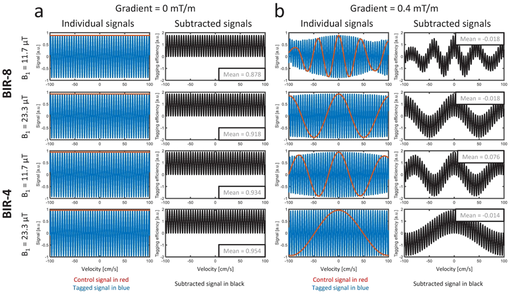
Examples from simulations of BIR-8 and BIR-4 preparations with peak B₁ of 11.7 μT and 23.3 μT, assuming a parabolic flow with 100 cm/s peak velocity, located in local gradient fields of 0 mT/m (a) and 0.4 mT/m (b). Control (red), tag (blue), and subtracted (black) signals are plotted for each. When the vessel is located in a local gradient field of 0 mT/m (a), control signal (red) is constant across all velocities. When a local gradient field is present (= 0.4 mT/m; b), perturbations are apparent in control, tag, and subtracted signals, resulting in a complex and decreased subtraction signal in parabolic flow. A more complicated pattern was observed in the complex difference signals for the longer BIR-8 preparation module with B₁ peak of 11.7 μT.

Figure 2.

Mean tagging efficiency predicted for parabolic flow as a function of the dot product of local susceptibility gradient and maximum velocity. This was calculated for a peak velocity of 100 cm/s but was similar for lower velocities. Note the efficiency falls off rapidly for faster flowing spins in the presence of local gradient. The reduced efficiency at higher products of velocity and susceptibility gradient was greater for the BIR-8 preparation and at lower peak B₁.

Simulation results for the straight tube flowing adjacent to an air-filled cylinder are shown in Figure 3. High resolution air-cavity images (Figure 3 a) at the simulated resolution (0.027 × 0.027 × 0.43 mm³) show the complex tagging behavior developed as spins move through the heterogeneous magnetic field. Signal modulation is observed in both the label and control images and is shifted downstream of the center of the field gradient. Magnitude air-cavity images (Figure 3 b) simulated using a 1-mm spatial resolution show the observed local tagging to be dependent predominantly on signal loss in the control images. Note that the simulated 1-mm resolution provides visualization for the impact of partial volume effects. Line profiles along the length of the vessel with flow from left to right of the field (Figure 3 c) as well as the tagging efficiency (Figure 3 d) are shown for both the air and a reference simulation with the air cavity replaced with water. A substantial reduction in efficiency is observed as spins pass through the field gradient, which is not observed with a homogeneous water background or when simulations are performed without particle tracking. Bloch simulations show a small post labeling delay further shifts the signal downstream (Supporting Information Figure S6).

Figure 3.

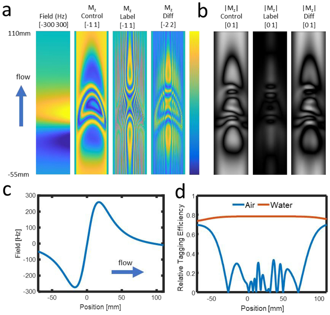
Simulated field, and Mz images along the length of the vessel (a), with brackets providing the range of lower and upper limits of the color visualization. The control image deviates substantially from the ideal uniform value of 1. When considering intravoxel signal averaging at 1 mm resolution (b) this modulation results in signal loss in the control image that results in lower signal difference despite the effective signal saturation in the label image. Taking the field values along the centerline of the vessel (c) and the resulting signal at 1 mm resolution with air and water filled wells (d), substantial signal loss is observed that is shifted downstream from the field perturbation. These results are in good agreement with those observed in physical phantoms (Figure 4).

Phantom Imaging

Simulation results were corroborated by images from phantom experiments shown in Figure 4. B₀ field maps show the local gradient surrounding the two susceptibility sources: water and air-filled wells. Note the orientation of the main B₀ field (red arrow) and direction of water flowing along a tube (blue arrow). Tag images show nearly complete signal loss in the moving water within the tube, regardless of the proximity to the susceptibility well. The control image in the presence of the matched susceptibility well (water) shows bright signal in the moving water; however, control images demonstrate signal loss in the fluid traveling past the air-filled susceptibility well with greater susceptibility resulting in a lower relative tagging efficiency. Signal loss is observed adjacent to the susceptibility well and also displaced downstream from the well. Figure 5 shows centerline plots of the gradient field (Figure 5 a), off-resonance frequency (Figure 5 b), and relative tagging efficiency at 500 (Figure 5 c) and 1000 (Figure 5 d) mL/min for both air and water-filled wells. Note the gradient is a 3D vector and the absolute value has been displayed. Signal loss is observed at the leading edge of the susceptibility induced gradient. Further, the reduced efficiency is propagated downstream, likely due to flow during both the VS-ASL preparation module but also the ~50 ms readout window used for sampling. Given the peak velocity of ~50 cm/s, during the readout, spins travel roughly 25 mm for a flow rate of 500 mL/min and 50 mm for a flow rate of 1000 mL/min.

Figure 4.

Geometry used for the physical phantom that included a susceptibility well (far left). Control, tag, and magnetic field gradient images from an agar/water gel phantom with flow at 500 mL/min, adjacent to a susceptibility insert made up of wells of either water (left) or air (right). Signal in the tube remains low for both susceptibility wells; however, the control image shows signal loss near the air susceptibility well. Correspondingly, the magnetic field gradient is much greater near the air susceptibility well whereas there is no significant gradient due to the similar susceptibility of the agar/water phantom and the water filled well.

Figure 5.

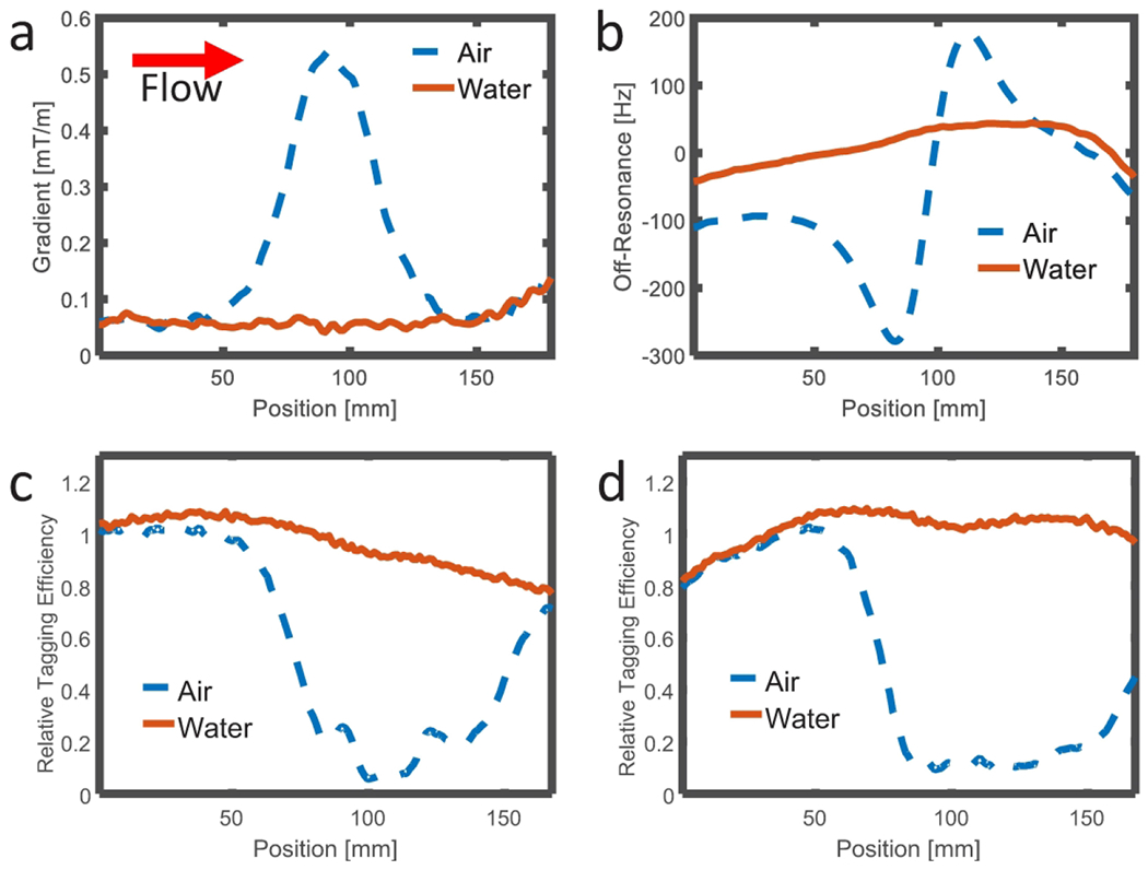
Profiles of the absolute value of the magnetic field gradient (a) and off-resonance frequency (b) measured along the centerline in the direction of flow through the tube located adjacent to the air (blue line) and water (red line) susceptibility phantoms. Corresponding profiles of the relative tagging efficiency are plotted for flow rates of 500 mL/min (c) and 1000 mL/min (d). Greater local gradient is measured along the tube adjacent to the air susceptibility well and the relative tagging efficiency is much lower in this region and immediately downstream (blue lines).

In Vivo Relative Tagging Efficiency

Sagittal and coronal limited maximum intensity projection (MIP) images of relative tagging efficiency maps are shown in Figure 6 for all subjects. Images were generated by taking a MIP of the 4D-Flow angiogram and setting the brightness based on the angiogram intensity with the color set by the relative tagging efficiency at the angiogram maximum intensity location. Relative tagging efficiency maps show relatively homogeneous efficiency in the extracranial segments of the ICAs; however, as the ICA moves intracranially, there is substantial increase in the heterogeneity of the tagging. This appears to correspond with the passage of the arteries along the bone and air-tissue interfaces, which are known to result in susceptibility induced B₀ heterogeneity. 4D-Flow angiograms ruled out the presence of stenoses or abnormal vascular anatomy. Typical source images from ASL relative efficiency mapping and the 4D-Flow complex difference from a normal healthy volunteer are shown in Figure 7. In both sagittal and axial images, vessels can be visualized that are saturated in both the control and label images while signal is observed in the reference images leading to a low relative tagging efficiency. This is most clearly visualized in the middle cerebral artery (MCA) (Figure 7, arrows) where the vessel is separated from the skull base and there is substantial surrounding brain tissue. Incidental tagging of CSF is also visualized at the base of the brain in the spinal canal and foramen magnum. These results are similar to in vivo comparisons of VS-ASL and PC-ASL, which demonstrate local signal loss in the nasal sinus as well as the ability to visualize both arterial and venous structures with the VS-ASL tagging (Supporting Information Figure S7). These MRA acquisitions did use a much longer readout (1000 ms vs. ~50 ms) to support higher resolution and SNR. Such, longer readouts are sensitive to flow transport of the signal which can spatially distort the true tagging efficiency, as seen in retrospectively subsampled images (Supporting Information Figure S8).

Figure 6.

Limited MIPs from the relative tagging efficiency maps for each volunteer including coronal (top row) and sagittal (bottom row) reformats. Similar patterns of high relative tagging efficiency are observed in the sagittal sinus, lower ICAs and BA; however, reduced relative efficiency is observed adjacent to the nasal sinus including the terminus (white arrows) and middle (yellow arrows) ICAs. Note that signal from structures including vessel segments located outside of the limited volume used for the MIP projection are not displayed.

Figure 7.

Axial and images from two different sagittal slice locations from a typical volunteer as well as limited thickness MIPs. Signal loss is visible in the middle cerebral artery (MCAs) (arrow) of the control image. The axial and sagittal difference images show high subtracted signal in the blood vessels except for in the MCAs (arrow). VS-ASL relative tagging efficiency maps show high efficiency in both the arterial and venous systems; however, the arteries over the cavernous sinus are not well tagged (arrow).

ROIs were measured across B₀, B₁ gradient dot product, |V|, |V_z|, and relative tagging efficiency maps. Median values were calculated for volumetric ROIs covering segmented vessels as described in Supporting Information Figure S3. The median of the median values measured from the ROIs for each subject as well as the standard deviation of the median values across all subjects are shown in Table 1. Box plots of the values from the segmented vessel ROIs are shown in Figure 8. High relative tagging efficiency was observed in the ICA C1, BA, Sup. S, Sag. S, and Tran. S segments. Conversely, the lowest median tagging efficiency was observed in the ICA C3, ICA C4-5, and MCA.

Table 1.

Median and standard deviations calculated from the median values measured in each ROI for each volunteer. Measurements were performed in all volunteers using the volumetric ROIs defined in Supporting Information Figure S3.

	B0 [mT]		B1 [%]		$\overrightarrow{g_s}·\overrightarrow{v}$ [mT/s]		|V| [cm/s]		|VZ| [cm/s]		Relative Tagging Efficiency [a.u.]
Segment	Median	SD	Median	SD	Median	SD	Median	SD	Median	SD	Median	SD
ICA C1	−0.0003	0.0010	96.4	3.0	0.008	0.003	17.5	3.7	15.5	3.8	0.51	0.05
ICA C3	0.0034	0.0016	104.4	10.5	0.050	0.044	22.4	5.3	19.8	4.6	0.31	0.13
ICA C4-5	0.0005	0.0014	100.7	7.3	0.043	0.009	21.1	3.9	7.3	2.1	0.12	0.07
MCA	0.0003	0.0005	99.1	2.8	0.006	0.002	24.7	5.6	4.1	1.0	0.10	0.11
BA	0.0017	0.0012	105.4	4.7	0.024	0.033	22.3	5.4	19.2	5.4	0.42	0.12
Trans. S	0.0007	0.0007	94.9	3.6	0.004	0.002	13.1	2.4	2.6	1.0	0.33	0.05
Sag. S	−0.0007	0.0004	95.0	4.1	0.003	0.000	16.0	2.2	15.1	2.0	0.39	0.04
Sup. S	0.0007	0.0011	78.6	5.9	0.003	0.001	11.0	1.5	2.6	0.6	0.30	0.07

Figure 8.

Box plots showing regional measurements for a) B0, b) B1, c) Gradient dot product, d) magnitude of velocity, e) magnitude of velocity in z-direction, and f) relative tagging efficiency. Regions were derived from segments defined in Supporting Information Figure S3.

Impact of Changes to the Local Gradient

Sagittal magnetic field gradient maps (Figure 9 a) demonstrate significant change in the local gradient field across the volunteer’s head when comparing the three external shim gradient settings in the S/I direction (0.00 mT/m, 0.08 mT/m, and 0.17 mT/m from left to right). Sagittal MIP angiograms show signal dropout in the region of rapid flow over the nasal sinus for all gradients (Figure 9 b, arrows) with greater signal loss in other fast flowing vessels with increasing local gradient. Sagittal relative tagging efficiency maps confirm decreasing efficiency in high velocity vessels with greater local gradient (Figure 9 c). Relative global decreases in single-slice mid-brain axial perfusion maps are observed with increasing gradient (Figure 9 d).

Figure 9.

Sagittal gradient field maps (a) and MIP angiograms (b) acquired with 3 external shim gradient settings in the S/I direction (0.00 mT/m, 0.08 mT/m, and 0.17 mT/m from left to right). Signal dropout is seen in the region of rapid flow over the nasal sinus for all shim gradient values (b, arrows) with greater lost in other fast flowing vessels with increasing local gradient.

Discussion

Velocity selective approaches have advantages over other tagging strategies, including insensitivity to post labeling delay selection and the ability to label complex vascular geometries; however, there are clearly challenges in achieving uniform tagging efficiency and avoiding incidental tagging of CSF or background static tissue. This work has provided a method using an accelerated acquisition with a minimum post labeling delay time combined with the VS-ASL preparation to readily visualize the spatial distribution of relative tagging efficiency. In the in vivo experiments using a BIR-8 preparation, this strategy was used to visualize reduced relative tagging efficiency in the major feeding arteries of the brain and the regional correlation of efficiency with local velocity, off-resonance, magnetic field gradient, and the local B₁ field. These experiments, as well as data in physical phantoms and numerical simulations, suggest that magnetic field heterogeneity substantially reduces velocity selective tagging efficiency for the BIR-8 preparation. Specifically, the magnetic field heterogeneity leads to signal loss in the control images.

VS-ASL relative tagging efficiency mapping provides the ability to assess performance across a range of individual morphology and physical characteristics, including variations in regional blood velocity or air-tissue interfaces. This has multiple downstream effects on the prospective use of VS-ASL as a quantitative tool for perfusion. Current perfusion quantification assumes uniform tagging efficiency across the entire tagged volume. While this limitation is understood within the scientific community, the approach we present here may allow more accurate modeling through the incorporations of regional relative tagging efficiency or through improved characterization of the tagging efficiencies impact on downstream perfusion signal. More prospectively, the methods proposed hold the potential to evaluate new strategies for robust tagging. By mapping relative tagging efficiency in realistic in vivo settings, the tagging efficiency trade-offs can be evaluated for given preparation modules. For example, the BIR-8 preparation used in this manuscript results in a high level of robustness to eddy currents. Alternative preparation modules (e.g. BIR-4) offer a theoretical reduction of sensitivity to static field gradients at the cost of higher sensitivity to eddy currents. Relative tagging efficiency mapping allows for the in vivo evaluation of these trade-offs. Further work using tagging efficiency mapping may also elicit the design of strategies which are insensitive to both eddy currents and static B₀ heterogeneity, however, it is outside of the scope of our work to make specific recommendations on the use of given preparation designs. Qin et al.²³ demonstrated the use of a similar measure of tagging efficiency for VS-ASL using pulse trains and investigated signal losses due to static B₀, T₂, and acceleration using a Cartesian acquisition. This approach provided the ability to visualize localized changes in the labeling patterns and did identify signal loss in the petrous segment of the ICA similar to this work. In our work, we found signal loss in both the label as well as control images in the presence of local susceptibility gradients and rapid blood flow. The loss was substantially higher than that of PC-ASL using the identical imaging readout, suggesting the errors were due to labeling. Further work is needed to evaluate the generalizability of these results to other preparation modules.

The currently proposed VS-ASL tagging approach does have restrictions which limit the quantitative accuracy and spatial fidelity of the mapping. A relatively long, high-resolution data acquisition is required for visualization of tagging efficiency in the small vessels as well as larger ones. Even so, it was not possible to visualize tagging in small arterial feeders (<3 mm); which are expected to contribute to the tagging efficiency. There are necessary trade-offs between spatial resolution and scan time that prevent the acquisition of substantially higher resolution. These also impact the quantification of the tagging efficiency due to partial volume effects and SNR. Further, the spatial localization is limited by bulk flow transport during the tagging module and subsequent imaging. For in vivo experiments, a BIR-8 VS-ASL preparation was used with 67 ms total prep time including crushing gradients and a 20-ms small post labeling delay. This was followed by a ~47 ms segmented readout leading to an overall measurement time of 114 ms from the start of the first RF pulse. Given an expected peak velocity of approximately 60 cm/s in the carotid artery, individual water molecules would travel 2.5 cm during the prep, 2.8 cm during the readout, and 6.9 cm overall during the measurement. Thus, the measured relative tagging efficiency is displaced downstream and represents an average over a much larger vessel segment than indicated by the spatial resolution. This spatial displacement limits the value in pixelwise correlations of the undistorted measures of velocity and magnetic fields. Beyond this, there are also limitations to absolute quantification based on T₁, as the utilized TR of 2 s also does not allow for complete T₁ recovery between tag/control interleaved pairs. Since no 90° magnetization reset pulses were applied between the interleaved tag and control sampling acquisitions, this leads to differential starting magnetization for the control, label, and reference images. The relative efficiencies we reported were not corrected for this or for decay during the imaging readout. Due to these confounders, the maximum expected efficiency would be 0.72. This is based on Bloch simulation of the pulse sequence, including the BIR-8 module, imaging module, and prescribed delays in the label, control, and reference images. This did not account for issues with flow into the brain or tagging efficiency losses from susceptibility, B₀, or B₁; and the Bloch simulations were found to overpredict the measured _{in vivo} tagging efficiency. This discrepancy is likely due to impacts of partial volume during the ROI measurements, SNR, B₀, B₁, and susceptibility induced gradients.

In this work, we utilized a radial acquisition trajectory and though it is not a requirement of the approach, there are advantages to radial acquisition in this setting. Specifically, as mentioned above, the measurement of tagging efficiency is highly impacted by the measurement time. 3D radial is readily compatible with advanced reconstructions and resilient to errors from motion, flow, and data inconsistencies. As each individual radial line samples the center of k-space, the overall contrast is averaged across the time of the segmented readout. In this work, we collected only 9 lines of k-space per preparation leading to considerable imaging acceleration factors. Even so, there is substantial spatial distortion of the tagging efficiency due to flow. Undersampled Cartesian acquisition with advanced reconstruction may be feasible although achieving sufficient image quality may be challenging. The choice of peak B₁ for this study was based on the maximum achievable B₁ for in vivo imaging including accommodating larger volunteers of up to 280 lbs when using the integrated body coil for RF excitation. RF pulses were also drive roughly 40% higher than the adiabatic threshold. Other studies (Guo et al.¹⁷) have looked at higher peak B₁ that may be possible with different imaging setups or different body coil designs. Further, recent work has proposed a preparation scheme using dynamic phase cycling for higher robustness to field heterogeneities.³⁹ Future work is needed to explore the quantification of VS-ASL tagging efficiency as well as its utilization to assess and optimize performance of developing preparation pulses.

Conclusion

We have demonstrated an approach to map the relative spatial uniformity of VS-ASL preparation pulses. We have also demonstrated the use of this technique in assessing the impact of magnetic field gradient and blood velocity on a BIR-8 preparation pulse. Overall, VS-ASL approaches have well known advantages over other techniques for imaging slow and complex filling regions, including our MRA results which suggest this method may be used to image venous structures; however, this work also shows regional decreases in the mean tagging efficiency that were found to be dependent on the peak velocity in blood vessels and local magnetic field gradients. This was shown to lead to decreased perfusion signal as well as dropout in vessels for MRA imaging and should be considered when utilizing these methods. Care should be taken when utilizing VS-ASL, and the effect of static gradients should be weighed against other artifacts when designing tagging modules.

Supplementary Material

1

Figure S1. Diagrams of BIR-8 and BIR-4 preparation modules with alternating peak B₁ used for numerical simulations. A total of four preparation modules were simulated: (a) BIR-8 at peak B₁ = 11.7 μT with preparation time of 42 ms, (b) BIR-8 at peak B₁ = 23.3 μT with preparation time of 26 ms, (c) BIR-4 at peak B₁ = 11.7 μT with preparation time of 21 ms, (d) BIR-4 at peak B₁ = 23.3 μT with preparation time of 13 ms. Adiabatic pulses were set to have 90° RF pulse widths at 4 ms and 180° RF pulse widths at 8 ms for peak B₁ = 11.7 μT and to have 90° RF pulse widths at 2 ms and 180° RF pulse widths at 4 ms for peak B₁ = 23.3 μT. VS gradients were set to have V_c at 2.35 cm/s based on peak velocity with 1 ms delays inserted after each.

Figure S2. Slices of the digital simulation mimicking the physical phantom studies. The geometry consists of a uniform water background, a long cylindrical air cavity (diameter = 50 mm), and a tube flowing through the water bath (inner diameter = 6.5 mm, outer diameter = 10.0 mm). Flow in the tube is parabolic with a maximum velocity of 60 cm/s. Subsequently, the geometric setup is used to establish a susceptibility field assuming the tube and water bath to have the same magnetic susceptibility (−9.035 ppm) and the air having a magnetic susceptibility of 0.36 ppm. With the B0 field oriented 45° with respect to the flow, the field at 3 T is estimated using a dipole kernel. Calculations were performed over a 220 mm FOV using 0.43 mm isotropic spatial resolution resulting in the below field. Fields were subsequently cropped to just include the vessel and interpolated into 0.027 x 0.027 x 0.43 mm³, with the lowest resolution along the direction of flow.

Figure S3. Segmented images derived from 4D-Flow angiograms showing the locations of volumetric ROIs used to measure local relative tagging efficiency and contributing factors. ROIs are shown in sagittal (left) and coronal (right) views.

Figure S4. Examples from simulations of BIR-8 and BIR-4 preparations with peak B₁ of 11.7 μT and 23.3 μT, assuming a parabolic flow with 100 cm/s peak velocity and acceleration at 0 m/s² and 20 m/s², located in local gradient fields of 0 mT/m (a) and 0.4 mT/m (b). Control (red), tag (blue), and subtracted (black) signals are plotted for each. When the vessel is located in a local gradient field of 0 mT/m (a), control signal (red) is constant across all velocities with and without acceleration. When a local gradient field is present (= 0.4 mT/m; b), perturbations are apparent in control, tag, and subtracted signals, resulting in a complex and decreased subtraction signal in parabolic flow without acceleration. A more complicated pattern was observed in the complex difference signals for the longer BIR-8 preparation module with B₁ peak of 11.7 μT both with and without acceleration.

Figure S5. Mean tagging efficiency predicted for pulsatile flow as a function of peak acceleration. A pulsatile flow was simulated to have peak velocity ranged from 0 to 100 cm/s with no local gradient field applied. To add physiological relevance, acceleration was assumed to be proportional to the velocity with acceleration calculated by applying a linear scaling factor (e.g. 300 s⁻¹). This aimed to mimic the expected acceleration from laminar flow, such as the flow around the curved internal carotid arteries. The peak acceleration, at the peak velocity, ranged from 0 to 300 m/s². Mean tagging efficiencies initially oscillate within a range of 0.014 then gradually converge when the pulsatile flow reaches its peak acceleration. No distinct dropout of mean tagging efficiency was observed across the range of accelerations tested for all VS tagging modules.

Figure S6. Comparisons of Bloch simulations using the BIR-8 VS-ASL preparation performed with and without a small post labeling delay of 23.5 ms. Images are shown as a longitudinal cross section of tube from −55 to 110 mm along the tube and 6.5 mm across. This includes high resolution air-cavity images (a, d) at the simulated resolution (0.027 x 0.027 x 0.43 mm³), magnitude air-cavity images (b, e) simulated using a 1 mm spatial resolution, and a line profile of the tagging efficiency (c, f) along the length of the vessel with flow from left to right, including a reference simulation with the air cavity filled with water. Including the post labeling delay results in a shift flow of the magnetization downstream which distorts the true local labeling efficiency. In this case, the center of the vessel flows downstream ~14 mm in the 23.5 ms with the displacement parabolic.

Figure S7. Sagittal MIP angiogram images from two normal volunteers using the BIR-8 preparation. VS-ASL images (left) demonstrate the opportunity for visualization of both the arterial and venous systems but with some compromise in arterial only depiction. Note signal dropout in the VS-ASL images as arterial blood flows past the cavernous sinus (yellow arrows). PC-ASL images (right) depict only the arterial system but do not show signal loss over the cavernous sinus (yellow arrows). Both acquisitions were performed using matched scan parameters including: FOV = 22 x 22 x 18 cm³, flip angle = 8°, isotropic resolution of 0.7 x 0.7 x 0.7 mm³, TE/TR = 1.1 ms / 5.5 ms, 8600 radial projection angles, 180 projections collected between preparation pulses (990 ms sampling window), time between preparations of 4 s, scan time of 6:16 (min:sec). This is roughly accelerated by 15x relative to Nyquist sampling, although the effective acceleration is lower due to multiple coils, the smaller size of the head with respect to the FOV, and the sparsity of the blood vessels. A 3 s labeling duration was used for the PC-ASL acquisition, and both acquisitions used a minimal post labeling delay (~20 ms). Please note this acquisition used a much longer sampling window after preparation than for relative tag efficiency mapping and is thus sensitive to flow during the imaging readout (see Figure S8).

Figure S8. Sagittal and coronal MIP angiogram images from an example case in which 500 ms of look-locker data was collected using the BIR-8 preparation with 3D radial sampling, and the case was reconstructed retrospectively to resolve the effect of bulk transport on the observed tagging efficiency. The acquisition was performed using: FOV = 22 x 22 x 18 cm³, flip angle = 8°, isotropic resolution of 0.7 x 0.7 x 0.7 mm³, TE/TR = 1.1 ms / 5.6 ms, 7,743 radial projection angles, 89 projections collected between preparation pulses (498 ms sampling window). Images were retrospectively binned to 5 equal time frames and reconstructed using iterative SENSE. As can be seen with the yellow arrows, sections of the ICA initially are untagged but appears to be tagged in later frames. This is due to the transport of blood along the ICA. This is also observed in the straight sinus (green arrow) where the vein is tagged and then is filled with untagged blood from the capillary bed. These errors can lead to substantial bias in the estimated efficiency in addition to bias from T1 decay of the tag/control difference.

Table S1. Gradient waveform amplitudes and timing parameters. Separation time indicates the time between the start of the first gradient pulse until the start of the next gradient pulse.

References

- 1.van Osch MJP, van der Grond J, Bakker CJG. Partial volume effects on arterial input functions: shape and amplitude distortions and their correction. J Magn Reson Imaging. 2005;22(6):704–709. doi: 10.1002/jmri.20455 [DOI] [PubMed] [Google Scholar]
- 2.Jochimsen TH, Newbould RD, Skare ST, et al. Identifying systematic errors in quantitative dynamic-susceptibility contrast perfusion imaging by high-resolution multi-echo parallel EPI. NMR in Biomedicine. 2007;20(4):429–438. doi: 10.1002/nbm.1107 [DOI] [PMC free article] [PubMed] [Google Scholar]
- 3.Alsop DC, Detre JA. Reduced transit-time sensitivity in noninvasive magnetic resonance imaging of human cerebral blood flow. J Cereb Blood Flow Metab. 1996;16(6):1236–1249. doi: 10.1097/00004647-199611000-00019 [DOI] [PubMed] [Google Scholar]
- 4.Deibler AR, Pollock JM, Kraft RA, Tan H, Burdette JH, Maldjian JA. Arterial spin-labeling in routine clinical practice, part 1: technique and artifacts. AJNR Am J Neuroradiol. 2008;29(7):1228–1234. doi: 10.3174/ajnr.A1030 [DOI] [PMC free article] [PubMed] [Google Scholar]
- 5.Zaharchuk G, Bammer R, Straka M, et al. Arterial spin-label imaging in patients with normal bolus perfusion-weighted MR imaging findings: pilot identification of the borderzone sign. Radiology. 2009;252(3):797–807. doi: 10.1148/radiol.2523082018 [DOI] [PMC free article] [PubMed] [Google Scholar]
- 6.Wong EC, Cronin M, Wu W-C, Inglis B, Frank LR, Liu TT. Velocity-selective arterial spin labeling. Magn Reson Med. 2006;55(6):1334–1341. doi: 10.1002/mrm.20906 [DOI] [PubMed] [Google Scholar]
- 7.Fan Z, Sheehan J, Bi X, Liu X, Carr J, Li D. 3D Noncontrast MR Angiography of the Distal Lower Extremities Using Flow-Sensitive Dephasing (FSD)-Prepared Balanced SSFP. Magn Reson Med. 2009;62(6):1523–1532. doi: 10.1002/mrm.22142 [DOI] [PMC free article] [PubMed] [Google Scholar]
- 8.Zhang N, Fan Z, Luo N, et al. Noncontrast MR Angiography (MRA) of Infragenual Arteries Using Flow-Sensitive Dephasing (FSD)-Prepared Steady-State Free Precession (SSFP) at 3.0T: Comparison with Contrast-Enhanced MRA. J Magn Reson Imaging. 2016;43(2):364–372. doi: 10.1002/jmri.25003 [DOI] [PMC free article] [PubMed] [Google Scholar]
- 9.Bolar DS, Gagoski B, Orbach DB, et al. Comparison of CBF Measured with Combined Velocity-Selective Arterial Spin-Labeling and Pulsed Arterial Spin-Labeling to Blood Flow Patterns Assessed by Conventional Angiography in Pediatric Moyamoya. AJNR Am J Neuroradiol. 2019;40(11):1842–1849. doi: 10.3174/ajnr.A6262 [DOI] [PMC free article] [PubMed] [Google Scholar]
- 10.Qiu D, Straka M, Zun Z, Bammer R, Moseley ME, Zaharchuk G. CBF measurements using multidelay pseudocontinuous and velocity-selective arterial spin labeling in patients with long arterial transit delays: comparison with xenon CT CBF. J Magn Reson Imaging. 2012;36(1): 110–119. doi: 10.1002/jmri.23613 [DOI] [PMC free article] [PubMed] [Google Scholar]
- 11.Schmid S, Heijtel DFR, Mutsaerts HJMM, et al. Comparison of velocity- and acceleration-selective arterial spin labeling with [15O]H2O positron emission tomography. J Cereb Blood Flow Metab. 2015;35(8):1296–1303. doi: 10.1038/jcbfm.2015.42 [DOI] [PMC free article] [PubMed] [Google Scholar]
- 12.Guo J, Wong EC. Increased SNR Efficiency in Velocity Selective Arterial Spin Labeling using Multiple Velocity Selective Saturation Modules (mm-VSASL). Magn Reson Med. 2015;74(3):694–705. doi: 10.1002/mrm.25462 [DOI] [PMC free article] [PubMed] [Google Scholar]
- 13.Qin Q, van Zijl PCM. Velocity-selective-inversion prepared arterial spin labeling. Magn Reson Med. 2016;76(4):1136–1148. doi: 10.1002/mrm.26010 [DOI] [PMC free article] [PubMed] [Google Scholar]
- 14.Liu D, Xu F, Lin DD, van Zijl PCM, Qin Q. Quantitative measurement of cerebral blood volume using velocity-selective pulse trains. Magn Reson Med. 2017;77(1):92–101. doi: 10.1002/mrm.26515 [DOI] [PMC free article] [PubMed] [Google Scholar]
- 15.Qin Q, Qu Y, Li W, et al. Cerebral blood volume mapping using Fourier-transform-based velocity-selective saturation pulse trains. Magn Reson Med. 2019;81(6):3544–3554. doi: 10.1002/mrm.27668 [DOI] [PMC free article] [PubMed] [Google Scholar]
- 16.Schmid S, Ghariq E, Teeuwisse WM, Webb A, van Osch MJP. Acceleration-selective arterial spin labeling. Magn Reson Med. 2014;71(1):191–199. doi: 10.1002/mrm.24650 [DOI] [PubMed] [Google Scholar]
- 17.Guo J, Meakin JA, Jezzard P, Wong EC. An optimized design to reduce eddy current sensitivity in velocity-selective arterial spin labeling using symmetric BIR-8 pulses. Magn Reson Med. 2015;73(3):1085–1094. doi: 10.1002/mrm.25227 [DOI] [PubMed] [Google Scholar]
- 18.Meakin JA, Jezzard P. An optimized velocity selective arterial spin labeling module with reduced eddy current sensitivity for improved perfusion quantification. Magn Reson Med. 2013;69(3):832–838. doi: 10.1002/mrm.24302 [DOI] [PubMed] [Google Scholar]
- 19.Reese TG, Heid O, Weisskoff RM, Wedeen VJ. Reduction of eddy-current-induced distortion in diffusion MRI using a twice-refocused spin echo. Magn Reson Med. 2003;49(1):177–182. doi: 10.1002/mrm.10308 [DOI] [PubMed] [Google Scholar]
- 20.Chen Z, Zhang X, Yuan C, Zhao X, van Osch MJP. Measuring the labeling efficiency of pseudocontinuous arterial spin labeling. Magn Reson Med. 2017;77(5):1841–1852. doi: 10.1002/mrm.26266 [DOI] [PubMed] [Google Scholar]
- 21.Aslan S, Xu F, Wang PL, et al. ESTIMATION OF LABELING EFFICIENCY IN PSEUDO-CONTINUOUS ARTERIAL SPIN LABELING. Magn Reson Med. 2010;63(3):765–771. doi: 10.1002/mrm.22245 [DOI] [PMC free article] [PubMed] [Google Scholar]
- 22.Zhao L, Vidorreta M, Soman S, Detre JA, Alsop DC. Improving the Robustness of Pseudo Continuous Arterial Spin Labeling to Off Resonance and Pulsatile Flow Velocity. Magn Reson Med. 2017;78(4):1342–1351. doi: 10.1002/mrm.26513 [DOI] [PMC free article] [PubMed] [Google Scholar]
- 23.Qin Q, Shin T, Schär M, Guo H, Chen H, Qiao Y. Velocity-selective magnetization-prepared non-contrast-enhanced cerebral MR angiography at 3 Tesla: Improved immunity to B0/B1 inhomogeneity. Magnetic Resonance in Medicine. 2016;75(3):1232–1241. doi: 10.1002/mrm.25764 [DOI] [PMC free article] [PubMed] [Google Scholar]
- 24.Holmes JH, Schubert T, Sanan P, Turski PA, Johnson KM. Evaluation of Velocity Selective ASL Tagging Efficiency Utilizing Accelerated 3D Angiography. In: Proceedings of the 26th Annual Meeting of ISMRM. ; 2017:Abstract 677. [Google Scholar]
- 25.Wong EC, Guo J. BIR-4 based B1 and B0 insensitive velocity selective trains. In: 18th Annual Meeting of the ISMRM. ; 2010:2853. [Google Scholar]
- 26.Wu H, Block WF, Turski PA, et al. Non-contrast Dynamic 3D Intracranial MR Angiography using Pseudo-Continuous Arterial Spin Labeling (PCASL) and Accelerated 3D Radial Acquisition. J Magn Reson Imaging. 2014;39(5):1320–1326. doi: 10.1002/jmri.24279 [DOI] [PMC free article] [PubMed] [Google Scholar]
- 27.Wu H, Block WF, Turski PA, Mistretta CA, Johnson KM. Noncontrast-enhanced three-dimensional (3D) intracranial MR angiography using pseudocontinuous arterial spin labeling and accelerated 3D radial acquisition. Magn Reson Med. 2013;69(3):708–715. doi: 10.1002/mrm.24298 [DOI] [PMC free article] [PubMed] [Google Scholar]
- 28.Nagel AM, Laun FB, Weber M-A, Matthies C, Semmler W, Schad LR. Sodium MRI using a density-adapted 3D radial acquisition technique. Magn Reson Med. 2009;62(6):1565–1573. doi: 10.1002/mrm.22157 [DOI] [PubMed] [Google Scholar]
- 29.Johnson KM, Fain SB, Schiebler ML, Nagle S. Optimized 3D Ultrashort Echo Time Pulmonary MRI. Magn Reson Med. 2013;70(5):1241–1250. doi: 10.1002/mrm.24570 [DOI] [PMC free article] [PubMed] [Google Scholar]
- 30.Pruessmann KP, Weiger M, Bornert, Peter, Boesiger P. A gridding approach for sensitivity encoding with arbitrary trajectories. In: Proceedings of the 8th Annual Meeting of ISMRM. ; 2000:Abstract 276. [Google Scholar]
- 31.Kannengiesser SAR, Brenner AR, Noll TG. Accelerated image reconstruction for sensitivity encoded imaging with arbitrary k-space trajectories. In: Proceedings of the 8th Annual Meeting of ISMRM. ; 2000:Abstract 155. [Google Scholar]
- 32.Pruessmann KP, Weiger M, Börnert P, Boesiger P. Advances in sensitivity encoding with arbitrary k-space trajectories. Magnetic Resonance in Medicine. 2001;46(4):638–651. doi: 10.1002/mrm.1241 [DOI] [PubMed] [Google Scholar]
- 33.Lustig M, Donoho D, Pauly JM. Sparse MRI: The application of compressed sensing for rapid MR imaging. Magn Reson Med. 2007;58(6):1182–1195. doi: 10.1002/mrm.21391 [DOI] [PubMed] [Google Scholar]
- 34.Johnson KM, Lum DP, Turski PA, Block WF, Mistretta CA, Wieben O. Improved 3D Phase Contrast MRI with Off-resonance Corrected Dual Echo VIPR. Magn Reson Med. 2008;60(6):1329–1336. doi: 10.1002/mrm.21763 [DOI] [PMC free article] [PubMed] [Google Scholar]
- 35.Reeder SB, Wen Z, Yu H, et al. Multicoil Dixon chemical species separation with an iterative least-squares estimation method. Magnetic Resonance in Medicine. 2004;51(1):35–45. doi: 10.1002/mrm.10675 [DOI] [PubMed] [Google Scholar]
- 36.Yu H, Shimakawa A, McKenzie CA, Brodsky E, Brittain JH, Reeder SB. Multi-Echo Water-Fat Separation and Simultaneous R2* Estimation with Multi-Frequency Fat Spectrum Modeling. Magn Reson Med. 2008;60(5):1122–1134. doi: 10.1002/mrm.21737 [DOI] [PMC free article] [PubMed] [Google Scholar]
- 37.Sacolick LI, Wiesinger F, Hancu I, Vogel MW. B1 mapping by Bloch-Siegert shift. Magn Reson Med. 2010;63(5):1315–1322. doi: 10.1002/mrm.22357 [DOI] [PMC free article] [PubMed] [Google Scholar]
- 38.Alsop DC, Detre JA, Golay X, et al. Recommended Implementation of Arterial Spin Labeled Perfusion MRI for Clinical Applications: A consensus of the ISMRM Perfusion Study Group and the European Consortium for ASL in Dementia. Magn Reson Med. 2015;73(1):102–116. doi: 10.1002/mrm.25197 [DOI] [PMC free article] [PubMed] [Google Scholar]
- 39.Liu D, Li W, Xu F, Zhu D, Shin T, Qin Q. Ensuring both velocity and spatial responses robust to field inhomogeneities for velocity-selective arterial spin labeling through dynamic phase-cycling. Magnetic Resonance in Medicine. n/a(n/a). doi: 10.1002/mrm.28622 [DOI] [PMC free article] [PubMed] [Google Scholar]
Associated Data
This section collects any data citations, data availability statements, or supplementary materials included in this article.
Supplementary Materials